2. Critical Analysis of the Present Knowledge
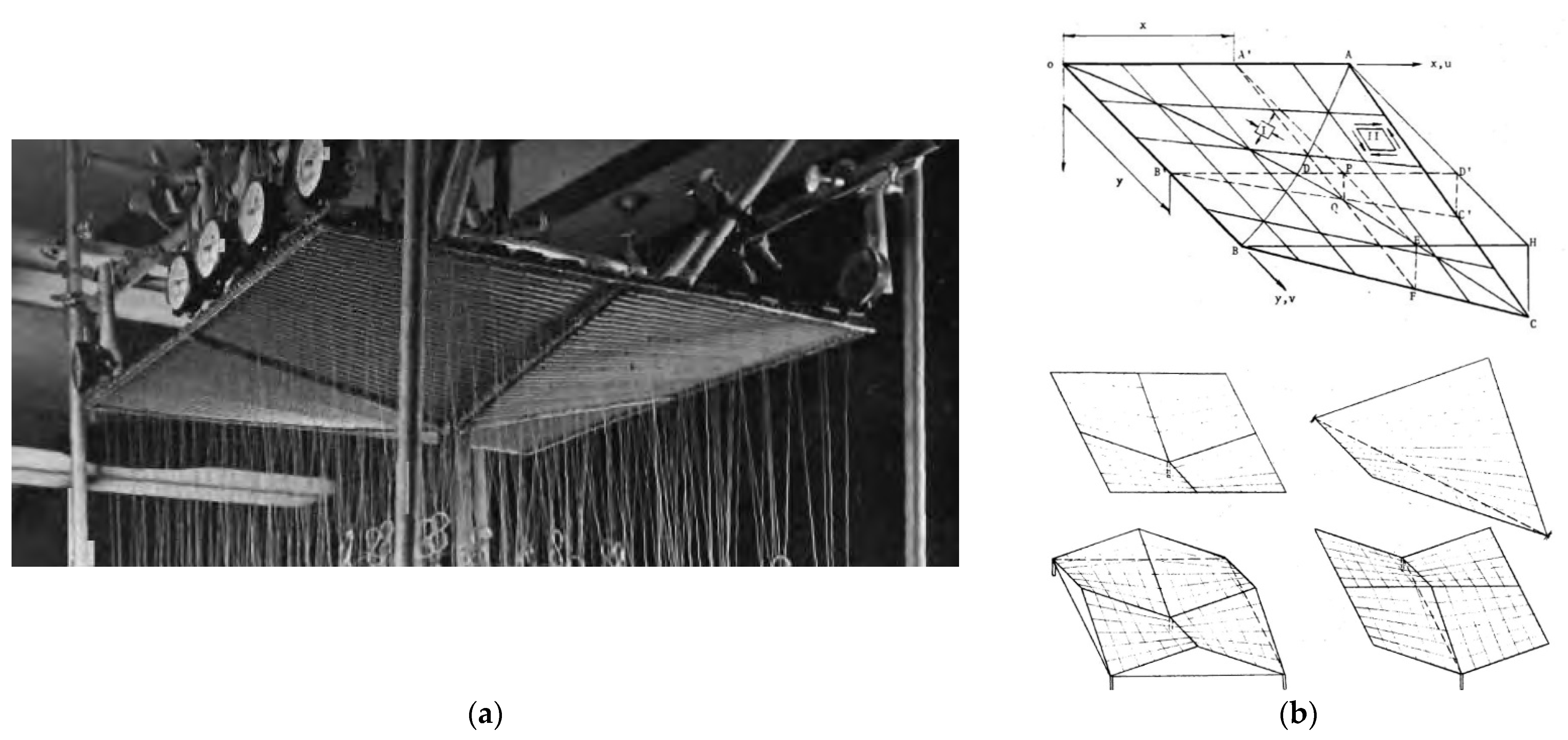
The research into the shape transformations of the nominally flat thin-walled corrugated steel sheets was initiated by Nilson in the 1970s. In the initial phase, the studies concerned the geometric and mechanical properties of complete shells transformed into the forms of central hyperbolic paraboloid sectors [
8]. In order to increase the stiffness and critical loads of the transformed folded shells, two layers of folded sheets arranged in two orthogonal directions were used by the Winter team [
9]. There were only created shallow double-layer shells characterized by a small transformation degree.
The degree can easily be increased by using single-layer sheeting at the expense of reducing the transverse stiffness of the transformed coating. Gioncu and Petcu developed a computer program for the calculation of the critical loads of the transformed shells [
10]. The results of these tests point at the fact that the transformed single corrugated shells can be regarded as working in a membrane state.
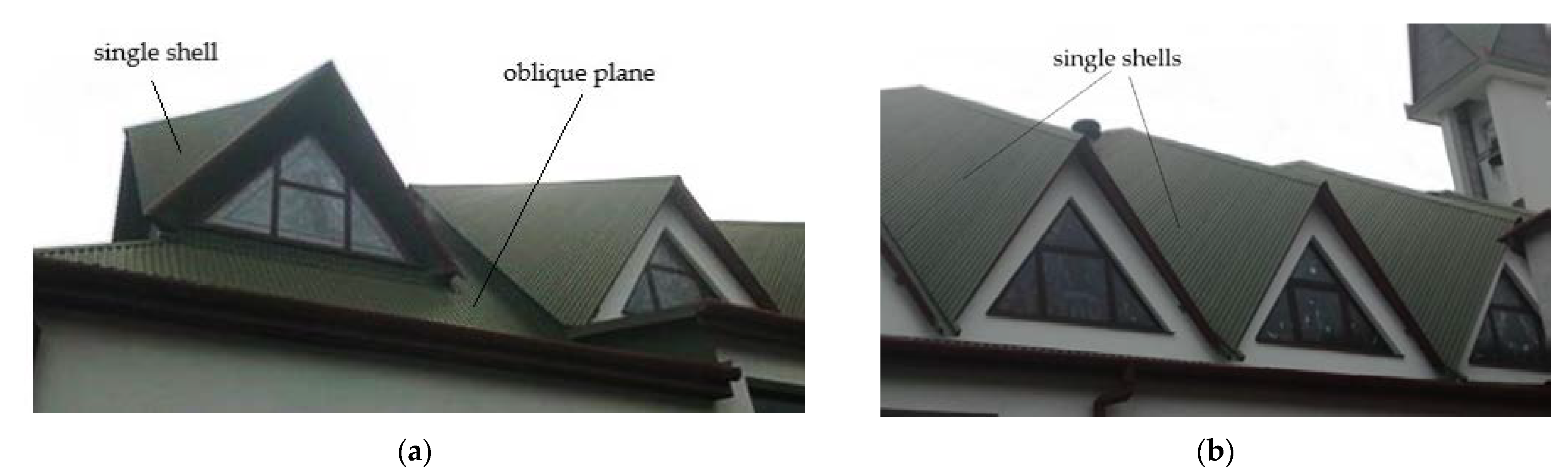
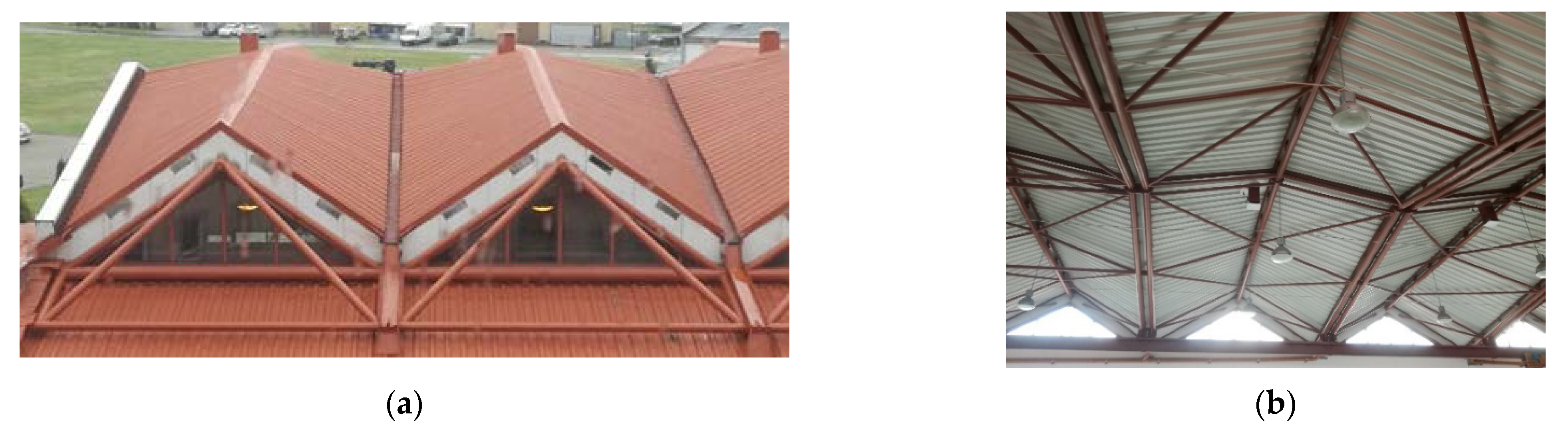
The diversity, ridge, stiffness, and critical load of the transformed folds can significantly be increased by assembling several single shell units into one continuous ribbed shell roof structure (
Figure 4a). The team led by Winter conducted comprehensive studies and published consistent results on the static-strength work of several single shells and shell structures composed of four quarters of the hyperbolic paraboloid central sectors arranged in different configurations (
Figure 4b). Parker published the supplementary research results concerning the static-strength work of the complete coatings and [
11].
The team led by Gergely presented a uniform description of the static-strength work of the single and complex transformed shells based on a relatively wide range of tests [
12]. Simultaneously with the Gergely’s team, similar tests and analysis were conducted by Fisher et al. [
13] in the field of static work and critical loads of the complete and complex hyperbolic paraboloid shells. The results of the tests and analysis of the work of the folded coatings were collected by Davis and Bryan to indicate the effective methods for shaping the shells [
14].
The abovementioned researchers indicated the great theoretical possibilities of shaping various ruled forms made up of the transformed folded sheets with an open profile. Ultimately, on the basis of the tests and analysis carried out, they found that the encountered significant material and technological limitations drastically reduce the possibility of shaping the diversified shell forms of transformed sheeting to one basic type of the shallow hyperbolic paraboloids called hypars [
12].
Therefore, it is reasonable to shape the ribbed structures composed of many single transformed shells by means of complex systems of complete ruled shells separated by sets of planes containing common or mutual displaced sections of the edge lines of these shells. Biswas and Iffland proposed a concept of such a system composed of many congruent transformed single shell units distributed over a sphere by means of a bundle of planes [
15]. The transformed folded shells made up of aluminum or PVC “Selchim” corrugated plastic sheets were analyzed by Samyn [
16]. The complete shells are shaped as revolved hyperboloids or right hyperbolic paraboloids limited by spatial quadrangles. Pottman proposed a comprehensive method of shaping the systems of planes separating subsequent smooth shell sectors in an arbitrary surface [
17].
Reichhart developed a novel method for shaping the complete transformed thin-walled corrugated shells to increase their diversity, ridge, and transformation degree [
18]. In accordance with Reichhart’s algorithm, the nominally flat single-layer sheeting is transformed into the position of the rigidly fixed directrices so that a freedom of the transverse width and height changes of all shell folds is assured. The previously mentioned methods did not provide such a freedom. Therefore, the effort of the transformed sheeting designed by means of these methods is significantly higher, and its critical load and ridge are significantly smaller compared to the shells formed by means of Reichhart’s method. Reichhart’s analysis carried out on the basis of the results of the tests allowed him to develop a method for calculating the shape, length, and mutual position of each shell directrix. The designed sheets do not have to be loaded with additional transverse forces to adjust their longitudinal edges or neutral axes to the positions of the selected rulings of an arbitrary ruled surface modeling the transformed roof shell.
On the basis of the results of the performed tests, Abramczyk noticed a significant role played by the contraction of each transformed shell sheeting in creating the effectively transformed thin-walled folded shells [
1]. Abramczyk extended the Reichhart method and included the condition related to the central location of the contraction in the effectively transformed folded shells.
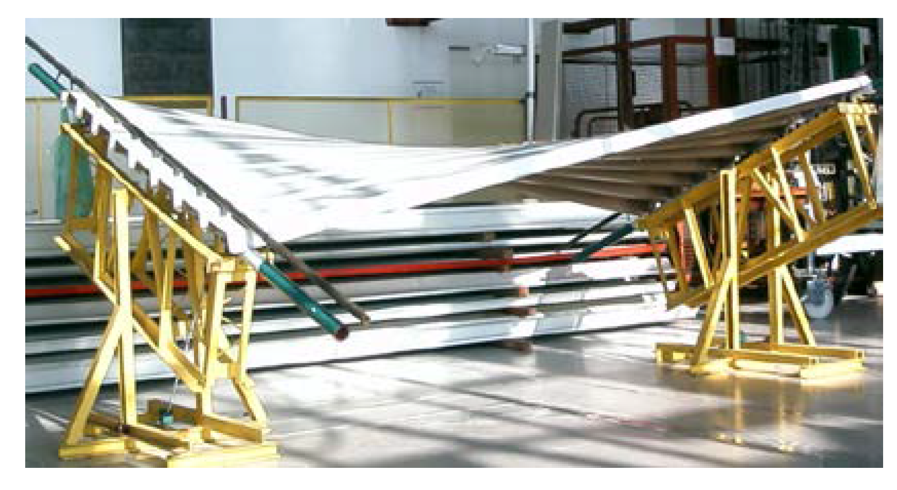
Reichhart also developed a simple method of composing of a large number of identical complete transformed shells into a ribbed structure arranged on an oblique plane (
Figure 2 and
Figure 5) [
19]. Abramczyk developed a much more complex method for regular arrangement of many complete shell units in the three-dimensional Euclidean space (
Figure 6) based on the so-called reference surface [
3]. The method results from the experimental studies and computer simulations of the transformed complete thin-walled folded shells [
20]. It is possible to combine different shell units into one regular structure whose general form is similar to the arbitrary regular surface with almost free curvature using in constructions [
21,
22].
The properties of several thin-walled structures were detailed by Wei-Wen [
23]. They can be used in shaping of the elastically transformed roof shells. Marin et al. [
24] extended the classical theory of elasticity developed by Green and Lindsay in terms of the theory of thermo-elasticity for dipolar bodies. A novel method for a solution to a dynamical mixed problem was presented using a reciprocal theorem and not very restrictive conditions [
25].
It is significant to investigate the space around the designed free-form building, its physical form and cultural patterns appearing in a whole spatial system. The relation between the formation of the urban space and the social experience of the human self was considered by Sharma [
26]. The design syntax of urban greenways should also be taken into account. The mathematics-based graph studies of patterns and shapes, thermal based photography, and morphology to perform imagery-derived deductions on the design syntax were carried out by Hasgül [
27].
Morphological shaping of buildings using many features specific to architectural, industrial, and structural design must be accomplished. Morphology is the study of the forms taking into account the relationships occurring between the function, structure, internal and external texture, static-strength work, and comfort conditions. Systematic morphology was defined by Eekhout as “the study of the system, rules and principles of form [that] has led to the interpretation of the study of the geometry of regular three-dimensional bodies or forms, usually known as polyhedra” and it plays a significant role in the design process [
28]. The analogous universal systems of planes called polyhedral reference networks are utilized in this article.
4. The Method’s Concept
The following concept of the research was adopted. The previously developed method was significantly extended and includes activities and objects that allow one to search for special rules relating to diversification of the visual patterns combined with many complete shells to achieve unconventional regular roof structures. The formulas governing the patterns result from the method of defining and arranging the single shell units in the three-dimensional space in an orderly and regular manner. For example, a reference surface and a set of division coefficients defining the location of the characteristic vertices of the designed structure can be utilized. The search for the relationships begins with the observation and description of the properties of the continuous ribbed shell roof structures.
For this purpose, a
z-symmetric roof structure
Ω consisting of two symmetrical and two antisymmetric parts is sought. The search starts with the determination of one symmetrical quarter of
Γ. At the beginning, a single central shell
Ω11 is created by means of a central tetrahedral mesh
Γ11 and a central quadrilateral mesh
Bv11 (
Figure 8). The subsequent meshes
Γij,
Bvij and
Ωij of the nets
Γ,
Bv and
Γ are symmetrically arranged with respect to the
z-axis-symmetric
Ω11 in the orthogonal and diagonal directions.
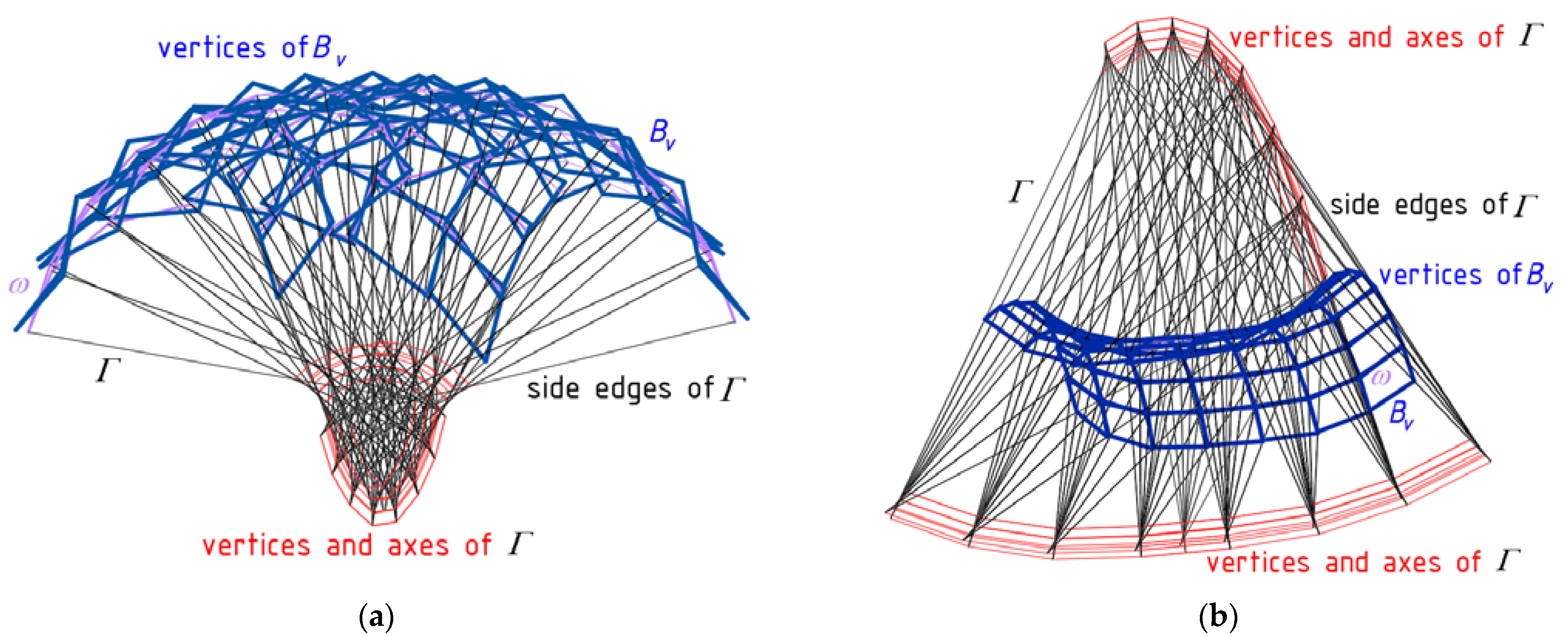
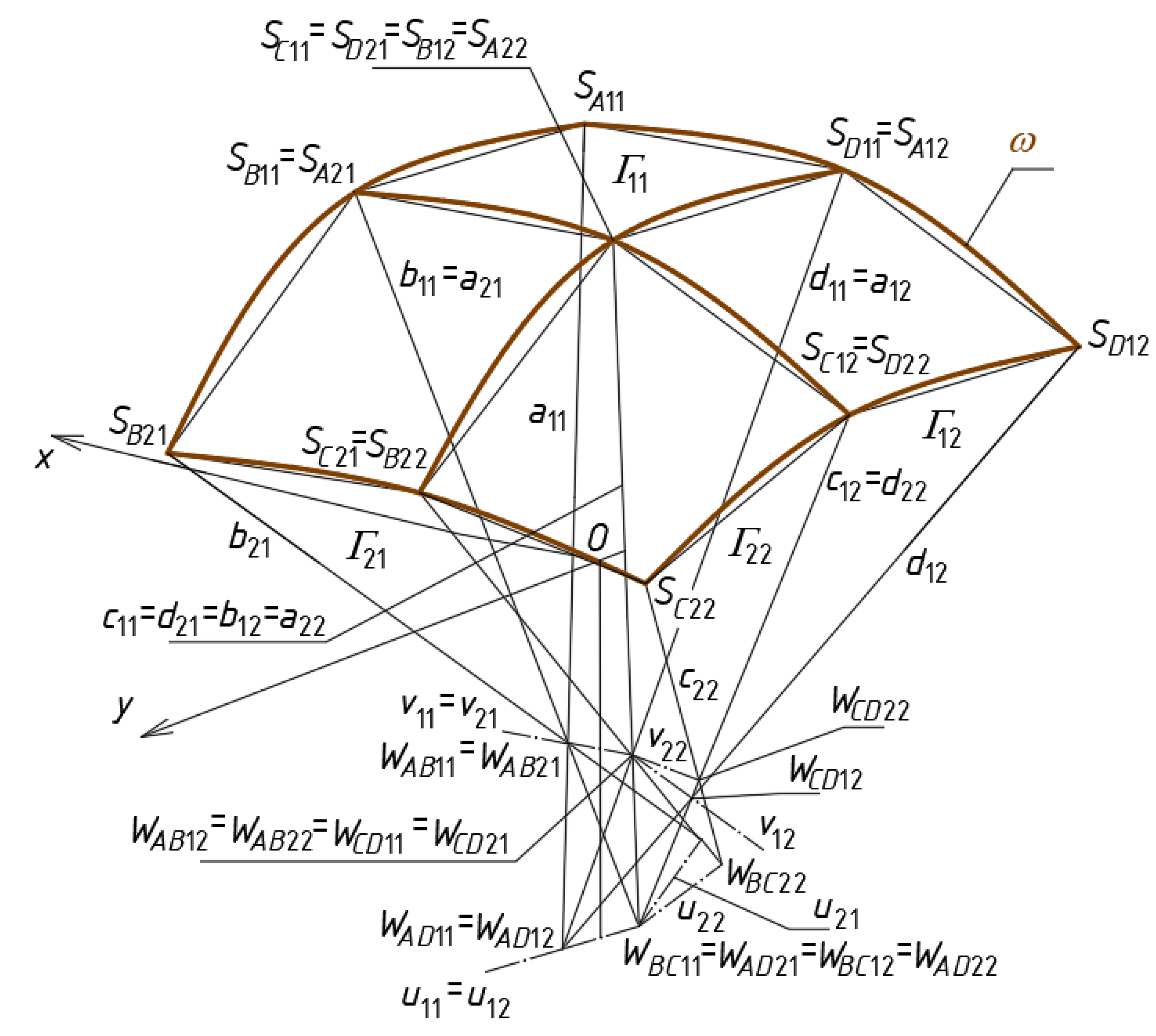
The characteristic feature of the reference network
Γ is that each single mesh
Γij is a specific tetrahedron with four vertices
WABij,
WCDij,
WADij and
WBCij, two axes
uij and
vij, four side edges
aij,
bij,
cij and
dij, four triangular side walls (
WABijWCDijWBCij), (
WABijWCDijWADCij), (
WBCijWADijWABij) and (
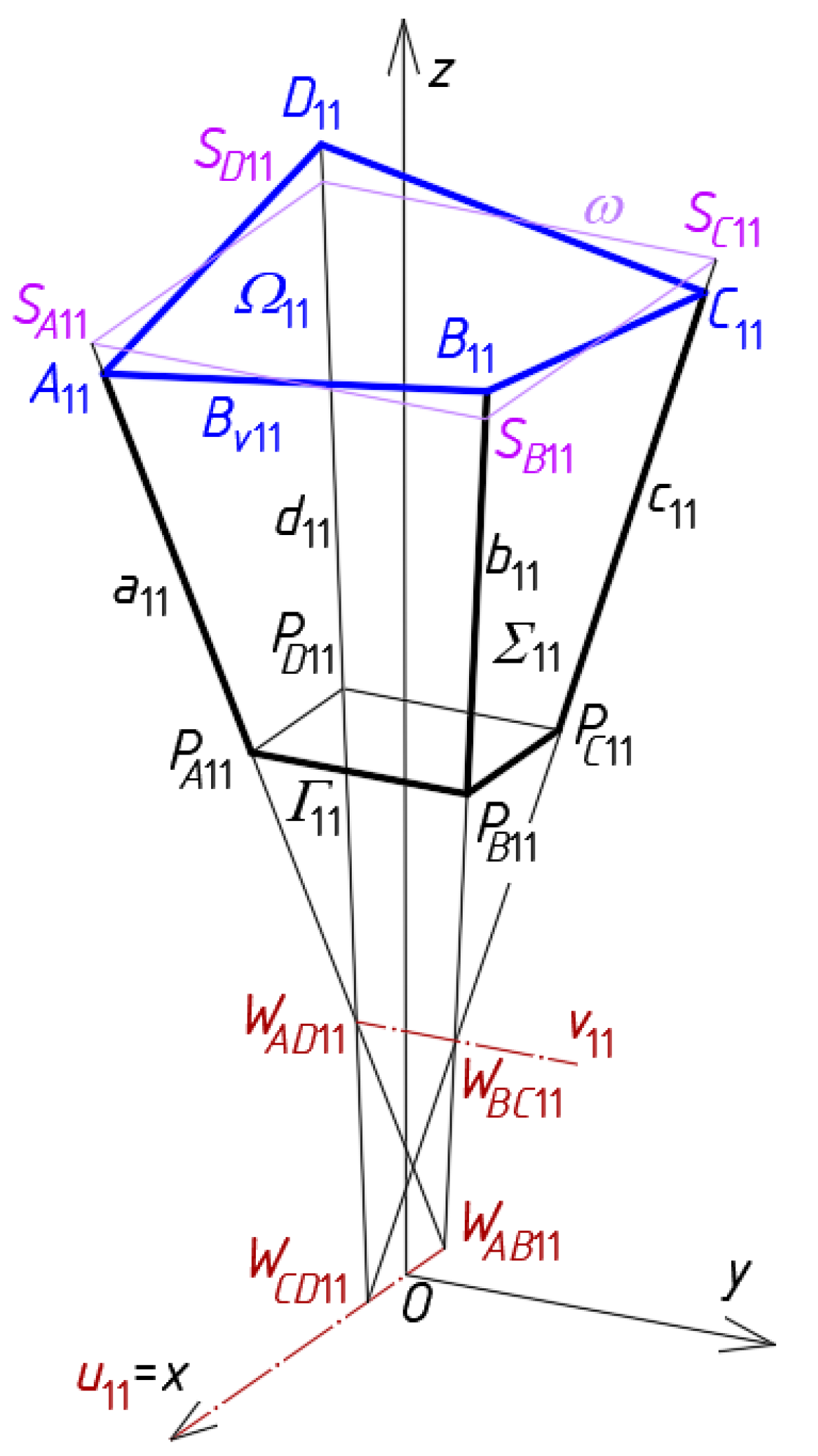
WBCijWADijWCDij) contained in four planes defined by the above vertices. For the first mesh
i =
j = 1 (
Figure 8).
In order to obtain the tetrahedron
Γ11, the coordinates of its four vertices
WAB11,
WCD11,
WAD11 and
WBC11 must be defined based on a global coordinate system [
x,y,z] [
3,
21]. The positions of the points
SA11,
SB11,
SC11 and
SD11 are defined with the following division coefficients d
SA11 = (
WAB11,
WAD11)\
SA11, d
SB11 = (
WAB11,
WBC11)\
SB11, d
SC11 = (
WCD11,
WBC11)\
SC11 and d
SD11 = (
WCD11,
WAD11)\
SD11 of the pairs (
WAB11,
WAD11), (
WAB11,
WBC11), (
WCD11,
WBC11) and (
WCD11,
WAD11), where
and
is the vector starting with
WAB11 and ending at
WAD11,
m(
) is the measure of
,
is a vector with the starting point at
WAB11 and the ending point at
SA11, etc. The points
SA11, SB11,
SC11 and
SD11 together with the analogous points assigned to the other meshes of
Γ define the respective reference surface
ω.
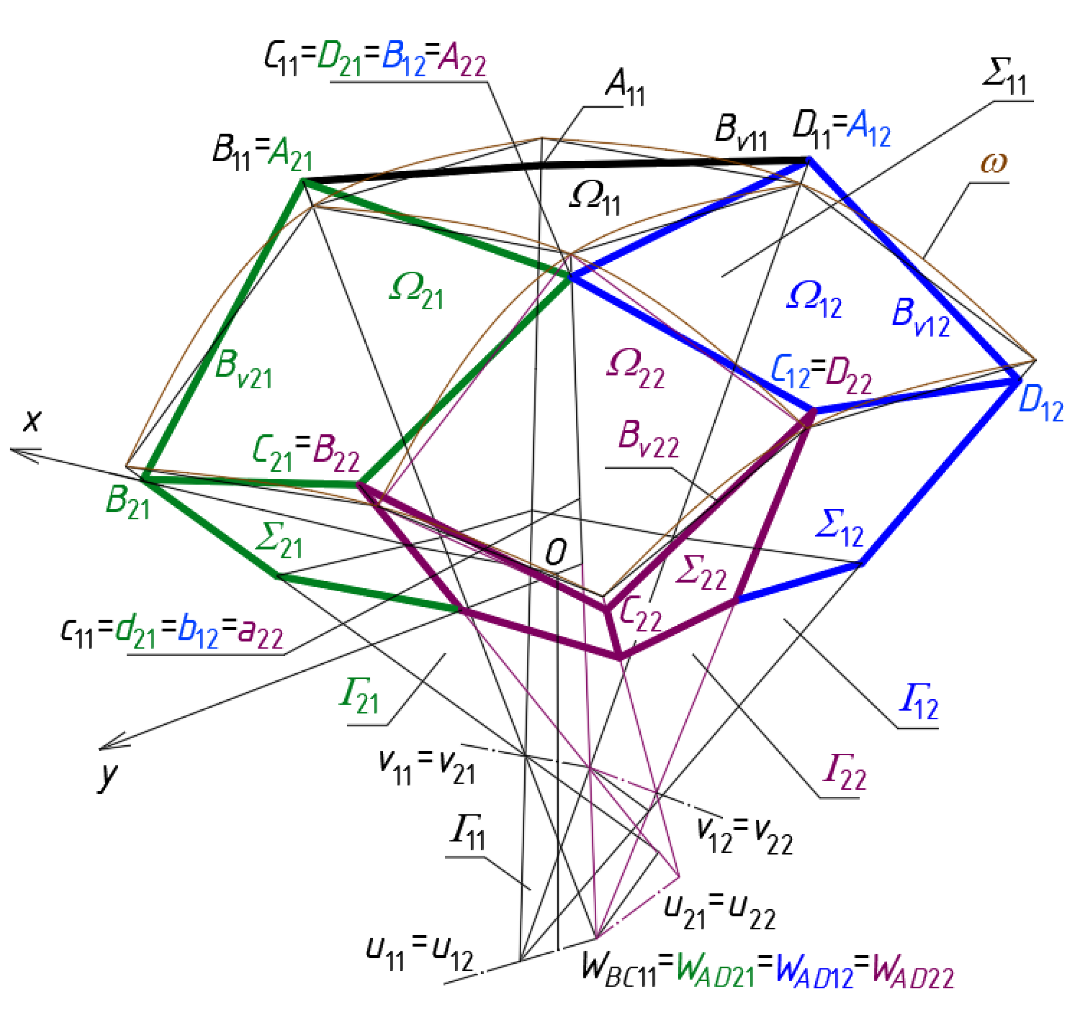
The locations of the vertices
A11,
B11,
C11 and
D11 of
Bv11 (
Figure 8) are defined by means of the vertices of
Γ11 and the following proportions:
where
is the vector with the starting point at
WAB11 and the ending point at
A11, etc. The points
A11,
B11,
C11 and
D11 determine the spatial quadrangle
Bv11 constituting the eaves of a single smooth shell segment
Ω11 modeling a single shell of a complex roof structure.
The process of shaping of the reference network Γ consists in creating subsequent tetrahedrons characterized by common planes intersecting each other in axes and side edges. To define the networks Γ and Bv, a set of the respective independent variables must be adopted and specific values have to be assigned to these variables. For all dependent variables, appropriate functions must be defined to determine the vertices of Γ and Bv.
In order to obtain the tetrahedron
Γ12 its four vertices
WAB12,
WCD12,
WAD12 and
WBC12 must be defined [
3,
29]. The vertex
WAB12 =
WCD12. Two next vertices can be calculated by means of two division coefficients as follows
where
m(
) is the measure of the vector
with the starting point at
WCD11 and the ending point at
WBC12, and
m(
) is the measure of the vector
, etc.
The vertices of the other meshes
Bvij of
Bv should be defined in the same way as
Bv11 using formulas analogous to Equations (1)–(3). Each pair of two adjacent meshes
Γij and
Γij+1 or
Γij and
Γi+1j have one common side edge contained in a plane of
Γ, for example,
Γ11 and
Γ21 has two common side edges
b11 =
a21 and
c11 =
d21, and three common vertices
WBC11 =
WAD21,
WCD11 =
WCD21 and
WAB11 =
WAB22 (
Figure 9). Four adjacent meshes
Γij,
Γij+1,
Γi+1j and
Γi+1j+1 have one common side edge
ai+1j+1 =
bi+1j =
cij =
dij+1 of
Γ, for example,
a22 =
b12 =
c11 =
d21 for
i =
j = 1.
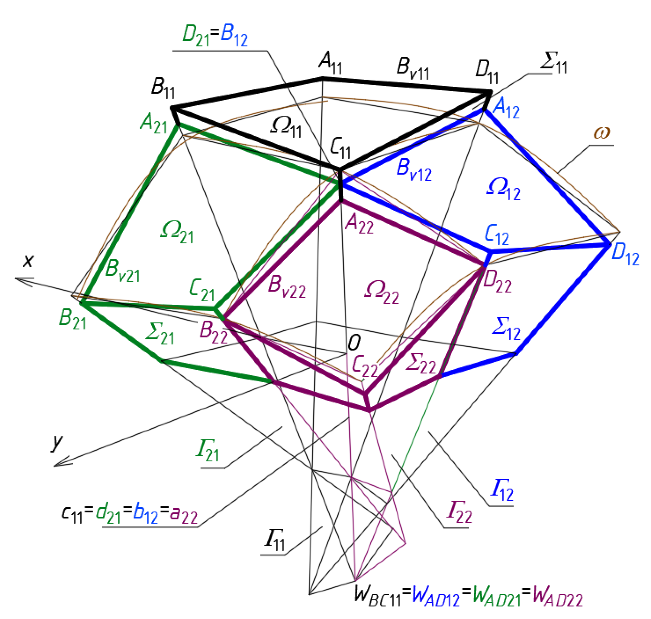
The subsequent quadrilateral meshes
Bvij of the targeted networks
Bv modeling the eaves of the examined shell roof structures are constructed based on the side edges of the auxiliary network
Γ. Following to the method’s algorithm, the subsequent adjacent quadrilateral meshes of
Bv must have common vertices
Aij,
Bij,
Cij or
Dij determined on the edges
aij,
bij,
cij and
dij (
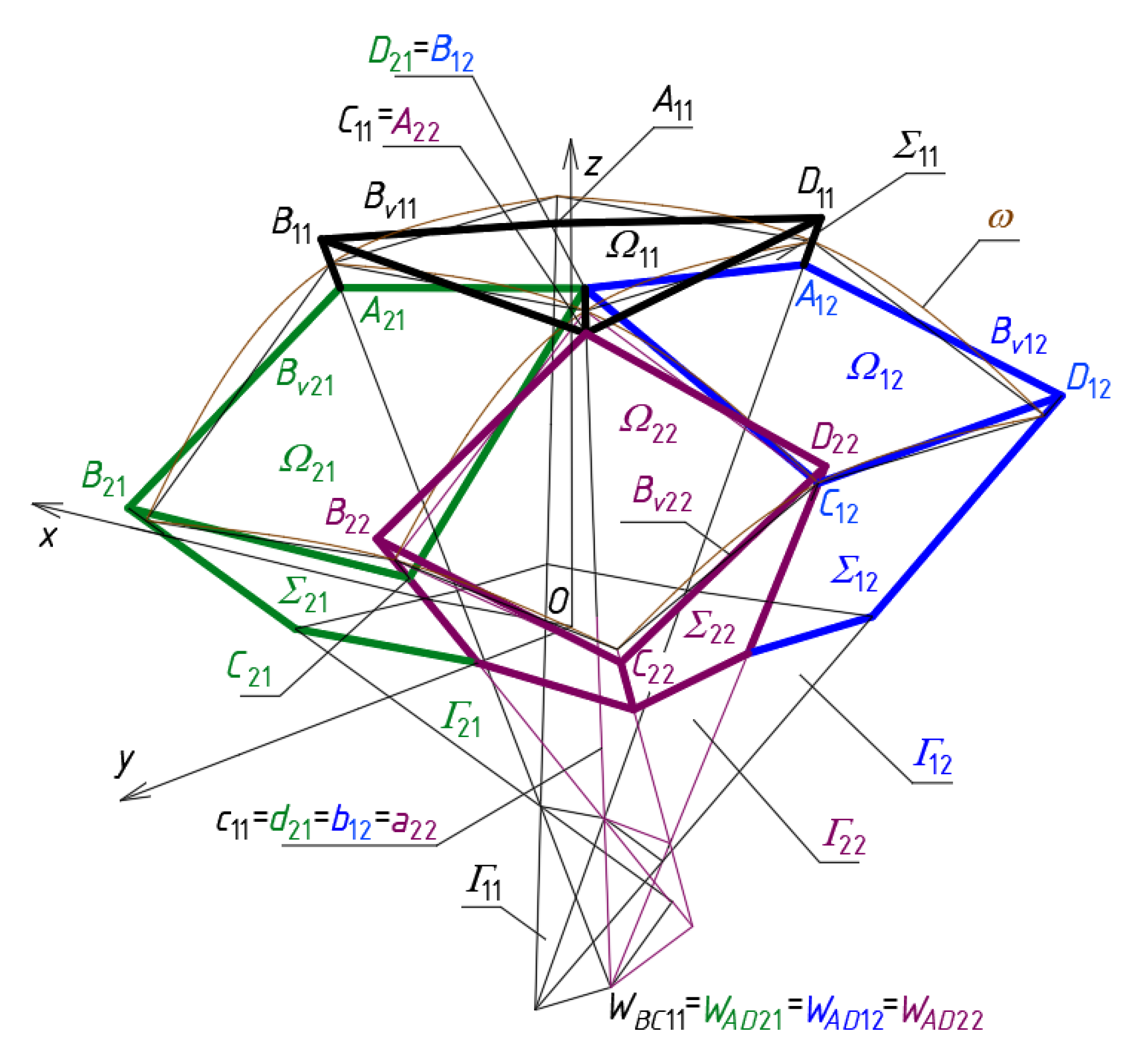
Figure 9). The specific sum of all individual shells
Ωij, determined by means of
Aij,
Bij,
Cij and
Dij, constitutes a continuous ribbed roof structure
Ω (
Figure 10). Finally, a free-form Σ of many Σ
ij is the simplified model of an entire complex building.
The complete tetrahedrons Γij can be regarded as an universal material for creating the spatial polyhedral networks modeling free-form building systems. Similarly, the single spatial quadrilateral meshes Bvij can be accepted as a material for shaping the eaves systems Bv of complex free-form roofs. In addition, the complete shell sectors Ωij are used as a universal material for creating the free-form shell roof structures Ω. After all, the abovementioned systems create three subsequent layers producing one complex material used for shaping unconventional building free forms roofed with complex shell structures.
The article primarily presents the results of the research on the geometric properties of the eaves layer Bv determining the form of the shell layer Ω. The observed properties are described with the help of the developed mathematical rules governing the systems of different patterns of the complete meshes Bvij and sectors Ωij arranged on ω. The results of these studies can be used in the design of several diversified unconventional free forms of buildings roofed with attractive and rational systems of many regular roof shells made up of transformed corrugated sheets.
In order to carry out the research, the following algorithm was developed. It forbids two adjacent meshes of
Bv or segments of
Ω to have common vertices and sides. Thus, a discontinuous net
Bv and a discontinuous structure
Ω can be created as a result of a rotation of each pair of the respective eaves segments belonging to two adjacent shell units
Ωij and
Ωi+1j or
Ωij+1 (
Figure 11). Four straight segments of each spatial quadrangle
Bvij are displaced in the respective planes of the network
Γ. Thus, the basic continuous configuration CB and the modified discontinuous configuration CP1 of the structure
Ω use the same network
Γ.
However, such a separation of the positions of the vertices belonging to the selected pairs of two adjacent meshes of Bv (Ω) requires appropriate changes in the values of the division coefficients assigned to the respective vertices of Γ of each Bvij. The goal of the research is therefore to develop a method of modifying the values of the coefficients so that different groups of discontinuous shell roof structures can be achieved. This activity requires defining some uniform conditions and adopting mathematical formulas describing the modified net Bv and structure Ω.
The designed discontinuous nets
Bv and structures
Ω can also be created as a result of translations of two respective eaves segments belonging to two adjacent shell units
Ωij and
Ωi+1j or
Ωij+1 (
Figure 12). Four straight segments of each quadrangle
Bvij can be displaced in the respective planes of
Γ.
Finally, the following algorithm based on four general steps should be adopted. The main characteristic of the algorithm is the usage of the division coefficients of the vertices of the reference polyhedral network
Γ by the vertices of a reference polygonal network
Bv (
Figure 7) and the selected points of a reference surface
ω. At the first step of the algorithm, the division coefficients are used to obtain the reference polyhedral network
Γ and the repeatability of its tetrahedral meshes
Γij, especially in the orthogonal directions. At the second step of the algorithm, the division coefficients are used to determine several points defining the reference surface
ω. The expected curvature and general form of the shell roof structure are designated in an easy and intuitive way by means of the relations defined by means of the arbitrary division coefficients.
The division coefficients are also used at the third step of the method’s algorithm to determine the vertices of the reference polygonal network
Bv. The vertices are located on the side edges of the polyhedral reference network
Γ and defined with respect to the reference surface
ω. The obtained vertices define the polygonal network
Bv composed of quadrilateral spatial meshes
Bvij. Four segments of
Bvij determine one complete shell unit
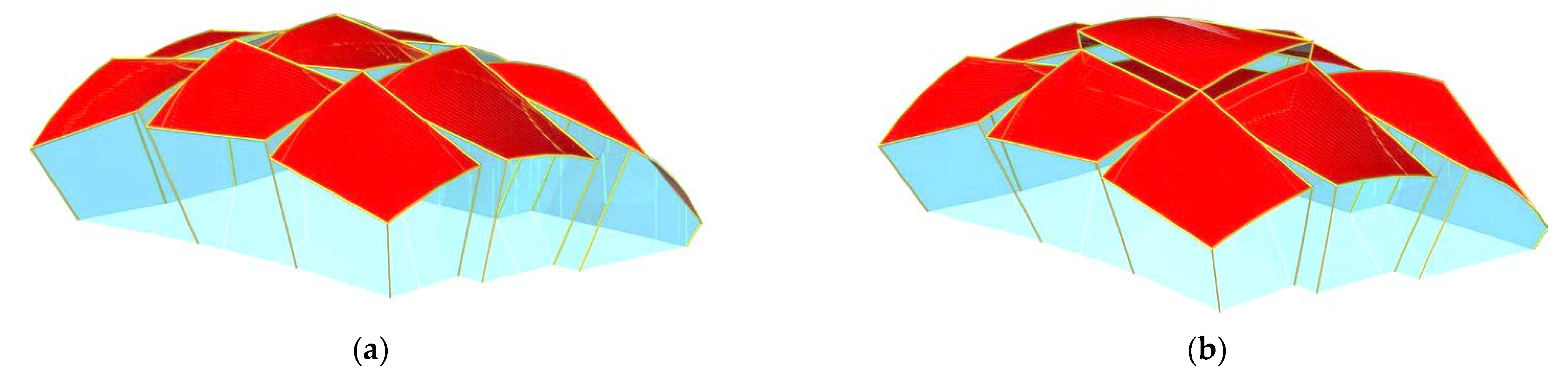
Ωij and constitute its eaves line. At this step, a basic configuration CB of the sought-after shell roof structure
Ω is created. The configuration is composed of many individual shells
Ωij so that the roof structure
Ω is continuous (
Figure 4b,
Figure 5a,b and
Figure 10). Each pair of two adjacent complete shells of the structure shares one edge.
The network Γ and the network Bv determine the curvature and folding of the roof structure Ω. The curvature of Ω can be determined using the properties of ω. The folding of Ω results from the ribs existing between the adjacent complete smooth shell units Ωij.
The fourth step of the method’s algorithm allows one to create several derivative configurations of the examined continuous roof structure. The derivative configurations are most often characterized by a mutual translation or rotation of the edge lines of the adjacent shells (
Figure 6a,b,
Figure 11 and
Figure 12) in the planes of
Γ. The discussion of the activities and their effects provided for in this step of the algorithm is the essential part of the research presented in this article.
The accuracy of the algorithm is comparable with the accuracy of the adopted data, and it is equal to 1 mm. This results from the 0.5 mm accuracy of the performed experimental tests and the 1 mm accuracy of the calculations of the ruling’s position of each complete shell Ωij of Ω.
5. Results
The search for the rules governing the systems of the diversified patterns of the complete transformed shells on the roof structures is presented in three examples of networks
Bv using the investigated algorithm. At the first step of the algorithm, the axes
uij and
vij, side edges
aij,
bij,
cij and
dij, and the entire
Γ are determined on the basis of the adopted vertices
WABij,
WCDij,
WADij and
WBCij [
3,
21]. This step is divided into two sub-steps requiring the designer to create: (1) the mesh
Γ11, meshes
Γi1 and
Γ1j (for
i > 1 and
j > 1) located orthogonally in relation to
Γ11, (2) meshes
Γij located diagonally relative to
Γ11,
Γi1 or
Γ1j. The sub-steps differ from each other in terms of the initial data and the actions necessary to build the subsequent single meshes
Γij. The values of the coordinates of the vertices belonging to the
Γ1s (
Figure 13a) are presented in
Table A1 in
Appendix A.
At the second step of the algorithm, all points defining a reference surface
ω are determined. In this way, the size of
Γ and the curvature of
ω are defined. For this purpose, the values of the selected division coefficients are adopted and the coordinates of the points
SAij,
SBij,
SCij and
SDij defining the reference surface
ω are calculated using Equation (1) and the initial data are published in
Table A2 in
Appendix A. The coordinates of these points are published in
Table A3 in
Appendix A.
At the third step, vertices of all quadrilateral meshes of the designed
Bv for the basic configuration CB are defined on the side edges of
Γ relative to
ω (
Figure 13b). At this step, the complete shell segments
Ωij of an entire roof structure
Ω constituting the basic configuration CB are defined on the basis of
Bvij. The adopted values of the division coefficients d
Aij, d
Bij, d
Cij and d
Dij used for achieving the
Bv vertices are presented in
Table A4 in
Appendix A. The coordinates of the
Bv and
Ω vertices calculated with the help of Equation (2) are presented in
Table A5 in
Appendix A.
The values of four division coefficients d
SijAij = (
WABij,
WADij)\(
SAij,
Aij), d
SijBij = (
WABij,
WBCij)\(
SBij,
Bij), d
SijCij = (
WCDij,
WBCij)\(
SCij,
Cij) and d
SijDij = (
WCDij,
WADij)\(
SDij,
Dij) are calculated to estimate the folding of
Ω (
Bv) related to the diversification of the locations of the vertices of
Bv relative to
ω. The coefficients are used with the positive or negative sign depending on whether the points
Aij,
Bij,
Cij and
Dij lie above or below
ω defined by means of the respective quadrangle
SAijSBijSCijSDij. The calculated coordinates of the vertices
Aij,
Bij,
Cij and
Dij are presented in
Table A6 in
Appendix A.
The ratios d
S11A11 = (
WAB11,
WAD11)\(
SA11,
A11), d
S11B11 = (
WAB11,
WBC11)\(
SB11,
B11), d
S11C11 = (
WCD11,
WBC11)\(
SC11,
C11) and d
S11D11 = (
WCD11,
WAD11)\(
SD11,
D11) are defined for
Bv11 as follows:
The above division coefficients allow one to observe the absolute differences in the mutual positions of the points
A11,
B11,
C11 and
D11 (
Figure 13c). The obtained values can easily be converted into the distances of these points from
ω. The coordinates of the
Bv vertices calculated with the help of the equations analogous to Equation (4) are presented in
Table A5 in
Appendix A.
The coefficients dSijAij, dSijBij, dSijCij and dSijDij do not give the precise information about the folding of the network Bv (structure Ω) because they express the proportions in relation to the distance of two adjacent vertices of Γ. Therefore, the proportions signifying the position of the points Aij, Bij, Cij and Dij in relation to the position of the points SAij, SBij, SCij, SDij and the position of the vertices of Γ must be preferred to present the folding more precisely.
Thus, the following double division coefficients play an important role in describing the geometrical properties of the roof structures:
If the values calculated by means of Equation (5) are greater than one, then the respective points lie above the surface ω. If the values are less than one, then the points lie below ω.
The following double division coefficients are a much more convenient and intuitive variable describing the folding of a shell roof structure:
The new division coefficients show the relative proportions of the folding of
Bv (
Ω) in relation to the positions of
ω and the respective vertices of
Γ. The values of these coefficients were calculated by means of Equation (6) for the selected meshes of
Bv. They are presented in
Table A7 in
Appendix A.
The polyhedral reference networks Γ, reference surfaces ω, polygonal networks Bv and shell roof structures Ω are the main geometric objects created by means of the investigated method in the process for shaping building free forms roofed with complex transformed corrugated shell structures. The network Bv is the most important because the edge lines of all its complete meshes Bvij determine all individual shell segments Ωij of the resultant roof structure Ω. The Bv sides are the eaves of Ωij. To create a network Bv characterized by the expected properties, the method introduces the auxiliary reference polyhedral network Γ assisting and facilitating the determination of the positions of the vertices Aij, Bij, Cij and Dij of Bv.
The main property of each reference network
Γ is that each pair of its adjacent side edges must intersect. The intersecting points of the respective pairs of two adjacent side edges denoted as
aij,
bij,
cij or
dij (
Figure 8 and
Figure 9) are called vertices
WABij,
WCDij,
WBCij and
WADij of
Γ. The edges define all planes of
Γ. It is very important that two adjacent meshes of
Bv have one common segment of their edge lines (for continuous structures
Ω) or two different segments (for discontinuous structures
Ω) contained in the same plane of
Γ, so the segments are coplanar. This property significantly simplifies the processes for shaping of the regular basic continuous configurations of
Ω and their derivative configurations.
The research on searching for the rules governing the locations of the
Bv vertices and the patterns of the complete
Ωij shells starts with the analysis of the properties of the basic configuration CB of the shell structures shown in
Figure 10 and
Figure 13. The configuration CB allows one to create a so-called continuous roof structure
Ω. This configuration is characterized by the fact that each four adjacent quadrangles
Bvij,
Bvi+1j,
Bvij +1 and
Bvi+1j+1 have one common vertex
Cij =
Bij+1 =
Di+1j =
Ai+1j+1. The process of the creation of the new polygonal networks
Bv derivative of the basic configuration CB is relatively simple because the sides of
Bvij are displaced in the abovementioned planes of
Γ. Similarly, the
Bv vertices belong to the side edges of
Γ during these displacements.
The goal of this article is to focus on the next step of the method’s algorithm related to some modifications of the basic nets
Bv. In particular, the activities forcing a diversification of the positions of the vertices of four adjacent
Bv meshes corresponding to each other are analyzed. The change of the positions of the
Bv vertices consists in varying their positions on the side edges of
Γ in relation to
ω. These modifications lead to diversified and original patterns of
Bvij and
Ωij on
Bv and
Ω (
Figure 14 and
Figure 15).
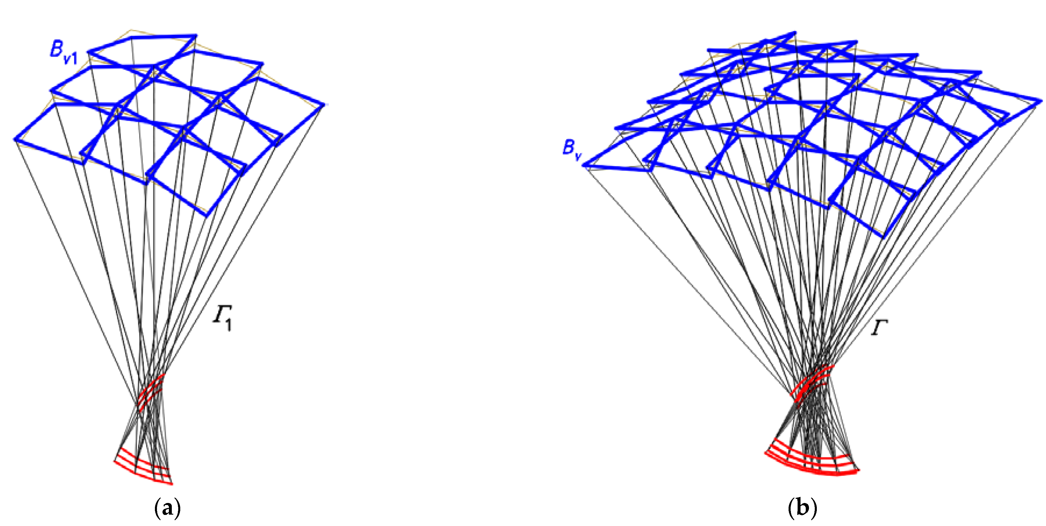
The first derivative configuration CP1 defines a discontinuous shell structure
Ω and a discontinuous polygonal network
Bv characterized by flat areas of discontinuity between the subsequent shell sectors
Ωij of
Ω (
Figure 11 and
Figure 14a,b). The discontinuous areas occurring between each pair of two adjacent meshes
Bvij and
Bvi+1j (
Ωij and
Ωi+1j) or
Bvij and
Bvij +1 (
Ωij and
Ωij+1) are the combinations of various triangles contained in the
Γ planes. For this configuration, all points
Aij and
Cij are located below
ω and all points
Bij and
Dij are located above
ω at the distances resulting from the respective values of the division coefficients d
Aij, d
Bij, d
Cij and d
Dij. The configuration CP1 is characterized by tetrads of the adjacent meshes
Bvij,
Bvi+1j,
Bvij+1 and
Bvi+1j+1 with two pairs of common vertices:
Cij =
Ai+1j+1 and
Bij+1 =
Di+1j located independently on the same side edge
cij =
bij+1 =
di+1j =
ai+1j+1 of
Γ.
The first spatial quadrangle
Bv11 is defined so that the points
A11 and
C11 lie on the side edges
a11 and
c11 below
ω and the points
B11 and
D11 above
ω at the distances used for the basic configuration CB and resulting from the adopted values of the following division coefficients: d
S11A11 = d
S11C11 = −0.1 and d
S11B11 = d
S11D11 = 0.1. The positions of two next meshes
Bv12 and
Bv21 are obtained by moving the points
A12,
B12,
C12,
D12,
A21,
B21,
C21 and
D21 of the configuration CB along the respective side edges of the
Γ network to their new positions
A12,
B12,
C12,
D12,
A21,
B21,
C21 and
D21 of the new configuration CP1 at the distances resulting from the values of the respective division coefficients adopted for
Bv and
Γ. The values of the coordinates of the vertices belonging to the quarter
Γ1 of the
z-axis-symmetric network
Γ calculated for CP1 are presented in
Table A8 in
Appendix A.
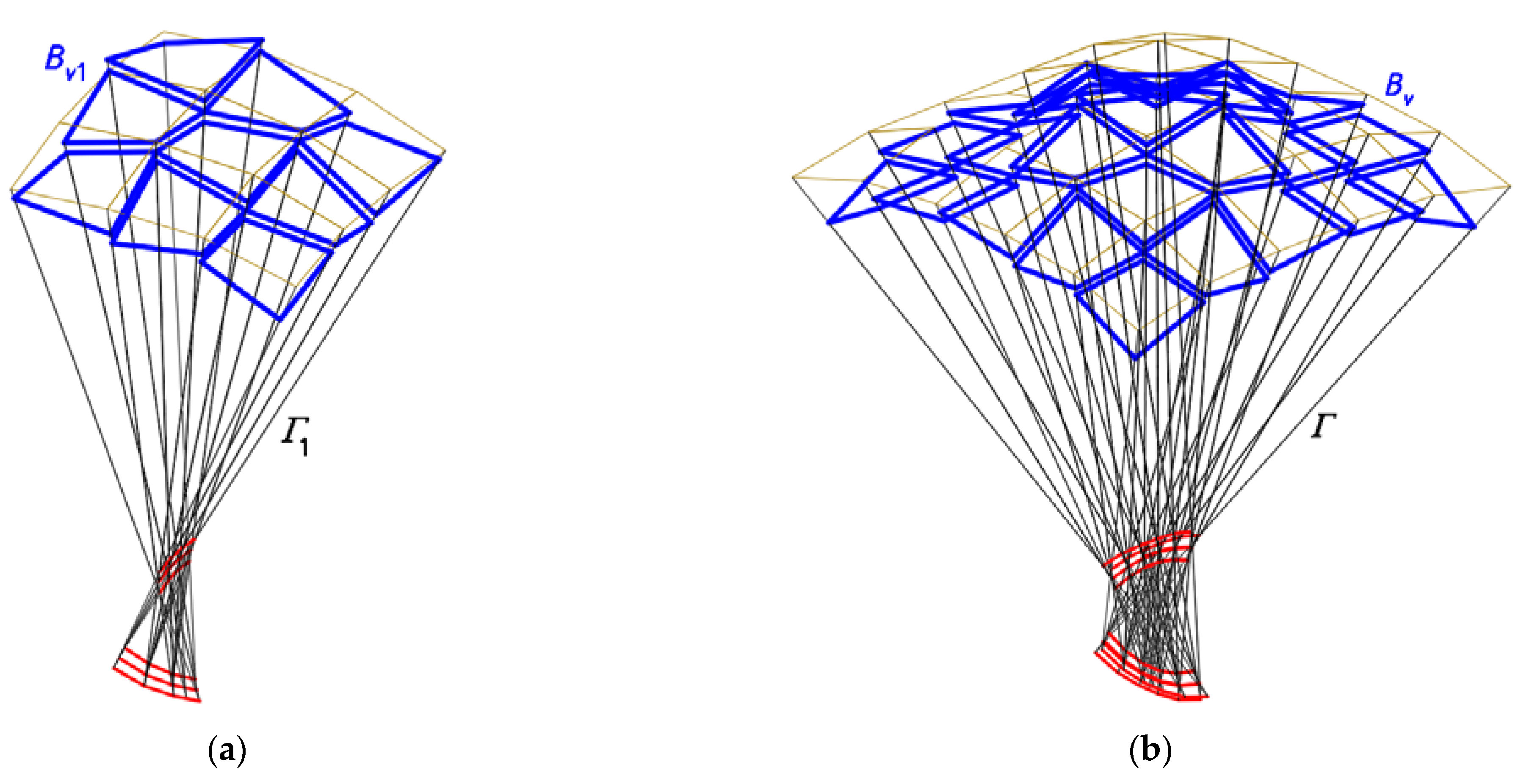
The second configuration CP2 derivative of CB is characterized by many flat quadrilateral areas of discontinuity between adjacent meshes
Bvij,
Bvi+1j,
Bvij+1 and
Bvi+1j+1 (
Figure 12 and
Figure 15). The locations of its vertices
Aij,
Bij,
Cij and
Dij defining the quadrangular areas of the
Ω discontinuity can be found as follows.
The first quadrangle
Bv11 is the same as for the basic configuration CB and derivative configuration CP1. The positions of two following quadrangles
Bv12 and
Bv21 are obtained by moving the points
A12,
B12,
C12,
D12,
A21,
B21,
C21 and
D21 of the configuration CB along the respective side edges of the
Γ network into their new positions
A12,
B12,
C12,
D12,
A21,
B21,
C21 and
D21 of the new configuration CP2 at the distances resulting from the values of the division coefficients d
S12A12, d
S12B12, d
S12C12 and d
S12D12, etc. The values of the coordinates of the vertices belonging to the quarter
Γ1 are presented in
Table A9 in
Appendix A.
The positions of the other vertices belonging to the subsequent new quadrangles Bv13, Bv22 Bv23, Bv32 and Bv31 of CP2 are obtained as a result of moving the points A13, B13, C13, D13, A22, B22, C22, D22, A23, B23, C23, D23, A31, B31, C31, D31, A32, B32, C32 and D32 of CB along the respective side edges of Γ into their new positions of CP2 resulting from the respective values of the division coefficients dSijAij, dSijBij, dSijCij and dSijDij for i = 1 and j = 3 or i = 3 and j = 1. In particular, the coefficients can be equal to twice or three times the value of the respective coefficient dS11A11 or dS11B11 or dS11C11 or dS11D11.
6. Discussion
All vertices Aij, Bij, Cij and Dij of the basic configuration CB are divided into two groups. The first group includes the vertices lying on one side of a reference surface ω, for example, above ω. The second group is composed of the other Bv vertices lying on the opposite side of ω, that is, under ω.
The positions of the sought-after vertices
Aij,
Bij,
Cij and
Dij lying on the side edges
aij,
bij,
cij and
dij of
Γ result from the adopted or calculated values of the division coefficients d
SAij, d
SBij, d
SCij and d
SDij. If we know the values of the above coefficients, the values the division coefficients d
Aij, d
Bij, d
Cij and d
Dij, required to calculate the positions of
Aij,
Bij,
Cij and
Dij, can be calculated as follows:
The values of the division coefficients d
Aij, d
Bij, d
Cij and d
Dij corresponding to the vertices of CB can be calculated with Equation (7) and the values are published in
Table A1 and
Table A5 in
Appendix A.
In the case of the investigated basic configuration CB (
Figure 10 and
Figure 13), the first subset is composed of the points
Aij and
Cij located under
ω, whereas the second subset is composed of the other points
Aij and
Cij positioned above
ω. Similarly, some of the points
Bij and
Dij are located above
ω and others lie under
ω.
To divide the points
Aij and
Cij into two complementary subsets, the following formulas were developed. The points
Aij and
Cij are located under
ω if the subscripts
i and
j meet the following conditions:
or
or
where
kC is the integer constant corresponding to the examined mesh
Bvij. If Equations (8)–(10) related to the values of
i and
j of the respective mesh
Ωij are fulfilled, the points
Bij and
Dij are located above
ω. For example, if
kC = 0 and
j = 1, then
i = 3 and the points
A31 and
C31 lie below
ω and the points
B31 and
D31 lie above
ω. The same result is achieved when adopting
kc = 0 and
i = 1. For this case,
j = 3 and the points
A13 and
C13 lie below the surface
ω and the points
B13 and
D13 lie above
ω. If we use Equation (10) and
i =
j = 3, then we obtain the points
A33 and
C33 lying below
ω.
The points
Aij and
Cij take the positions above
ω and the points
Bij and
Dij lie under
ω if the following conditions are met:
or
For example, if kC = 0 and j = 1, then it follows from Equation (13) that i = 2 and the points A21 and C21 lie above ω, and the points B21 and D21 lie below ω. The same result is achieved when using Equation (12) and adopting kC = 0 and i = 1. In this case, j = 2 and the points A12 and C12 lie above ω, and the points B12 and D12 lie below ω.
The coefficients express the proportions between the diversity of the positions of the Bv vertices in relation to ω, and the diversity of the locations of the same vertices in relation to the Γ vertices. They allow one to describe and parameterize the form of not only the roof structure, but also the form of the entire building, including the attractiveness and proportions between its basic dimensions. In this case, the double division coefficients must relate to the base level of the designed building. The above issues go beyond the scope of the article.
Thus, each of four vertices of Bvij of each basic configuration CB is shared with three adjacent meshes. In the search for several discontinuous configurations derivative of the base configuration CB, it is advisable to analyze the number of the adjacent Bv meshes possessing a common vertex. Four, three, two or only one vertex may be shared by the mesh with four adjacent meshes. The order of the common vertices of the adjacent meshes also affects the diversification of the derivative configurations.
The first derivative configuration CP1 (
Figure 14) examined in the previous section is characterized by the fact that two
Bvij and
Bvi+1j+1 subsequent meshes of
Bv arranged in the diagonal directions have one common vertex. The meshes arranged in the orthogonal directions do not have such a common vertex, and the respective sides of two adjacent meshes are mutually rotated in the planes of
Γ.
The conditions determining the positions of the vertices belonging to each tetrad of the adjacent
Bv meshes of the configuration CP2 are adopted so that a complete separation of the common vertices of the basic configuration CB is achieved. Thus, no pair of the adjacent meshes of CP2 has common vertices, and one side of each pair of two adjacent
Bv meshes is displaced in the respective plane of
Γ. As a result, a discontinuous roof structure consisting of many single transformed shells
Ωij limited by the mutually rotated eaves
Bvij is built (
Figure 12 and
Figure 15). The displacement is accomplished by simultaneously moving two ends of the above side along the respective side edges of
Γ either in the directions of the respective
Γ vertices or in the opposite directions. This action causes the additional increments of the division coefficients d
SijAij, d
SijBij, d
SijCij and d
SijDij resulting from the movement to be of the same sign.
For the special case when the values of these increments are identical, it is necessary to consider the number of the modifications accomplished for the subsequent pairs of two adjacent
Bv meshes when transmitting from
Bv11 to the examined
Bvij. The transition from
Bv11 to
Bv23 requires three skips between
Bv11 and
Bv12,
Bv12 and
Bv13, and
Bv13 and
Bv23. Thus, in order to build a mesh
Bvij, the number
i +
j − 2 of the skips is required. If the values of the increments assigned to the division coefficients d
SAij, d
SBij, d
SCij and d
SDij of CP2 are equal to the same constant dd
ij, then the increments dd
Aij, dd
Bij, dd
Cij and dd
Dij used for the vertices
Aij,
Bij,
Cij and
Dij (in relation to the base configuration CB) can be calculated from the formula
where dd
ij is the arbitrary constant related to the abovementioned skips.
It should be noted that two selected vertices of each pair of the adjacent meshes of
Bv arranged in the diagonal directions (
Figure 15), for example,
Bv21 and
Bv12, have one common vertex. If we change the values of the coefficients d
SijAij, d
SijBij, d
SijCij and d
SijDij of all
Bvij to create the configuration CP2 (in relation to the basic configuration CB) using Equation (13), then we should obtain the identical location of the vertices of the adjacent diagonal meshes
Bvij and
Bvi-1j+1 only for the very specific mutual position of all vertices
WABij,
WCDij,
WBCij and
WADij of
Γ. In fact, it will not be possible to achieve the abovementioned property of CP2 if we change the positions of these vertices of
Γ. This issue goes beyond the scope of the article.


