
Examining Ferromagnetic Materials Subjected to a Static Stress Load Using the Magnetic Method


Abstract
:1. Introduction
- ▪
- the magnetic flux leakage method is based on observation of the magnetic flux distribution over the material surface [1]. The primary magnetic field source causes a magnetic flux in the material. A barrier to the secondary flux is any inhomogeneity in the material structure that has a significant reluctance value [2]. The flux leakage method allows us to assess the tested object’s surface and subsurface inhomogeneity [3]. The main advantages are high sensitivity, easiness of signal acquisition, and the possibility of automation [2,4]. However, this method also has some disadvantages, including sensitivity to material impurities and the need to magnetize the object [5];
- ▪
- the magnetic particle inspection method allows for the detection of both surface and subsurface heterogeneities [6]. First, the sample is exposed to an external magnetic field, whereby magnetic powder particles can be placed on the outer surface of the sample in two ways: during the magnetization or after switching the magnetic field source off. The magnetic flux dispersing on the inhomogeneities appears on the material’s surface and changes the distribution of the particles [7]. The resulting image contains foci of particles that indicate the material heterogeneities [8]. Instead of magnetic powder, a suspension liquid can also be used to enhance the inspection sensitivity. Nowadays, apart from traditional indicators such as magnetic powders and suspension liquids, GMR or Hall sensors are also applicable to the inspection. The magnetic particle method is a quick, inexpensive, and relatively uncomplicated inspection method that gives immediate indications of surface and near-surface defects.
- ▪
- the eddy current testing method is based on observing the flow path of the induced currents in the examined material [9]. The excitation magnetic field source induces eddy currents in the material. Disturbances in eddy current flow caused by inhomogeneities become apparent in the resultant field [10]. The advantages of testing with eddy currents are the high efficiency of detecting even the most minor defects, no need for direct access, and the penetration of many layers of material [11,12]. The main disadvantage of this method is that it only detects defects located not too deep under the surface due to the skin effect, which is especially strong in the case of ferromagnetic materials [13];
- ▪
- the Barkhausen noise method relies on observing the magnetization process, which causes the dipoles to rotate [14,15,16]. If the material contains inhomogeneities, the process of domain wall shifting will be disrupted. As a result, sudden magnetization changes induce voltage pulses, which become apparent and can be observed as Barkhausen noise [17,18]. The Barkhausen noise testing method may be beneficial in some cases because of its low cost, high reliability, and simplicity [19]. The method is especially useful for stress monitoring. However, it has also some drawbacks, such as limited sensitivity resulting from thermal effects [20];
- ▪
- the 3MA is an approach that combines features of four NDT methods: the Barkhausen noise, eddy current, incremental permeability, and harmonic analysis of magnetic field strength methods. Using several methods simultaneously reduces the likelihood of inconclusive inspection results [21];
- ▪
- the magnetic memory method is based on the measurement of the residual magnetization, which appears in the material under the influence of a stress load or external geomagnetic fields [22]. The residual magnetization is recorded using sensors and then analyzed to assess defects [23]. The advantages of this method are the possibility to detect failures at an early stage, the lack of a need to provide an external magnetic field, and its simplicity [24]. A significant drawback is that it generally can be used only as an auxiliary method because of its low accuracy [24];
- ▪
- the hysteresis loop observation method is another method aimed at localizing stress and heterogeneities. The microstructure of the ferromagnetic material strongly affects the hysteresis loop shape [25]. If the tested object is subjected to stress, the coercivity field and remanence induction values change due to the displacement of the dipoles separated by Bloch walls [26,27].
2. Materials and Methods
3. Results and Discussion
4. Conclusions
Author Contributions
Funding
Institutional Review Board Statement
Informed Consent Statement
Data Availability Statement
Conflicts of Interest
References
- Pitoňák, M.; Neslušan, M.; Minárik, P.; Čapek, J.; Zgútová, K.; Jurkovič, M.; Kalina, T. Investigation of Magnetic Anisotropy and Barkhausen Noise Asymmetry Resulting from Uniaxial Plastic Deformation of Steel S235. Appl. Sci. 2021, 11, 3600. [Google Scholar] [CrossRef]
- Zhang, J.; Peng, F.; Chen, J. Quantitative Detection of Wire Rope Based on Three-Dimensional Magnetic Flux Leakage Color Imaging Technology. IEEE Access 2020, 8, 104165–104174. [Google Scholar] [CrossRef]
- Shimin, P.; Donglai, Z.; Enchao, Z. Analysis of the Eccentric Problem of Wire Rope Magnetic Flux Leakage Testing. In Proceedings of the 2019 IEEE 3rd Information Technology, Networking, Electronic and Automation Control Conference (ITNEC 2019), Chengdu, China, 15–17 March 2019. [Google Scholar] [CrossRef]
- Shi, Y.; Zhang, C.; Li, R.; Cai, M.; Jia, G. Theory and Application of Magnetic Flux Leakage Pipeline Detection. Sensors 2015, 15, 31036–31055. [Google Scholar] [CrossRef] [PubMed]
- Tsukada, K.; Yoshioka, M.; Toshihiko, K.; Joshinobu, H. A magnetic flux leakage method using a magnetoresistive sensor for nondestructive evaluation of spot welds. NDT Int. 2011, 44, 101–105. [Google Scholar] [CrossRef]
- Wong, B.S.; Low, Y.G.; Wang, X.; Ho, J.; Tan, C.H.; Boon, O.J. 3D Finite Element Simulation of Magnetic Particle Inspection. In Proceedings of the 2010 IEEE Conference on Sustainable Utilization and Development in Engineering and Technology, Kuala Lumpur, Malaysia, 20–21 November 2010; pp. 50–55. [Google Scholar] [CrossRef]
- Mouritz, A.P. Nondestructive Inspection and Structural Health Monitoring of Aerospace Materials. Introd. Aerosp. Mater. 2012, 534–557. [Google Scholar] [CrossRef]
- Wang, M.L.; Lynch, J.P.; Sohn, H. Sensing Solutions for Assessing and Monitoring Underwater Systems. Sens. Technol. Civ. Infrastruct. 2014, 525–549. [Google Scholar] [CrossRef]
- Xie, Y.; Li, J.; Tao, Y.; Wang, S.; Yin, W.; Xu, L. Edge Effect Analysis and Edge Defect Detection of Titanium Alloy Based on Eddy Current Testing. Appl. Sci. 2020, 10, 8796. [Google Scholar] [CrossRef]
- Socheatra, S. Printed Circuit Board Interconnect Fault Inspection Based on Eddy Current Testing. In Proceedings of the 2014 5th International Conference on Intelligent and Advanced Systems (ICIAS), Kuala Lumpur, Malaysia, 3–5 June 2014; pp. 1–4. [Google Scholar] [CrossRef]
- Repelianto, A.; Naoya, K. The Improvement of Flaw Detection by theConfiguration of Uniform Eddy Current Probes. Sensors 2019, 19, 397. [Google Scholar] [CrossRef] [PubMed] [Green Version]
- Neugebauer, R.; Drossel, W.G.; Mainda, P.; Roscher, H.J.; Wolf, K.; Kroschk, M. Sensitivity Analysis of Eddy Current Sensors Using Computational Simulation. In Proceedings of the Progress In Electromagnetics Research Symposium, Suzhou, China, 12–16 September 2011; pp. 441–445. [Google Scholar]
- Liu, S.; Yanhua, S.; Xiaoyuan, J.; Yihua, K. A Review of Wire Rope Detection Methods, Sensors and Signal Processing Techniques. J. Nondestruct. Eval. 2020, 39, 85. [Google Scholar] [CrossRef]
- Krkoška, L. Investigation of Barkhausen Noise Emission in Steel Wires Subjected to Different Surface Treatments. Coatings 2020, 10, 912. [Google Scholar] [CrossRef]
- Jurkovič, M.; Kalina, T.; Zgútová, K.; Neslušan, M.; Pitoňák, M. Analysis of Magnetic Anisotropy and Non-Homogeneity of S235 Ship Structure Steel after Plastic Straining by the Use of Barkhausen Noise. Materials 2020, 13, 4588. [Google Scholar] [CrossRef] [PubMed]
- Čilliková, M.; Mičietová, A.; Čep, R.; Mičieta, B.; Neslušan, M.; Kejzlar, P. Asymmetrical Barkhausen Noise of a Hard Milled Surface. Materials 2021, 14, 1293. [Google Scholar] [CrossRef] [PubMed]
- Prabhu, G.N.G.; Nlebedim, I.C.; Prabhu, G.G.V.; Jiles, D.C. Examining the Correlation Between Microstructure and Barkhausen Noise Activity for Ferromagnetic Materials. IEEE Trans. Magn. 2015, 51, 1–4. [Google Scholar] [CrossRef]
- Bui, T.M.T. Toward a Model of Barkhausen Noise Measurement System. In Proceedings of the 2011 International Conference on Advanced Technologies for Communications (ATC 2011), Da Nang, Vietnam, 2–4 August 2011; pp. 315–318. [Google Scholar] [CrossRef]
- Vourna, P.; Ktena, A.; Tsakiridis, P.E.; Hristoforou, E. An accurate evaluation of the residual stress of welded electrical steels with magnetic Barkhausen noise. Measurement 2015, 71, 31–45. [Google Scholar] [CrossRef]
- Franco, G.F.A.; Padovese, L.R. Non-destructive scanning for applied stress by the continuous magnetic Barkhausen noise method. J. Magn. Magn. Mater. 2018, 446, 231–238. [Google Scholar] [CrossRef]
- Wolter, B.; Gabi, Y.; Conrad, C. Nondestructive Testing with 3MA—An Overview of Principles and Applications. Appl. Sci. 2019, 9, 1068. [Google Scholar] [CrossRef] [Green Version]
- Zhang, Z. Wavelet Energy Entropy Based Multi-Sensor Data Fusion for Residual Stress Measurement Using Innovative Intense Magnetic Memory Method. In Proceedings of the 2009 9th International Conference on Electronic Measurement Instruments, Beijing, China, 16–19 August 2009; pp. 1044–1047. [Google Scholar] [CrossRef]
- Bao, S.; Fu, M.; Hu, S.; Gu, Y. A Review of the Metal Magnetic Memory Technique. In Proceedings of the ASME 2016 35th International Conference on Ocean, Offshore and Arctic Engineering, Busan, Korea, 19–24 June 2016. [Google Scholar]
- Wan, B. Research on the Damage Experiment Model Design and Metal Magnetic Memory Testing of Wind Turbine Tower in Service. In Proceedings of the 2020 IEEE 4th Conference on Energy Internet and Energy System Integration (EI2), Wuhan, China, 30 October–1 November 2020; pp. 1879–1884. [Google Scholar] [CrossRef]
- Fasheng, Q.; Wenwei, R.; Gui, Y.T.; Yunlai, G.; Bin, G. The effect of stress on the domain wall behavior of high permeability grain-oriented electrical steel. In Proceedings of the 2015 IEEE Far East NDT New Technology & Application Forum (FENDT), Zhuhai, China, 28–31 May 2015. [Google Scholar] [CrossRef]
- Liu, J.; Yun, T.G.; Gao, B.; Zeng, K.; Zheng, Y.; Chen, Y. Micro-Macro Characteristics between Domain Wall Motion and Magnetic Barkhausen Noise under Tensile Stress. J. Magn. Magn. Mater. 2020, 493, 165719. [Google Scholar] [CrossRef]
- Ding, S.; Tian, G.Y.; Dobmann, G.; Wang, P. Analysis of Domain Wall Dynamics Based on Skewness of Magnetic Barkhausen Noise for Applied Stress Determination. J. Magn. Magn. Mater. 2017, 421, 225–229. [Google Scholar] [CrossRef] [Green Version]
- Lee, Y.H.; Ji, W.; Kwon, D. Stress measurement of SS400 steel beam using the continuous indentation technique. Exp. Mech. 2004, 44, 55–61. [Google Scholar] [CrossRef]


| Parameter Definition | Parameter | Value |
|---|---|---|
| Excitation current RMS value | 400 mA | |
| Frequency of the excitation | 4.4 kHz | |
| Low-pass filter cutoff frequency | 50 kHz | |
| Amplifier gain | G | 30 dB |
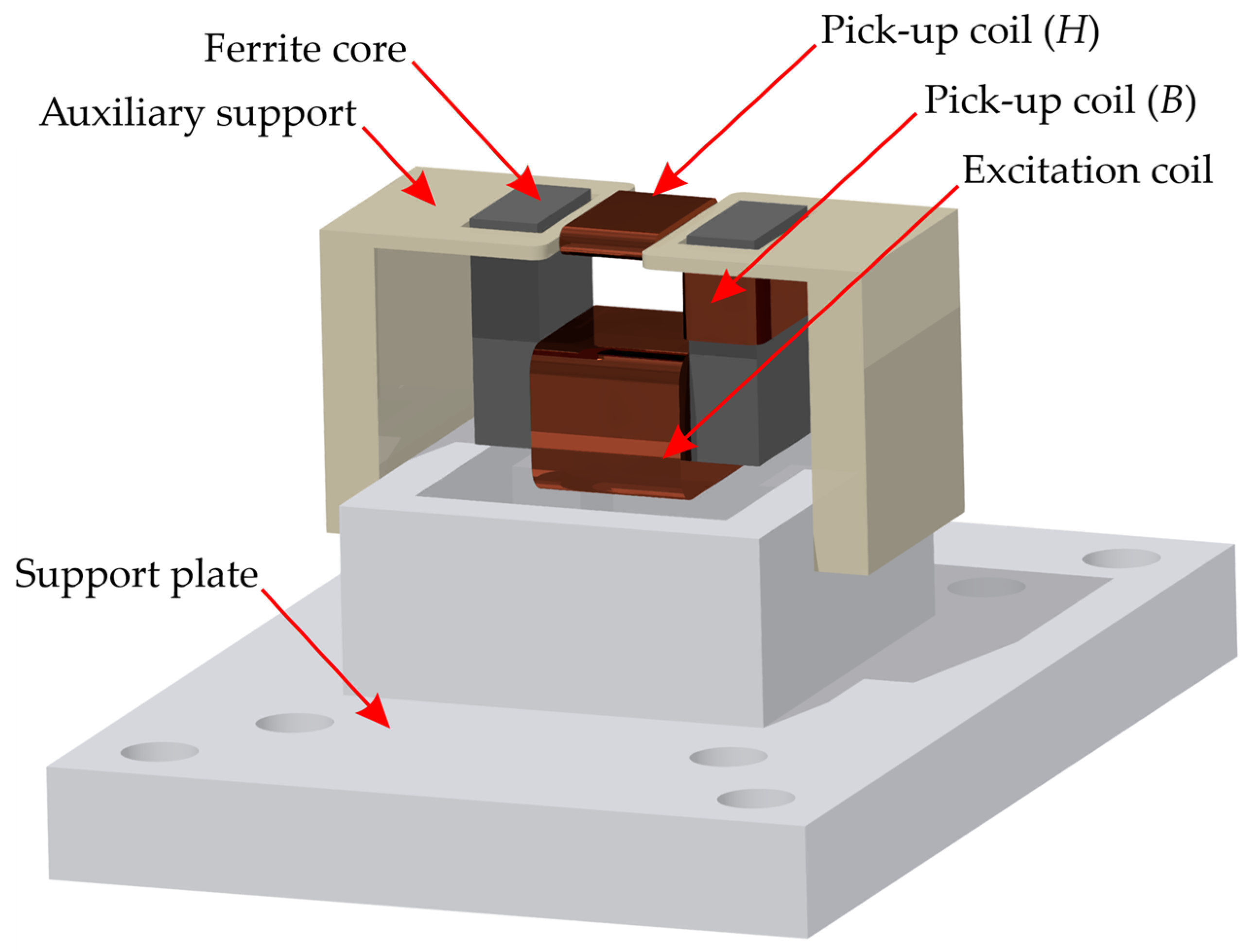
| Ferrite core length | 10.5 mm | |
| Ferrite core width | 5 mm | |
| Ferrite core height | 8.2 mm | |
| Pick-up coil (H) length | 3.2 mm | |
| Pick-up coil (H) width | 2 mm | |
| Pick-up coil (H) height | 4.75 mm | |
| Pick-up coil (H) number of turns | 90 | |
| Pick-up coil (B) length | 5 mm | |
| Pick-up coil (B) width | 2.5 mm | |
| Pick-up coil (B) height | 3 mm | |
| Pick-up coil (B) number of turns | . | 100 |
Publisher’s Note: MDPI stays neutral with regard to jurisdictional claims in published maps and institutional affiliations. |
© 2021 by the authors. Licensee MDPI, Basel, Switzerland. This article is an open access article distributed under the terms and conditions of the Creative Commons Attribution (CC BY) license (https://creativecommons.org/licenses/by/4.0/).
Share and Cite
Chady, T.; Łukaszuk, R. Examining Ferromagnetic Materials Subjected to a Static Stress Load Using the Magnetic Method. Materials 2021, 14, 3455. https://doi.org/10.3390/ma14133455
Chady T, Łukaszuk R. Examining Ferromagnetic Materials Subjected to a Static Stress Load Using the Magnetic Method. Materials. 2021; 14(13):3455. https://doi.org/10.3390/ma14133455
Chicago/Turabian StyleChady, Tomasz, and Ryszard Łukaszuk. 2021. "Examining Ferromagnetic Materials Subjected to a Static Stress Load Using the Magnetic Method" Materials 14, no. 13: 3455. https://doi.org/10.3390/ma14133455
APA StyleChady, T., & Łukaszuk, R. (2021). Examining Ferromagnetic Materials Subjected to a Static Stress Load Using the Magnetic Method. Materials, 14(13), 3455. https://doi.org/10.3390/ma14133455