Author Contributions
Conceptualization, Ł.P., Ł.R., R.K. and M.P.; methodology, Ł.P., Ł.R., R.K., M.P., M.W., D.B., W.Z. and V.P.; software, Ł.P., Ł.R., R.K., M.P., M.W., D.B., W.Z. and V.P.; validation, Ł.P., Ł.R., R.K. and M.P.; formal analysis, Ł.P., Ł.R., R.K. and M.P.; investigation, Ł.P., Ł.R., R.K., M.P., M.W., D.B., W.Z. and V.P.; resources, Ł.P., Ł.R., R.K., M.P., M.W., D.B., W.Z. and V.P.; data curation, Ł.P., Ł.R., R.K., M.P., M.W., D.B., W.Z. and V.P., writing of the original draft preparation, Ł.P., Ł.R., R.K. and M.P.; writing of review and editing, Ł.P., Ł.R., R.K. and M.P.; visualization, Ł.P., Ł.R., R.K. and M.P.; supervision, Ł.P., Ł.R., R.K. and M.P.; project administration, Ł.R., R.K. and M.P.; funding acquisition, R.K. and M.P. All authors have read and agreed to the published version of the manuscript.
Figure 1.
Schematic illustration of the investigated forgings with the locations of sensors: (a) adapter, (b) flange, (c) fork.
Figure 1.
Schematic illustration of the investigated forgings with the locations of sensors: (a) adapter, (b) flange, (c) fork.
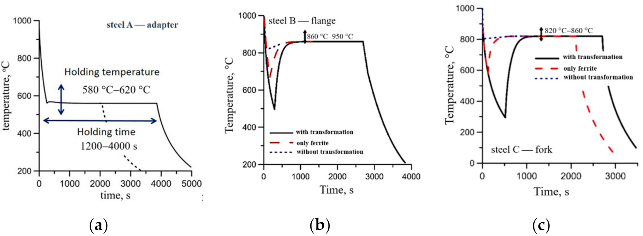
Figure 2.
Thermal cycles in points P during cooling of the investigated forgings: (a) annealing of the adapter, (b) normalization of the flange, (c) quenching and tempering of the fork.
Figure 2.
Thermal cycles in points P during cooling of the investigated forgings: (a) annealing of the adapter, (b) normalization of the flange, (c) quenching and tempering of the fork.
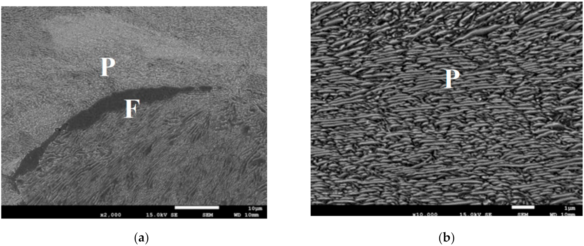
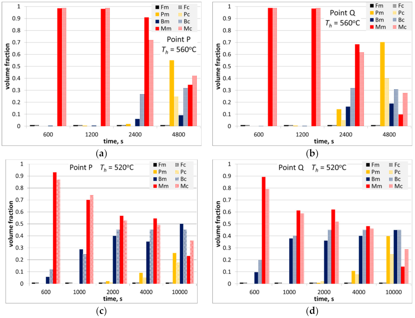
Figure 3.
(a,b) Selected microstructures of the samples after holding for 1 h at the temperature of 620 °C, various magnifications. P—pearlite; F—ferrite.
Figure 3.
(a,b) Selected microstructures of the samples after holding for 1 h at the temperature of 620 °C, various magnifications. P—pearlite; F—ferrite.
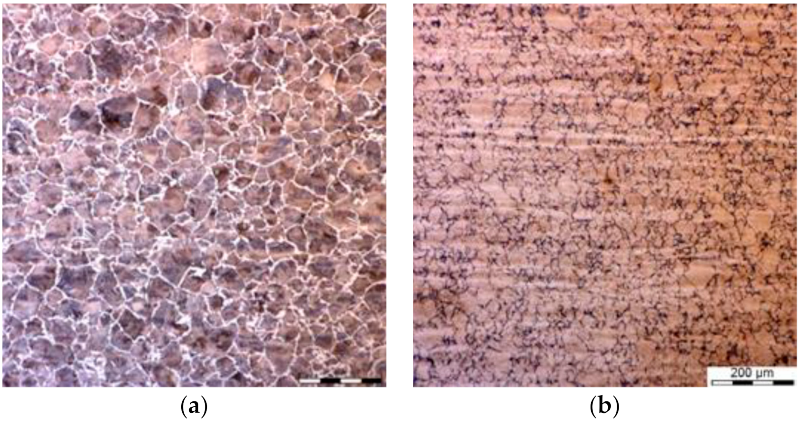
Figure 4.
Microstructures of the samples after holding at the temperature of 560 °C for 600 s (a), 1200 s (b), 2400 s (c) and 4000 s (d) F—ferrite, P—pearlite, B—bainite, M—martensite.
Figure 4.
Microstructures of the samples after holding at the temperature of 560 °C for 600 s (a), 1200 s (b), 2400 s (c) and 4000 s (d) F—ferrite, P—pearlite, B—bainite, M—martensite.
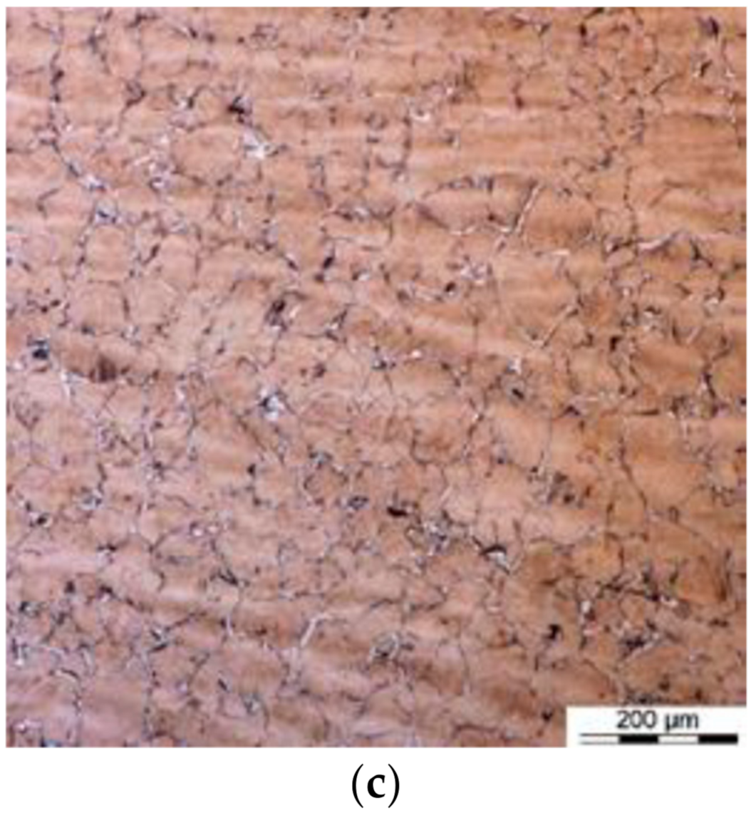
Figure 5.
Microstructures of the samples after holding at the temperature of 520 °C for 600 s (a), 1000 s (b), 2000 s (c) and 4000 s (d). F—ferrite, P—pearlite, B—bainite, M—martensite.
Figure 5.
Microstructures of the samples after holding at the temperature of 520 °C for 600 s (a), 1000 s (b), 2000 s (c) and 4000 s (d). F—ferrite, P—pearlite, B—bainite, M—martensite.
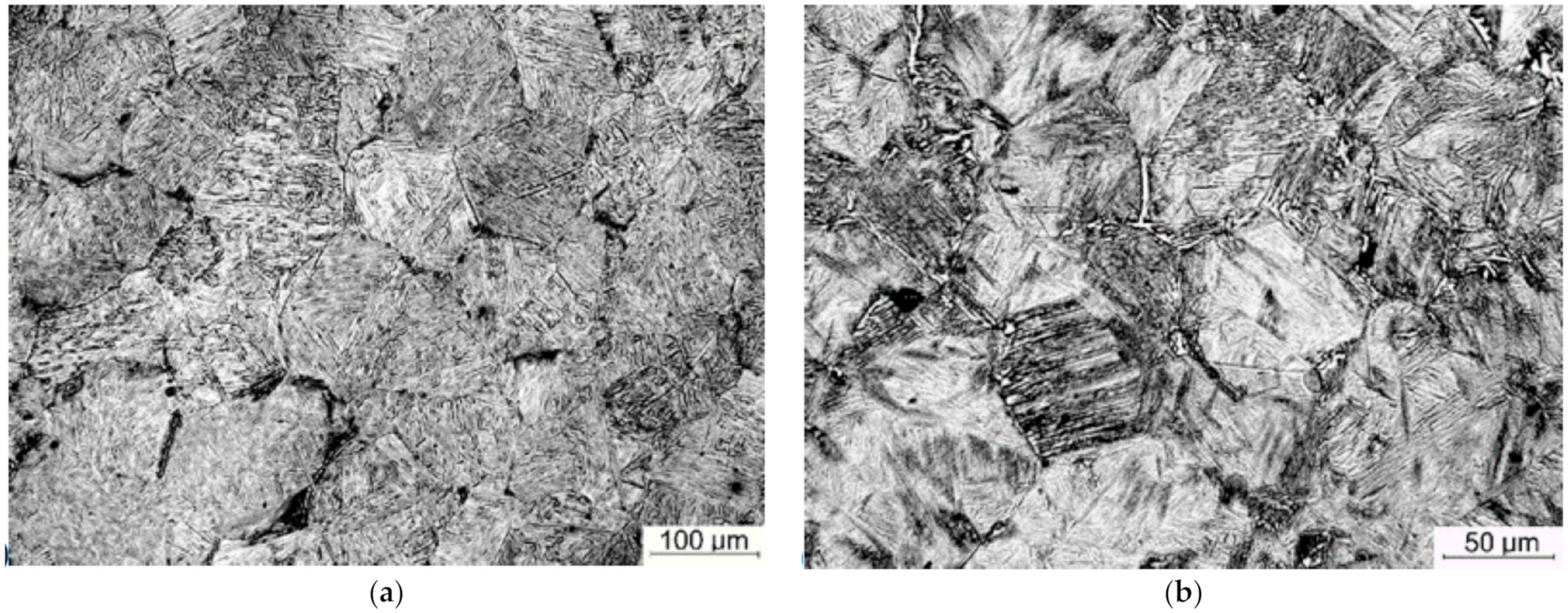
Figure 6.
Microstructures of steel B before the first deformation (a) and after the last deformation (b).
Figure 6.
Microstructures of steel B before the first deformation (a) and after the last deformation (b).
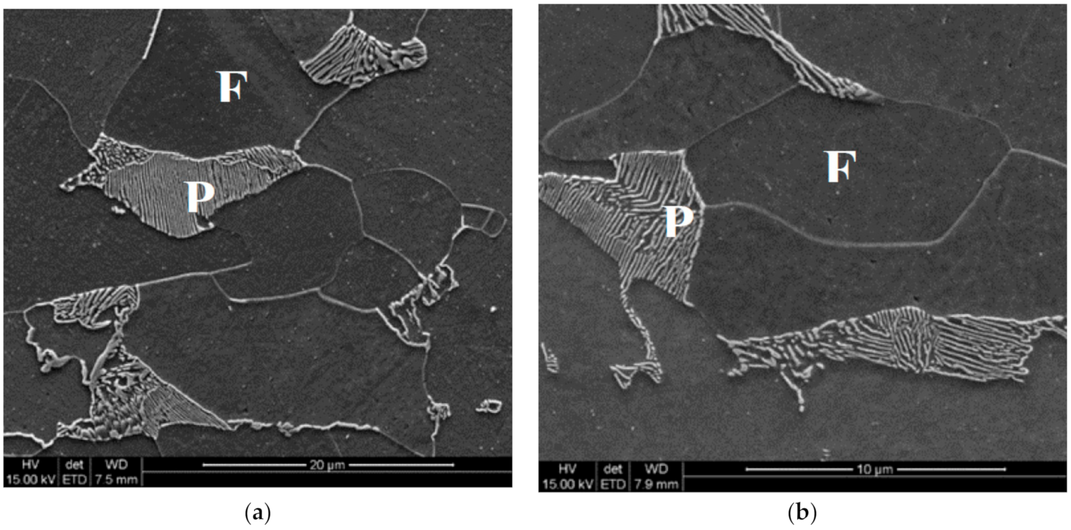
Figure 7.
Microstructures of steel B in point P after cooling variant 1 (a) and variant 0 (b). F—ferrite, P—pearlite.
Figure 7.
Microstructures of steel B in point P after cooling variant 1 (a) and variant 0 (b). F—ferrite, P—pearlite.
Figure 8.
Microstructures of steel C before the first deformation.
Figure 8.
Microstructures of steel C before the first deformation.
Figure 9.
Point P variant 1—microstructures of the samples after first cooling to 540 °C (a), after heating to the holding temperature (b) and at the end of holding (c).
Figure 9.
Point P variant 1—microstructures of the samples after first cooling to 540 °C (a), after heating to the holding temperature (b) and at the end of holding (c).
Figure 10.
Point P variant 2—microstructures of the samples after first cooling to 670 °C (a), after heating to the holding temperature (b) and at the end of holding (c).
Figure 10.
Point P variant 2—microstructures of the samples after first cooling to 670 °C (a), after heating to the holding temperature (b) and at the end of holding (c).
Figure 11.
Point Q variant 1—microstructures of the samples after first cooling to 500 °C (a), after heating to the holding temperature (b) and at the end of holding (c).
Figure 11.
Point Q variant 1—microstructures of the samples after first cooling to 500 °C (a), after heating to the holding temperature (b) and at the end of holding (c).
Figure 12.
Point Q variant 2—microstructures of the samples after first cooling to 609 °C (a), after heating to the holding temperature (b) and at the end of holding (c).
Figure 12.
Point Q variant 2—microstructures of the samples after first cooling to 609 °C (a), after heating to the holding temperature (b) and at the end of holding (c).
Figure 13.
Measured and calculated austenite grain size at various stages of the process for steel B, EoF—end of forging.
Figure 13.
Measured and calculated austenite grain size at various stages of the process for steel B, EoF—end of forging.
Figure 14.
Measured and calculated austenite grain size at various stages of the process for steel C.
Figure 14.
Measured and calculated austenite grain size at various stages of the process for steel C.
Figure 15.
Measured (full symbols) and calculated (open symbols with lines) start and end temperatures of phase transformations in the CCT tests for steel B, grain size 30 ± 3 μm, (a) and steel C, grain size 37 ± 4 μm (a) and 51 ± 3 μm (c).
Figure 15.
Measured (full symbols) and calculated (open symbols with lines) start and end temperatures of phase transformations in the CCT tests for steel B, grain size 30 ± 3 μm, (a) and steel C, grain size 37 ± 4 μm (a) and 51 ± 3 μm (c).
Figure 16.
Measured and calculated volume fraction of phases in steel A after physical simulations described in
Section 3.3, holding temperature 560 °C (
a,
b) and 520 °C (
c,
d) in the massive part of the forging (
a,
c) and in the thinner part (
b,
d).
Figure 16.
Measured and calculated volume fraction of phases in steel A after physical simulations described in
Section 3.3, holding temperature 560 °C (
a,
b) and 520 °C (
c,
d) in the massive part of the forging (
a,
c) and in the thinner part (
b,
d).
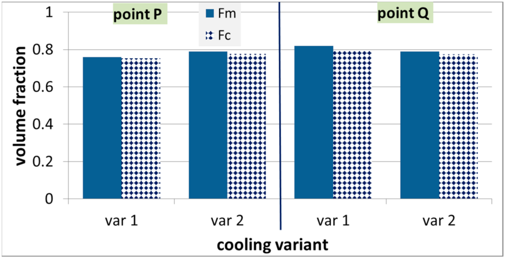
Figure 17.
Measured and calculated volume fraction of ferrite in steel B after physical simulations described in
Section 3.3.
Figure 17.
Measured and calculated volume fraction of ferrite in steel B after physical simulations described in
Section 3.3.
Figure 18.
Calculated distributions of the temperature (°C) (a) and austenite grain size (μm) (b) after forging of the adapter from steel A.
Figure 18.
Calculated distributions of the temperature (°C) (a) and austenite grain size (μm) (b) after forging of the adapter from steel A.
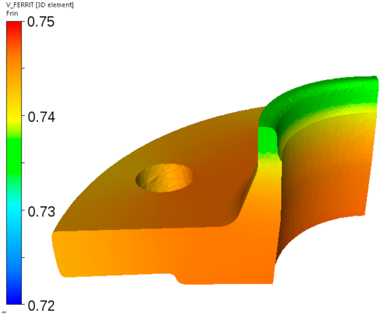
Figure 19.
Cooling of the adapter from steel A—calculated distributions of the pearlite volume fraction after holding at 560 °C for 1 h (a) and of the bainite volume fraction after holding at 520 °C for 1 h (b).
Figure 19.
Cooling of the adapter from steel A—calculated distributions of the pearlite volume fraction after holding at 560 °C for 1 h (a) and of the bainite volume fraction after holding at 520 °C for 1 h (b).
Figure 20.
Calculated distributions of the temperature (a) and austenite grain size (b) after forging of the flange from steel B.
Figure 20.
Calculated distributions of the temperature (a) and austenite grain size (b) after forging of the flange from steel B.
Figure 21.
Calculated distributions of the ferrite volume fraction after cooling of the flange from steel B according to the schedule in
Figure 2b.
Figure 21.
Calculated distributions of the ferrite volume fraction after cooling of the flange from steel B according to the schedule in
Figure 2b.
Figure 22.
Calculated distributions of the temperature (a) and austenite grain size (b) after forging of the fork from steel C.
Figure 22.
Calculated distributions of the temperature (a) and austenite grain size (b) after forging of the fork from steel C.
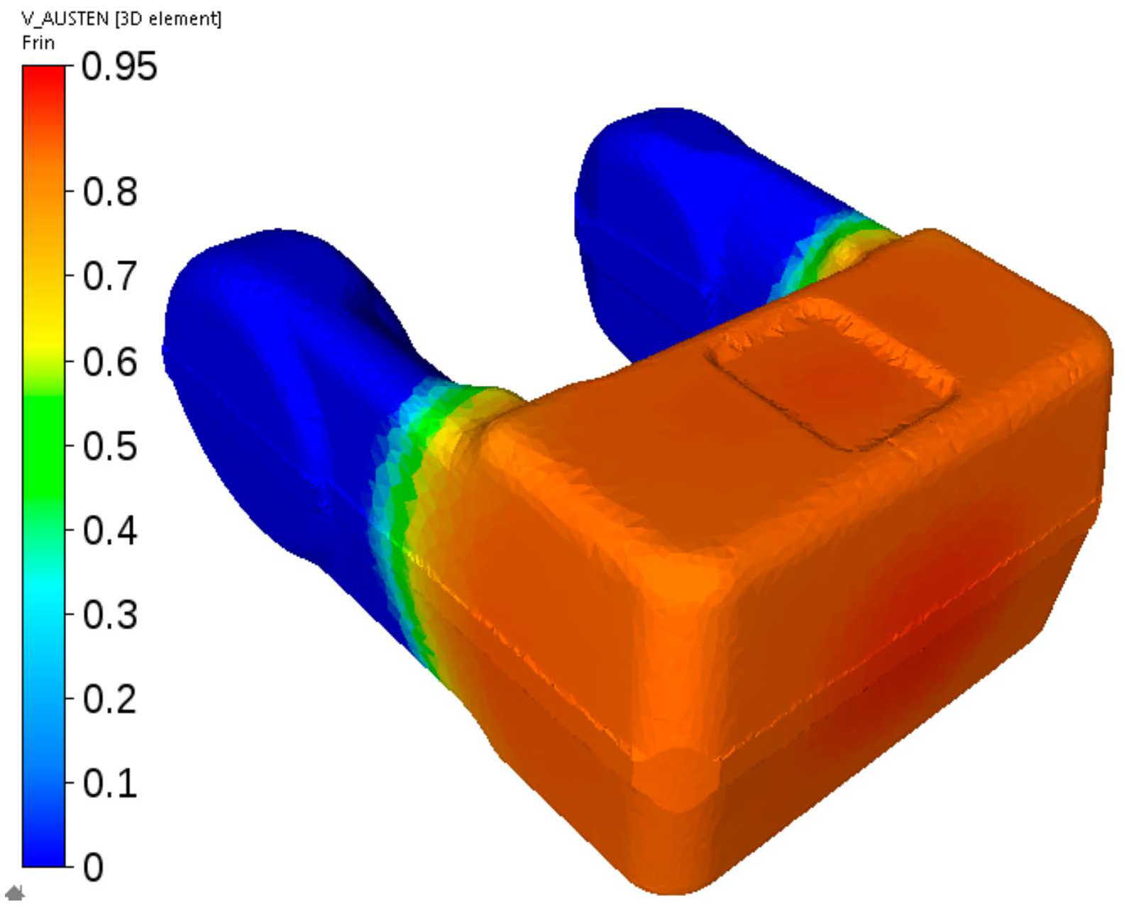
Figure 23.
First stage of the cooling of the fork from steel C—calculated distribution of the austenite volume fraction after cooling to the temperature at which ferritic transformation is completed and pearlitic transformation has not begun yet.
Figure 23.
First stage of the cooling of the fork from steel C—calculated distribution of the austenite volume fraction after cooling to the temperature at which ferritic transformation is completed and pearlitic transformation has not begun yet.
Table 1.
Equations describing microstructure evolution during hot forming.
Table 1.
Equations describing microstructure evolution during hot forming.
| Parameter | Equation |
|---|
| Kinetics of SRX |
| (1) |
| Grain size after SRX | | (2) |
| Critical strain for DRX | | (3) |
| DRX volume fraction | | (4) |
| Saturation strain | | (5) |
| Grain size after DRX | | (6) |
| Grain growth | | (7) |
Table 2.
Equations in the phase transformation models.
Table 2.
Equations in the phase transformation models.
| Parameter | Equation |
|---|
| Incubation time of perlite for the remaining transformation | | (9) |
| Incubation time of bainite for the remaining transformation | | (10) |
| Coefficients k for ferrite | | (11) |
| Coefficients k for perlite | | (12) |
| Coefficients k for bainite | | (13) |
| Average carbon content in austenite | | (14) |
| Bainite start temperatures | | (15) |
| Martensite start temperatures | | (16) |
| Martensite volume fraction | | (17) |
Table 3.
Chemical composition of the investigated steels, wt%.
Table 3.
Chemical composition of the investigated steels, wt%.
| Steel | C | Mn | Si | Cr | Ni | Cu | Mo |
|---|
| A | 0.42 | 0.744 | 0.237 | 1.049 | 0.122 | 0.209 | 0.171 |
| B | 0.18 | 0.58 | 0.17 | 0.39 | 0.1 | 0.24 | 0.02 |
| C | 0.48 | 0.58 | 0.23 | 0.12 | 0.16 | - | 0.04 |
Table 4.
Strains (ε) and temperatures (T, °C) in subsequent passes of physical simulation.
Table 4.
Strains (ε) and temperatures (T, °C) in subsequent passes of physical simulation.
| Part | Point | Pass 1 | Pass 2 | Pass 3 | Pass 4 |
|---|
| ε | T, °C | ε | T, °C | ε | T, °C | ε | T, °C |
|---|
| Adapter | P | 0.48 | 1229 | 0.52 | 1235 | 0.1 | 1232 | - | - |
| Q | 0.59 | 1228 | 0.89 | 1221 | 0.23 | 1211 | - | - |
| Flange | P | 0.4 | 1100 | 0.99 | 1103 | 0.07 | 1115 | - | - |
| Q | 0.64 | 1099 | 0.87 | 1106 | 0.06 | 1103 | - | - |
| Fork | P | 0.11 | 1125 | 0.95 | 1120 | 0.39 | 1101 | 0.3 | 1093 |
| Q | 0.12 | 1148 | 0.99 | 1147 | 1.69 | 1150 | 0.17 | 1120 |
Table 5.
Coefficients in microstructure equations for the investigated steels.
Table 5.
Coefficients in microstructure equations for the investigated steels.
| Coefficient | Steel A | Steel B | Steel C |
|---|
| n | 1.3025 | 1.4919 | 0.86 |
| a0 | 2.814 × 10⁻¹⁵ | 9.9684 × 10⁻¹³ | 2.199 × 10⁻¹⁶ |
| a1 | −1.4016 | −0.73206 | −1.0784 |
| a2 | −0.1195 | −0.15703 | −0.42 |
| a3 | 2.1793 | 3.9289 | 3.597 |
| QSRX | 244080 | 92147 | 186,000 |
| b0 | 0.6534 | 0.6143 | 28.713 |
| b1 | −0.2661 | −0.1017 | −0.3 |
| b2 | −0.06558 | −0.013 | −0.0796 |
| b3 | 1.1471 | 1.1683 | 0.1746 |
| QDSRX | 10,002 | 5008 | 6446 |
| p1 | 0.61928 × 10⁻³ | 1.9337 × 10⁻³ | 0.60634 × 10⁻⁴ |
| p2 | 0.2871 | 0.092 | 0.79995 |
| p3 | 0.1906 | 0.1814 | 0.18753 |
| p4 | 2.433 × 10⁻³ | 0.51143 × 10⁻³ | 0.5267 × 10⁻⁵ |
| p5 | 0.1481 | 0.5252 | 1.476 |
| p6 | 0.1951 | 0.1865 | 0.19823 |
| p7 | −1.4869 | −1.159 | −1.66863 |
| p8 | 1.8849 | 1.5158 | 1.62773 |
| p9 | 6822.71 | 3553 | 7676 |
| p10 | −0.1934 | −0.1837 | −0.21461 |
| QDEF | 284,798 | 278,878 | 280,204 |
| q | 8.34 | 7 | 5 |
| K | 4.3322 × 1030 | 4 × 1034 | 2.837 × 10¹⁶ |
| QGROWTH | 412,430 | 580,000 | 302,086 |
Table 6.
Optimal coefficients in the phase transformation model for steel A.
Table 6.
Optimal coefficients in the phase transformation model for steel A.
| a4 | a5 | a6 | a7 | a8 | a9 | a10 | a11 | a12 |
| 0.5417 | 0.74798 | 124.39 | 111.87 | 2.8367 | 6151.89 | 13.7849 | 1.118 | 666.76 |
| a13 | a14 | a15 | a16 | a17 | a18 | a19 | a20 | a21 |
| 350 | 1.072 | 2.1496 | 0.05 | 7.185 | 76.43 | 3.4748 | 574.998 | 300 |
| a22 | a23 | a24 | a25 | a26 | a27 | a28 | a29 | a30 |
| 236.55 | 10.2419 | 0.5 | 817.32 | 1299.8 | 0.011 | 0.0016 | 1.06559 | 1.2618 |
Table 7.
Optimal coefficients in the phase transformation model for steel B.
Table 7.
Optimal coefficients in the phase transformation model for steel B.
| a4 | a5 | a6 | a7 | a8 | a9 | a10 | a11 | a12 |
| 3.0 | 9.676 | 205.7 | 22.98 | 1.326 | 16.000 | 35.06 | 3.5 | 517 |
| a13 | a14 | a15 | a16 | a17 | a18 | a19 | a20 | a21 |
| 119 | 0.364 | 8.4 | 0.291 | 0.0167 | 9.804 | 0.168 | 569.8 | 378.7 |
| a22 | a23 | a24 | a25 | a26 | a27 | a28 | a29 | a30 |
| 61.66 | 10.86 | 0.5 | 362.1 | 0.047 | 0.011 | 0.516 | 0.636 | 0.927 |
Table 8.
Optimal coefficients in the phase transformation model for steel C.
Table 8.
Optimal coefficients in the phase transformation model for steel C.
| a4 | a5 | a6 | a7 | a8 | a9 | a10 | a11 | a12 |
| 1.33 | 5.896 | 185.7 | 75.85 | 2.713 | 16.000 | 12.54 | 3.5 | 594.9 |
| a13 | a14 | a15 | a16 | a17 | a18 | a19 | a20 | a21 |
| 47.29 | 0.664 | 18.19 | 0.487 | 0.309 | 0.012 | 0.1 | 535.4 | 498.13 |
| a22 | a23 | a24 | a25 | a26 | a27 | a28 | a29 | a30 |
| 15.63 | 13.2 | 3.7 | 656.7 | 696.4 | 0.011 | 1.3975 | 0.549 | 0.045 |

 ,
, 


