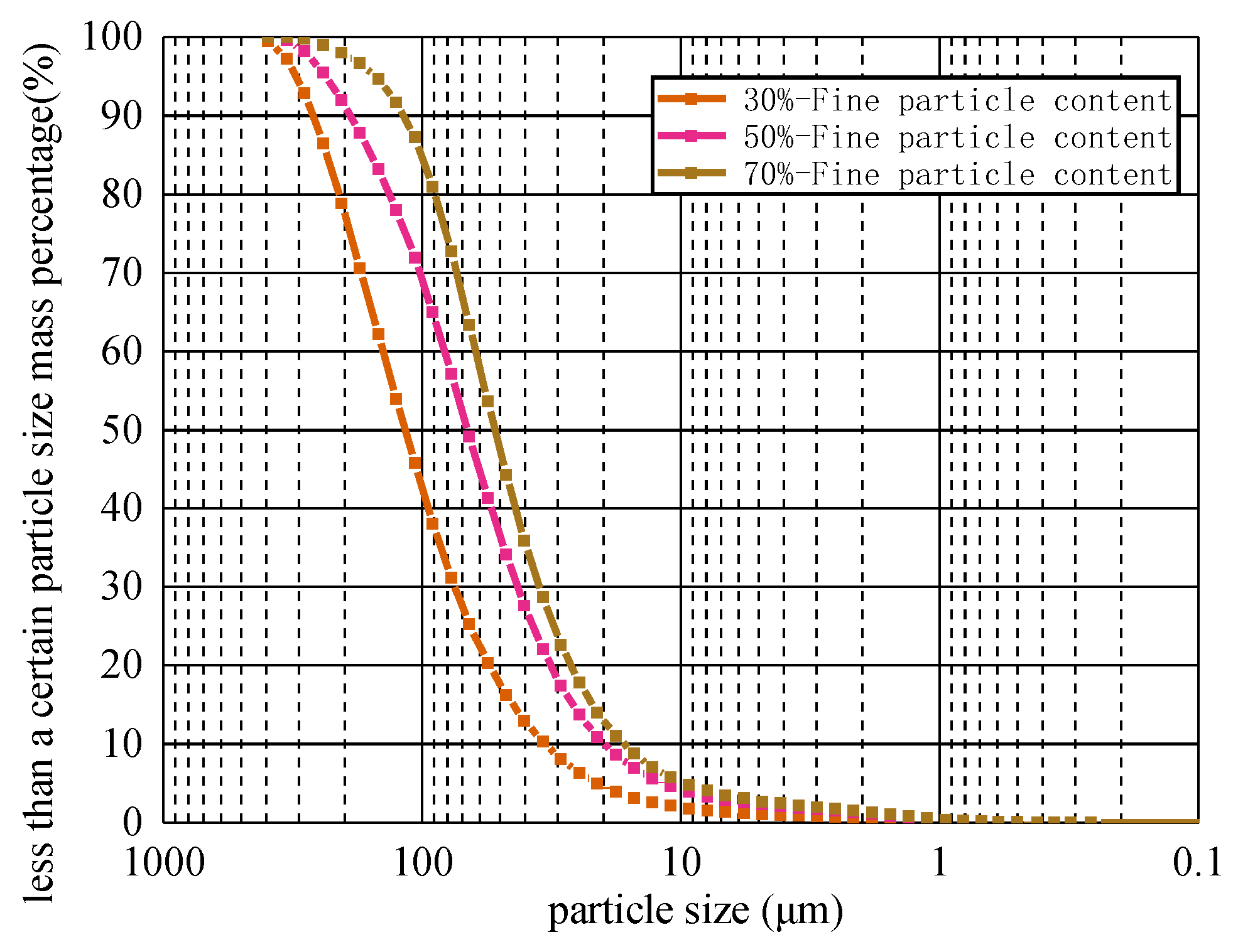
Figure 1.
Gradation curve of tailings sand.
Figure 1.
Gradation curve of tailings sand.
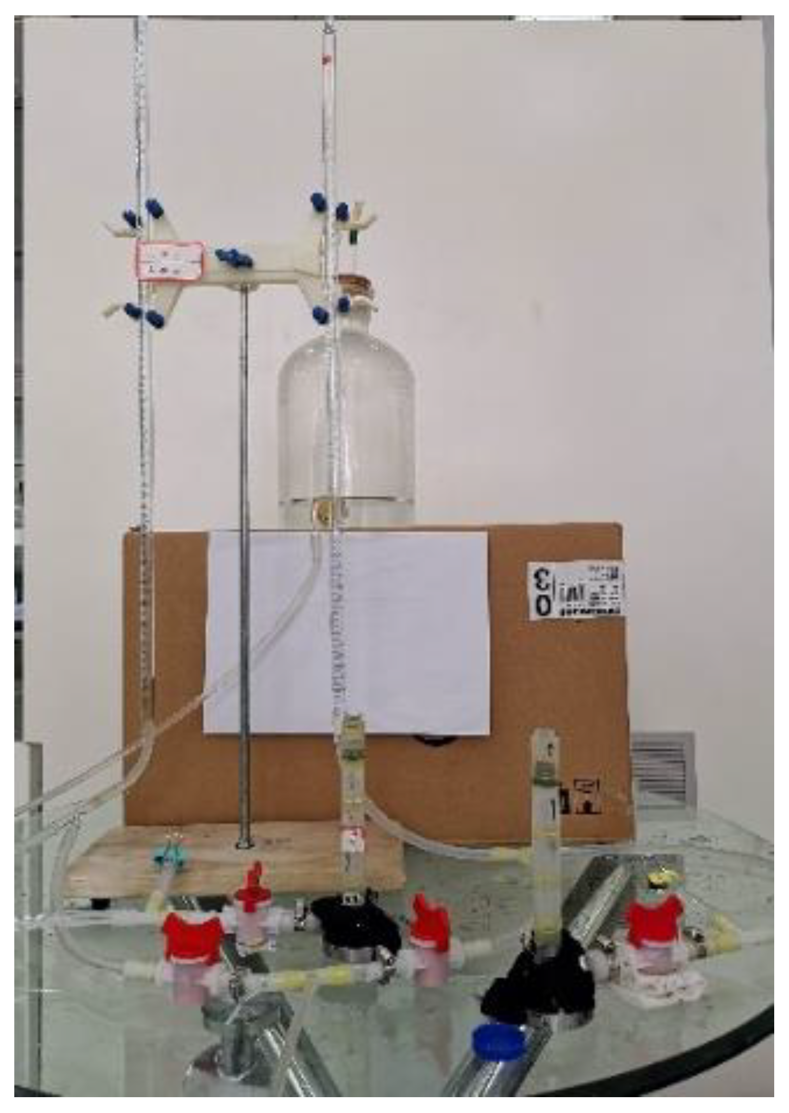
Figure 2.
Small osmotic deformation instrument.
Figure 2.
Small osmotic deformation instrument.
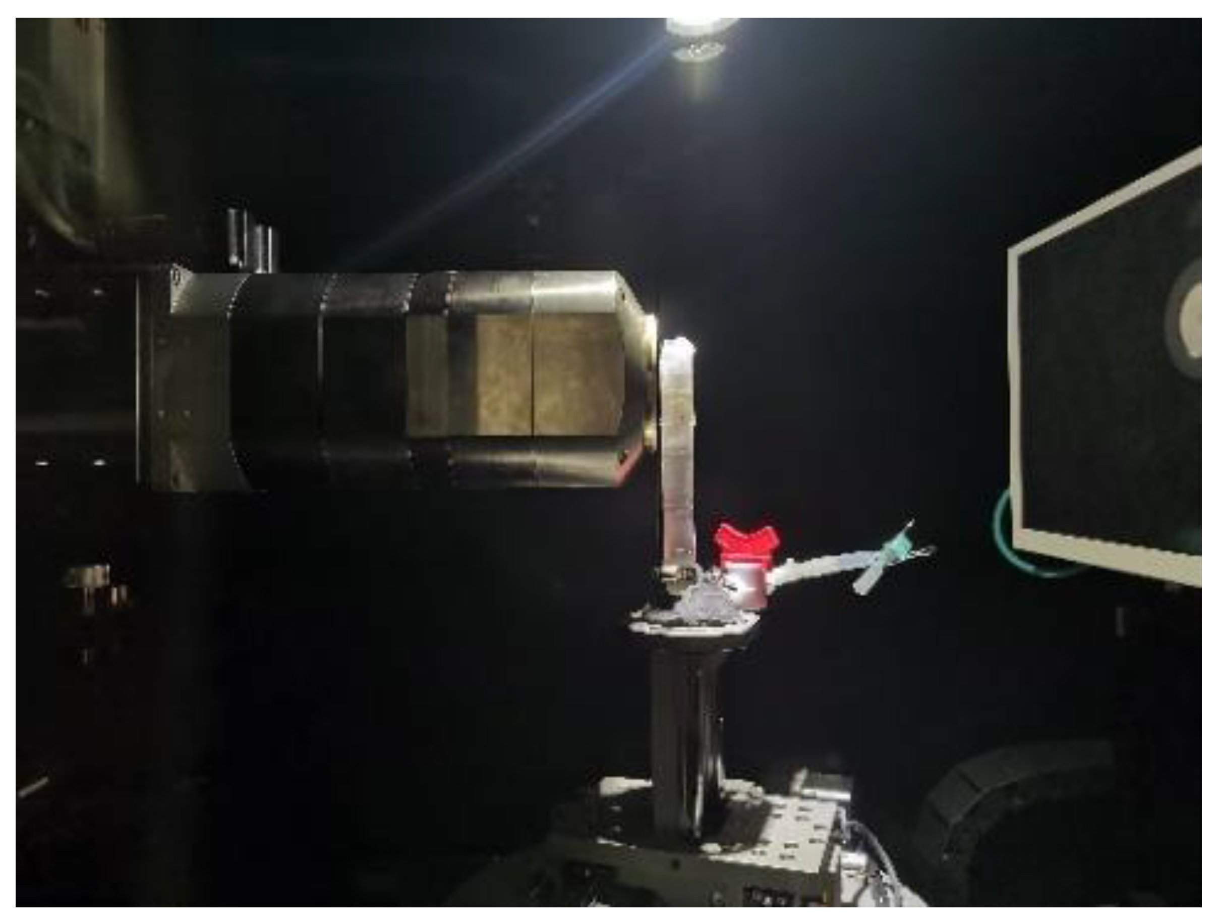
Figure 3.
nanoVoxel-3000 micro-CT.
Figure 3.
nanoVoxel-3000 micro-CT.
Figure 4.
CT scan of the tailings sand sample.
Figure 4.
CT scan of the tailings sand sample.
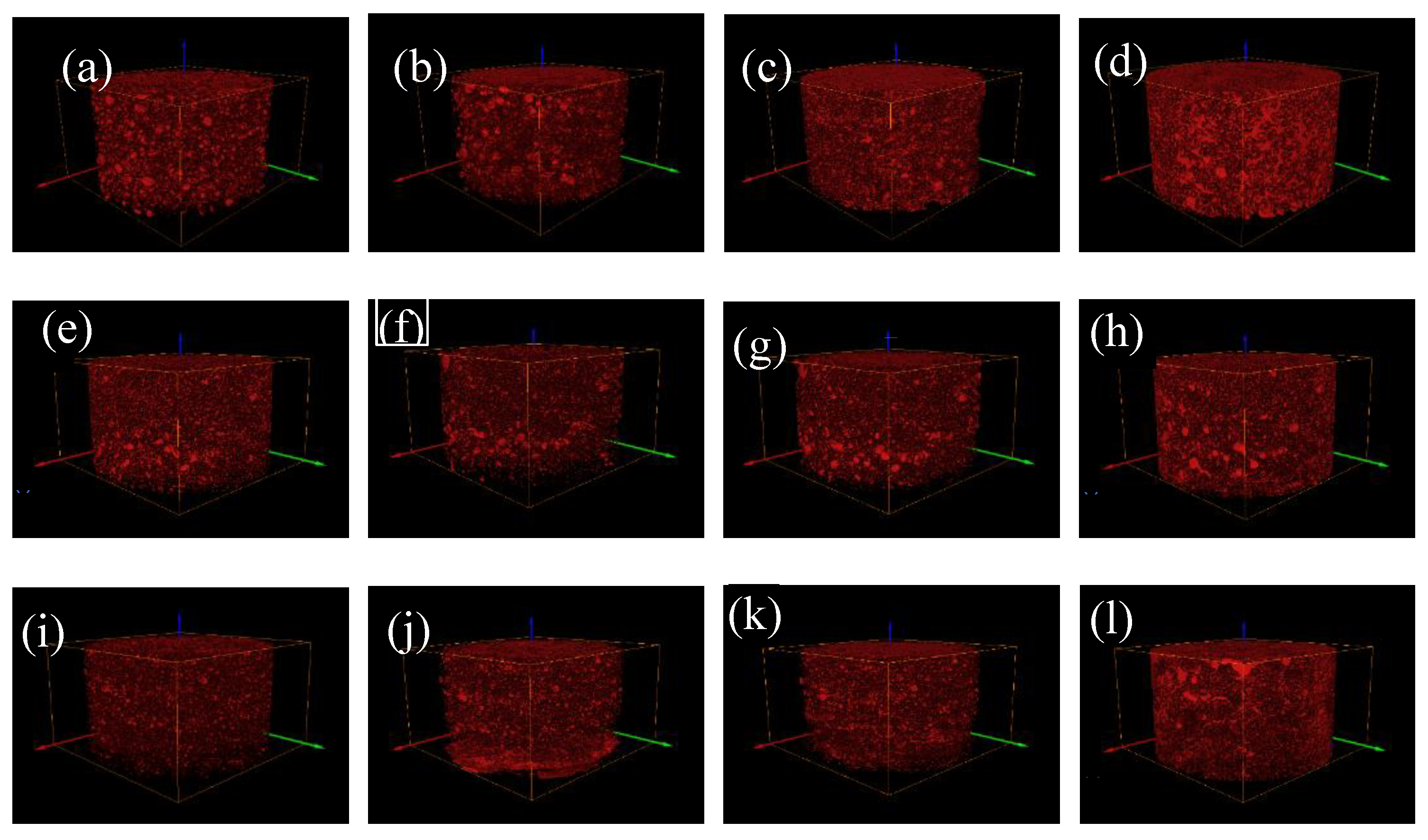
Figure 5.
Three-dimensional reconstruction of the three fine-grained tailings samples. (a) First-level head of 30% fine content; (b) Second-level head of 30% fine content; (c) Third-level head of 30% fine content; (d) Fourth-level head of 30% fine content; (e) First-level head of 50% fine content; (f) Second-level head of 50% fine content; (g) Third-level head of 50% fine content; (h) Fourth-level head of 50% fine content; (i) First-level head of 70% fine content; (j) Second-level head of 70% fine content; (k) Third-level head of 70% fine content; (l) Fourth-level head of 70% fine content.
Figure 6.
Pore threshold segmentation of the three fine-grained tailings sands. (a,b) First-level head of 30% fine content; (c,d) Second-level head of 30% fine content; (e,f) Third-level head of 30% fine content; (g,h) Fourth-level head of 30% fine content; (i,j) First-level head of 50% fine content; (k,l) Second-level head of 50% fine content; (m,n) Third-level head of 50% fine content; (o,p) Fourth-level head of 50% fine content; (q,r) First-level head of 70% fine content; (s,t) Second-level head of 70% fine content; (u,v) Third-level head of 70% fine content; (w,x) Fourth-level head of 70% fine content.
Figure 7.
The overall pore structure of the three fine-grained tailings sand samples. (a) First-level head of 30% fine content; (b) Second-level head of 30% fine content; (c) Third-level head of 30% fine content; (d) Fourth-level head of 30% fine content; (e) First-level head of 50% fine content; (f) Second-level head of 50% fine content; (g) Third-level head of 50% fine content; (h) Fourth-level head of 50% fine content; (i) First-level head of 70% fine content; (j) Second-level head of 70% fine content; (k) Third-level head of 70% fine content; (l) Fourth-level head of 70% fine content.
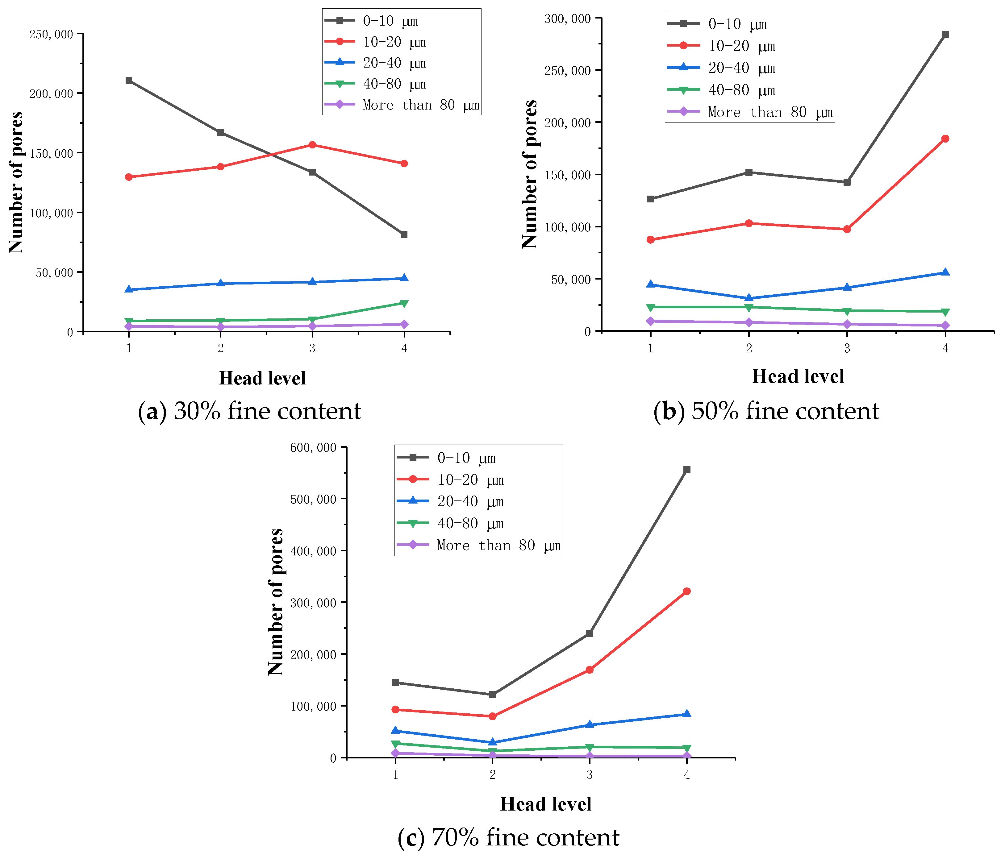
Figure 8.
Variation in the pore number. (a) 30% fine content; (b) 50% fine content; (c) 70% fine content.
Figure 8.
Variation in the pore number. (a) 30% fine content; (b) 50% fine content; (c) 70% fine content.
Figure 9.
Change in the total pore quantity.
Figure 9.
Change in the total pore quantity.
Figure 10.
Total connected pore volume change.
Figure 10.
Total connected pore volume change.
Figure 11.
Connected pore structure under three levels of the water content at the three levels of fine particle content. (a) First-level head of 30% fine content; (b) Second-level head of 30% fine content; (c) Third-level head of 30% fine content; (d) Fourth-level head of 30% fine content; (e) First-level head of 50% fine content; (f) Second-level head of 50% fine content; (g) Third-level head of 50% fine content; (h) Fourth-level head of 50% fine content; (i) Second-level head of 70% fine content; (j) Third-level head of 70% fine content; (k) Fourth-level head of 70% fine content.
Figure 12.
Layer-by-layer porosity statistics of the three fine-grained tailings sand samples.
Figure 12.
Layer-by-layer porosity statistics of the three fine-grained tailings sand samples.
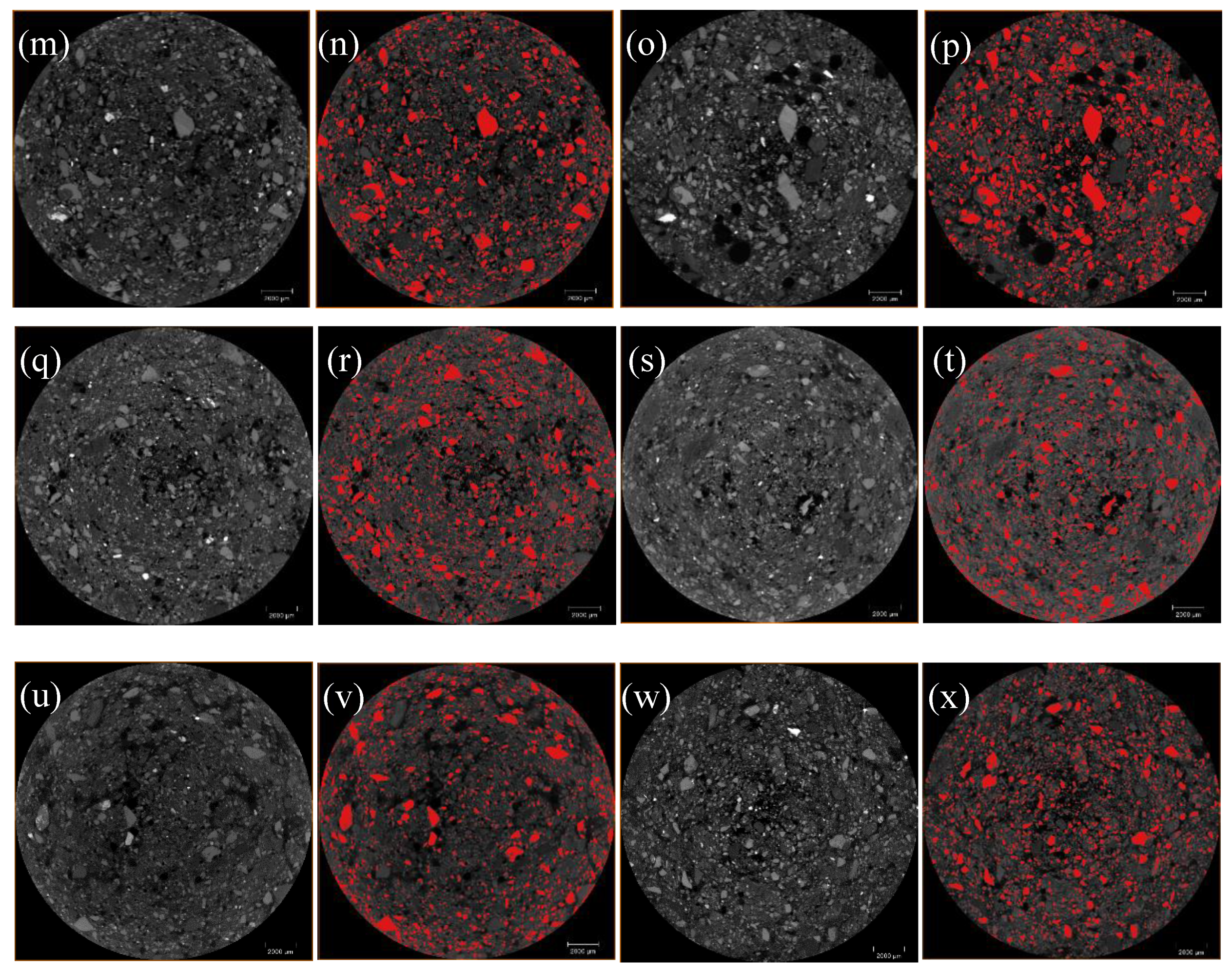
Figure 13.
Threshold segmentation of the tailings sand particles. (a,b) First-level head of the 30% fine content; (c,d) Second-level head of the 30% fine content; (e,f) Third-level head of the 30% fine content; (g,h) Fourth-level head of the 30% fine content; (i,j) First-level head of the 50% fine content; (k,l) Second-level head of the 50% fine content; (m,n) Third-level head of the 50% fine content; (o,p) Fourth-level head of the 50% fine content; (q,r) First-level head of the 70% fine content; (s,t) Second-level head of the 70% fine content; (u,v) Third-level head of the 70% fine content; (w,x) Fourth-level head of the 70% fine content.
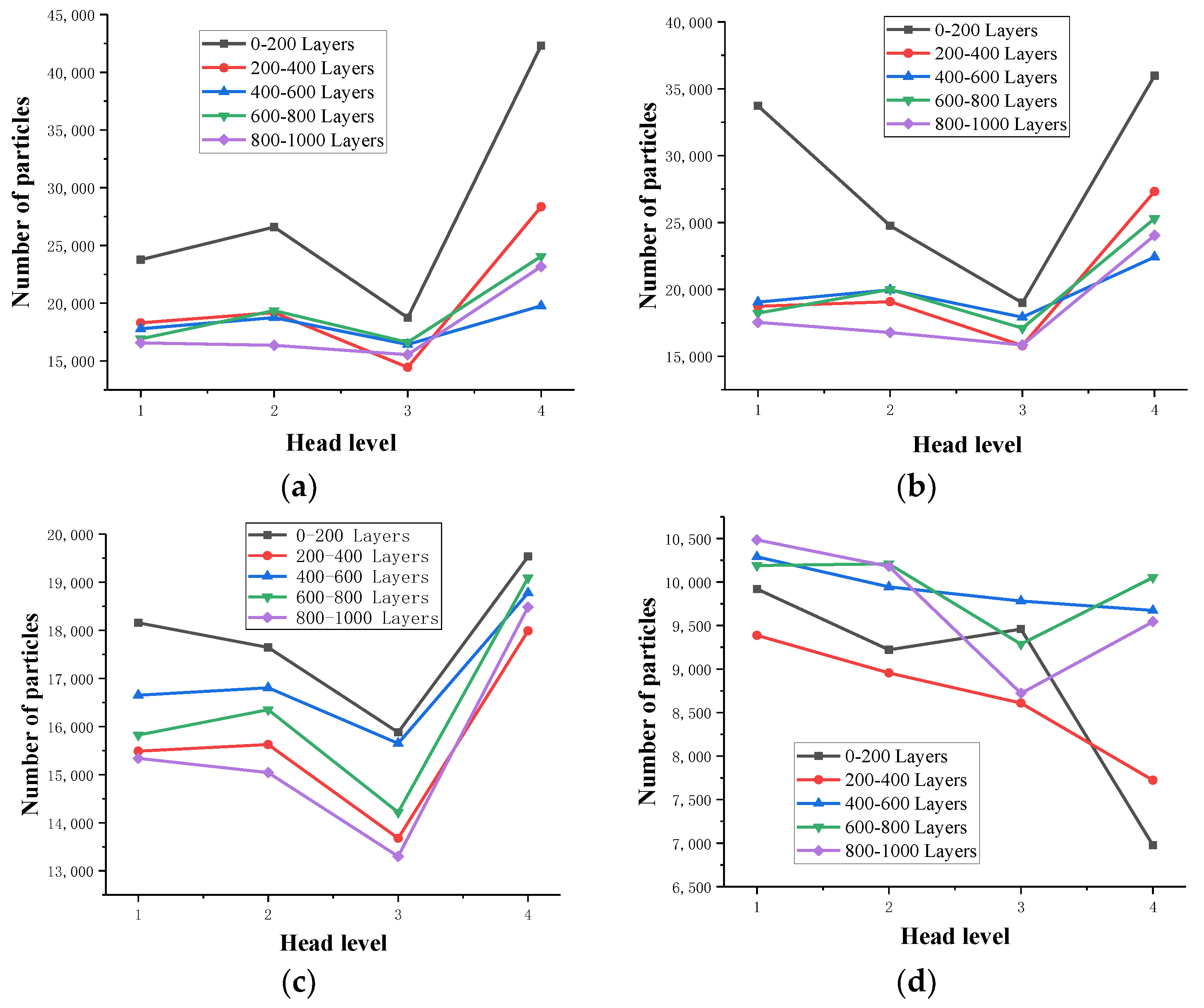
Figure 14.
Variation in the number of fine particles percolated with the 30% fine content. (a) Particle size: 0–10 µm; (b) Particle size: 10–20 µm; (c) Particle size: 20–40 µm; (d) Particle size: 40–75 µm.
Figure 14.
Variation in the number of fine particles percolated with the 30% fine content. (a) Particle size: 0–10 µm; (b) Particle size: 10–20 µm; (c) Particle size: 20–40 µm; (d) Particle size: 40–75 µm.
Figure 15.
Variation in the number of fine particles percolated with the 50% fine content. (a) Particle size: 0–10 µm; (b) Particle size: 10–20 µm; (c) Particle size: 20–40 µm; (d) Particle size: 40–75 µm.
Figure 15.
Variation in the number of fine particles percolated with the 50% fine content. (a) Particle size: 0–10 µm; (b) Particle size: 10–20 µm; (c) Particle size: 20–40 µm; (d) Particle size: 40–75 µm.
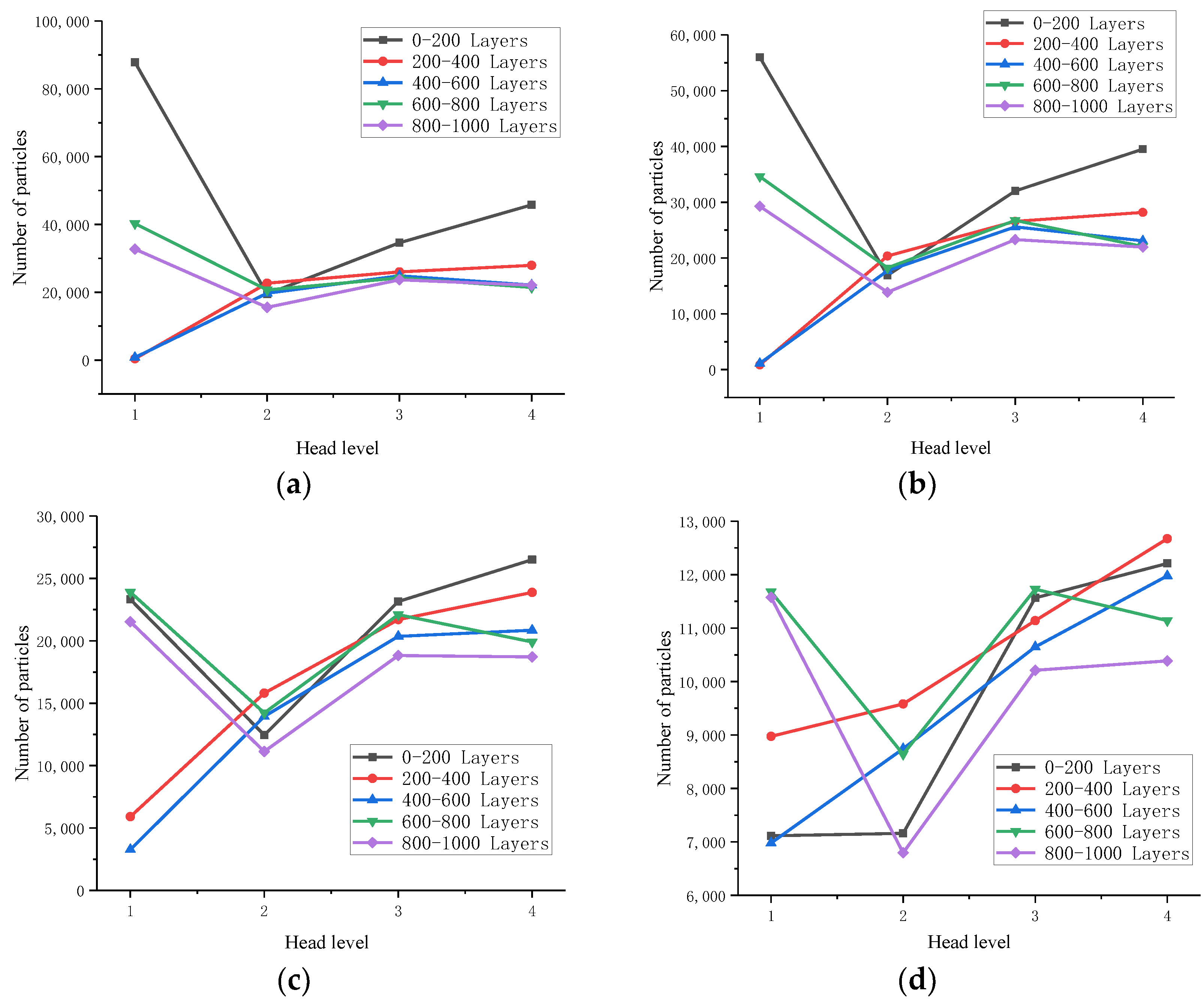
Figure 16.
Variation in the number of the fine particles percolated with the 70% fine content. (a) Particle size: 0–10 µm; (b) Particle size: 10–20 µm; (c) Particle size: 20–40 µm; (d) Particle size: 40–75 µm.
Figure 16.
Variation in the number of the fine particles percolated with the 70% fine content. (a) Particle size: 0–10 µm; (b) Particle size: 10–20 µm; (c) Particle size: 20–40 µm; (d) Particle size: 40–75 µm.
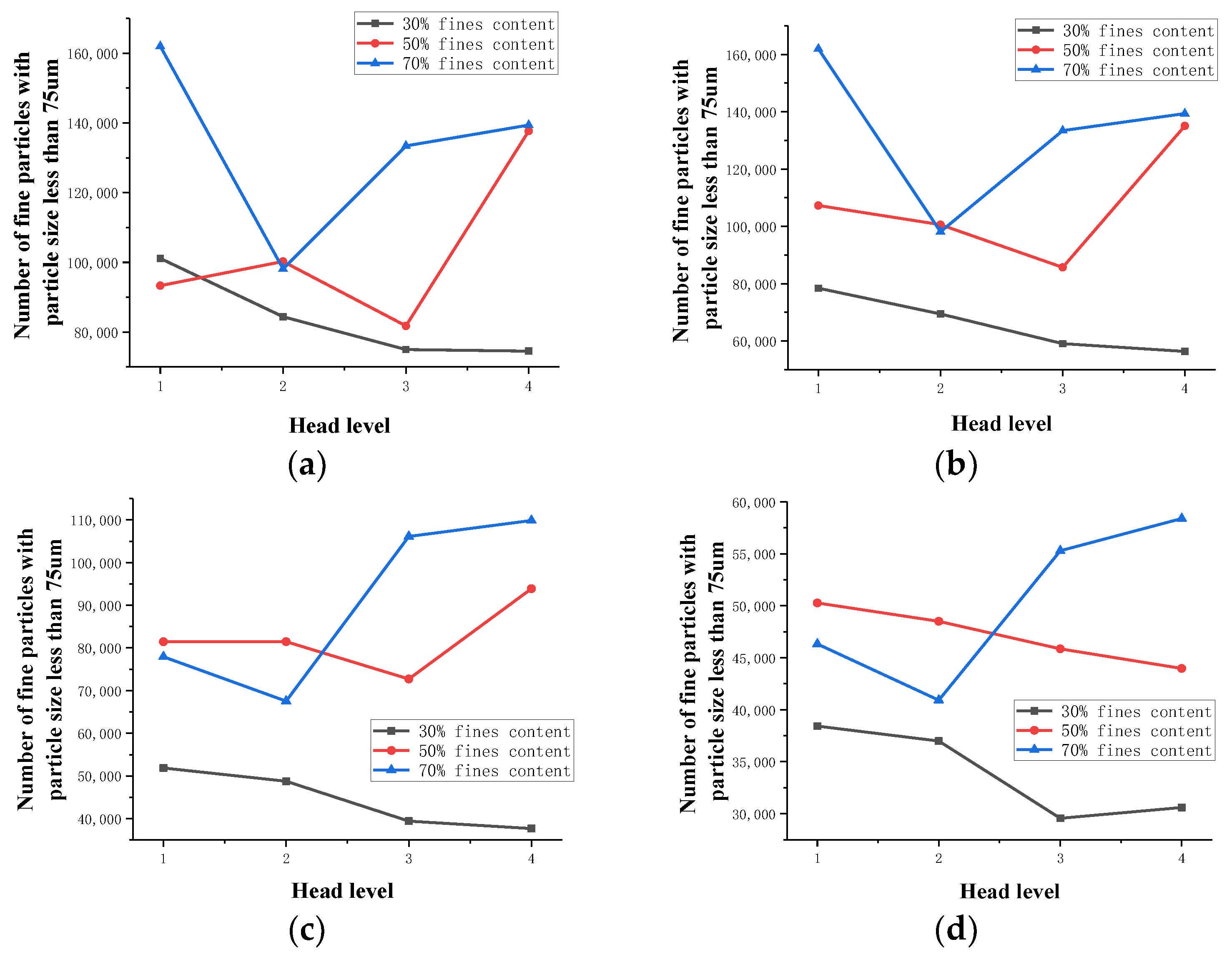
Figure 17.
The number of fine particles with different particle sizes. (a) 30% fine content; (b) 50% fine content; (c) 70% fine content.
Figure 17.
The number of fine particles with different particle sizes. (a) 30% fine content; (b) 50% fine content; (c) 70% fine content.
Figure 18.
Variation in the particle number during infiltration with different fine contents. (a) Particle size: 0–10 µm; (b) Particle size: 10–20 µm; (c) Particle size: 20–40 µm; (d) Particle size: 40–75 µm.
Figure 18.
Variation in the particle number during infiltration with different fine contents. (a) Particle size: 0–10 µm; (b) Particle size: 10–20 µm; (c) Particle size: 20–40 µm; (d) Particle size: 40–75 µm.
Figure 19.
Fine particle content as a function of the number of infiltration processes.
Figure 19.
Fine particle content as a function of the number of infiltration processes.
Figure 20.
Relationship between the proportion of the fine content and the initial content of fine particles.
Figure 20.
Relationship between the proportion of the fine content and the initial content of fine particles.
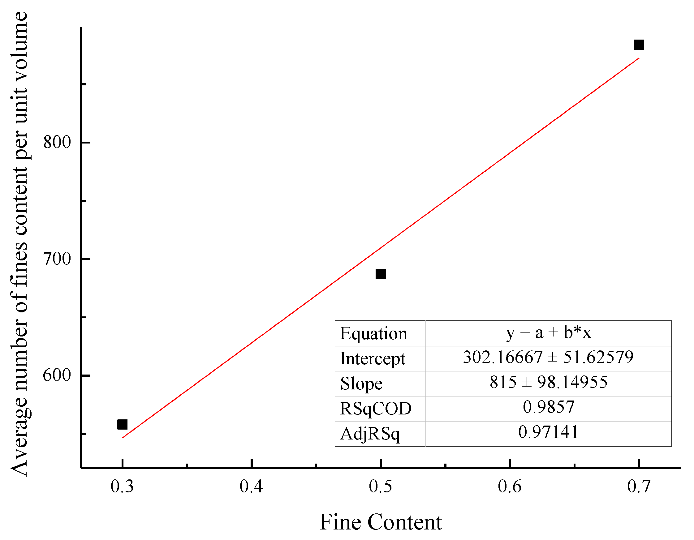
Figure 21.
Relationship between the proportion of the fine content and the average content of fine particles per unit volume.
Figure 21.
Relationship between the proportion of the fine content and the average content of fine particles per unit volume.
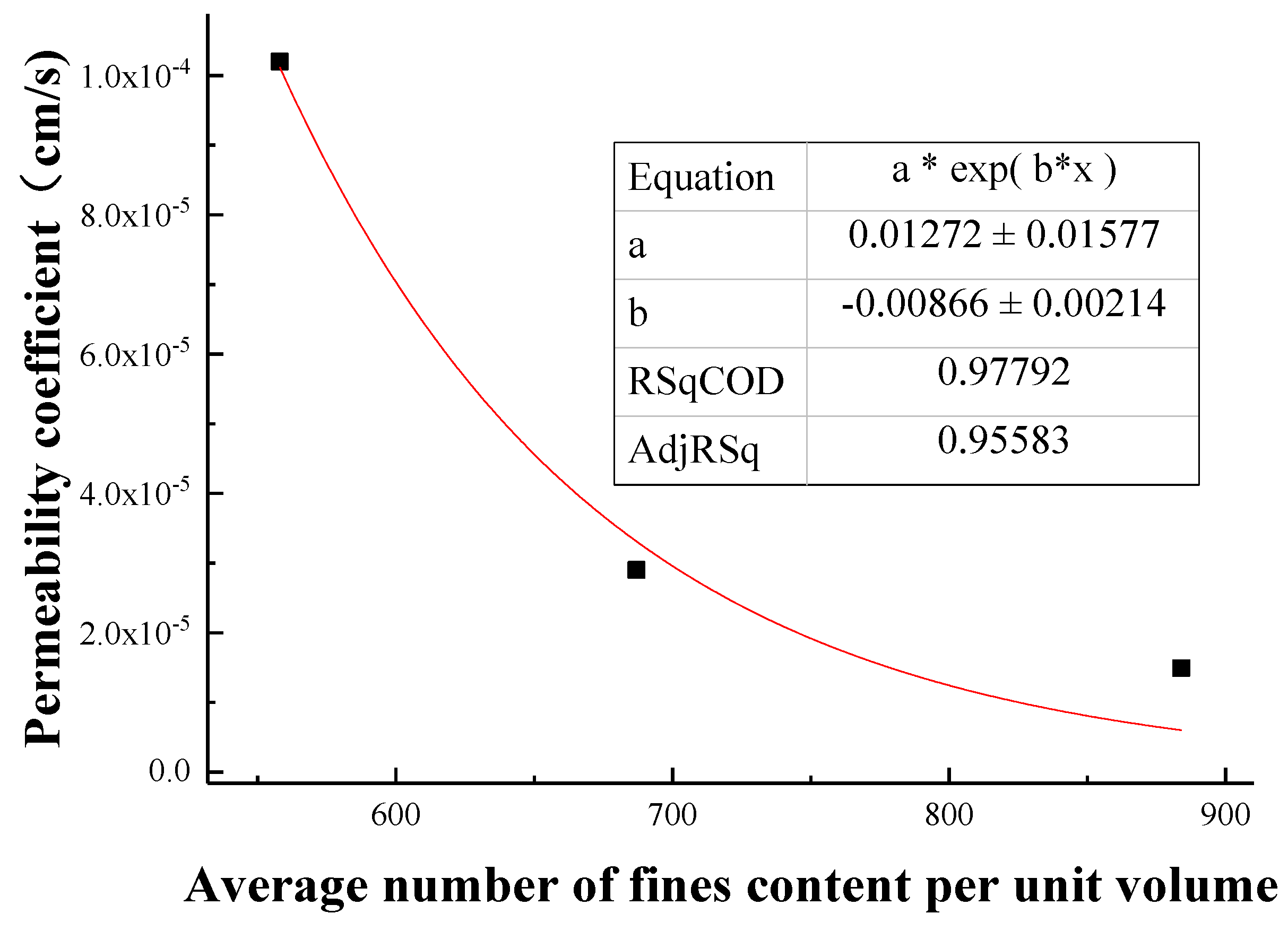
Figure 22.
Fitting curve of the fine particle content and permeability coefficient per unit volume.
Figure 22.
Fitting curve of the fine particle content and permeability coefficient per unit volume.
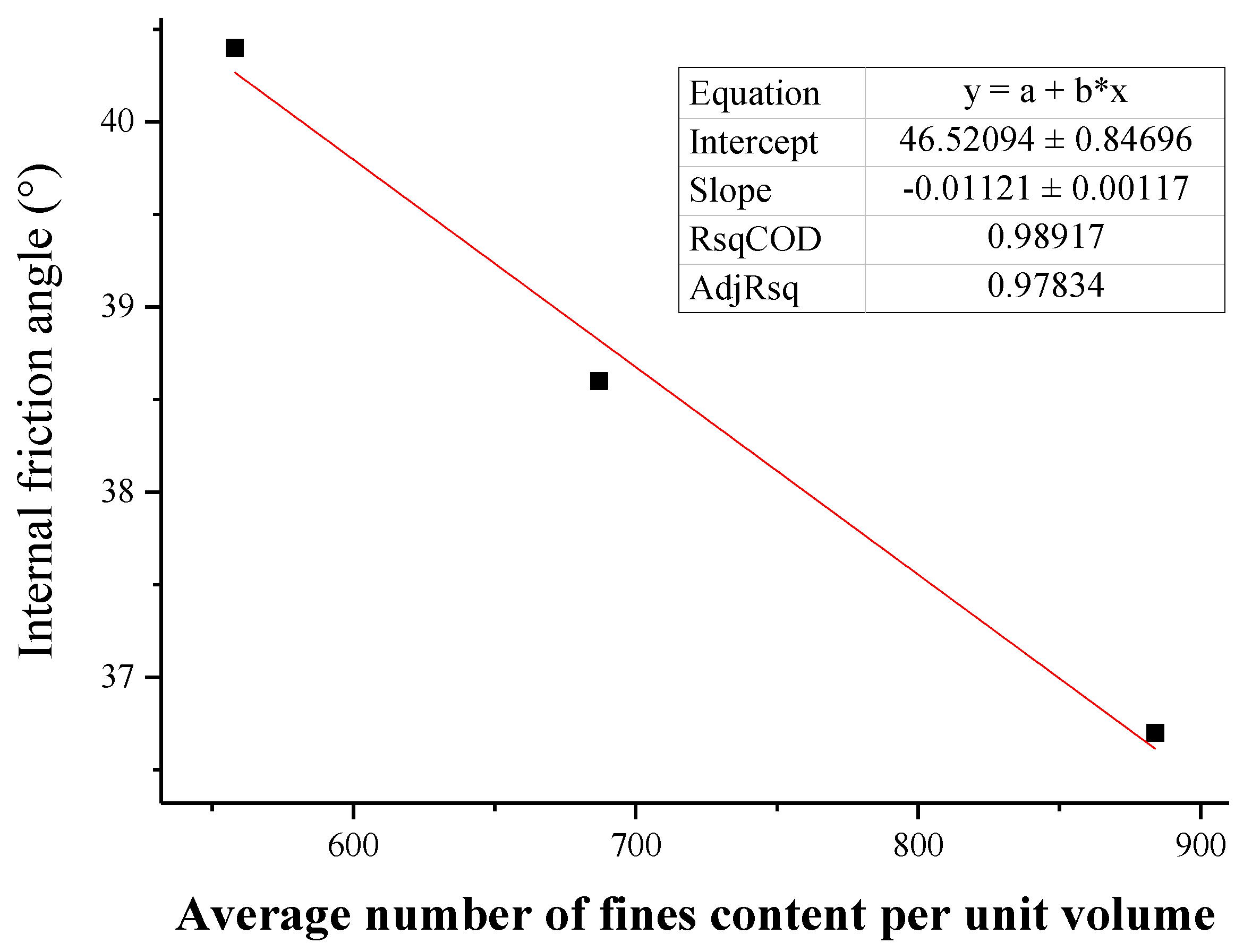
Figure 23.
Fitting curve of the fine particle content and internal friction angle per unit volume.
Figure 23.
Fitting curve of the fine particle content and internal friction angle per unit volume.
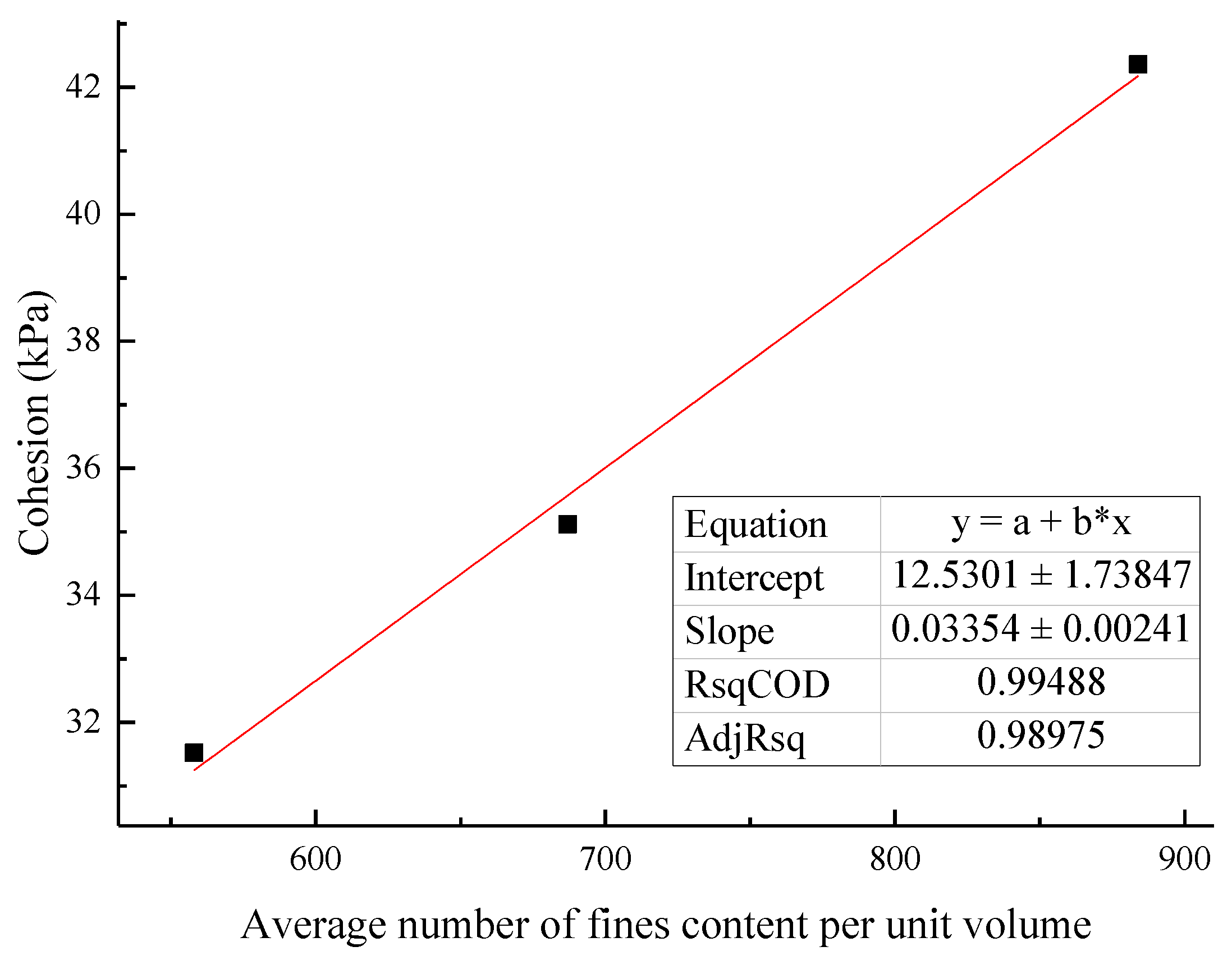
Figure 24.
Fitting curve of the fine particle content and cohesion per unit volume.
Figure 24.
Fitting curve of the fine particle content and cohesion per unit volume.
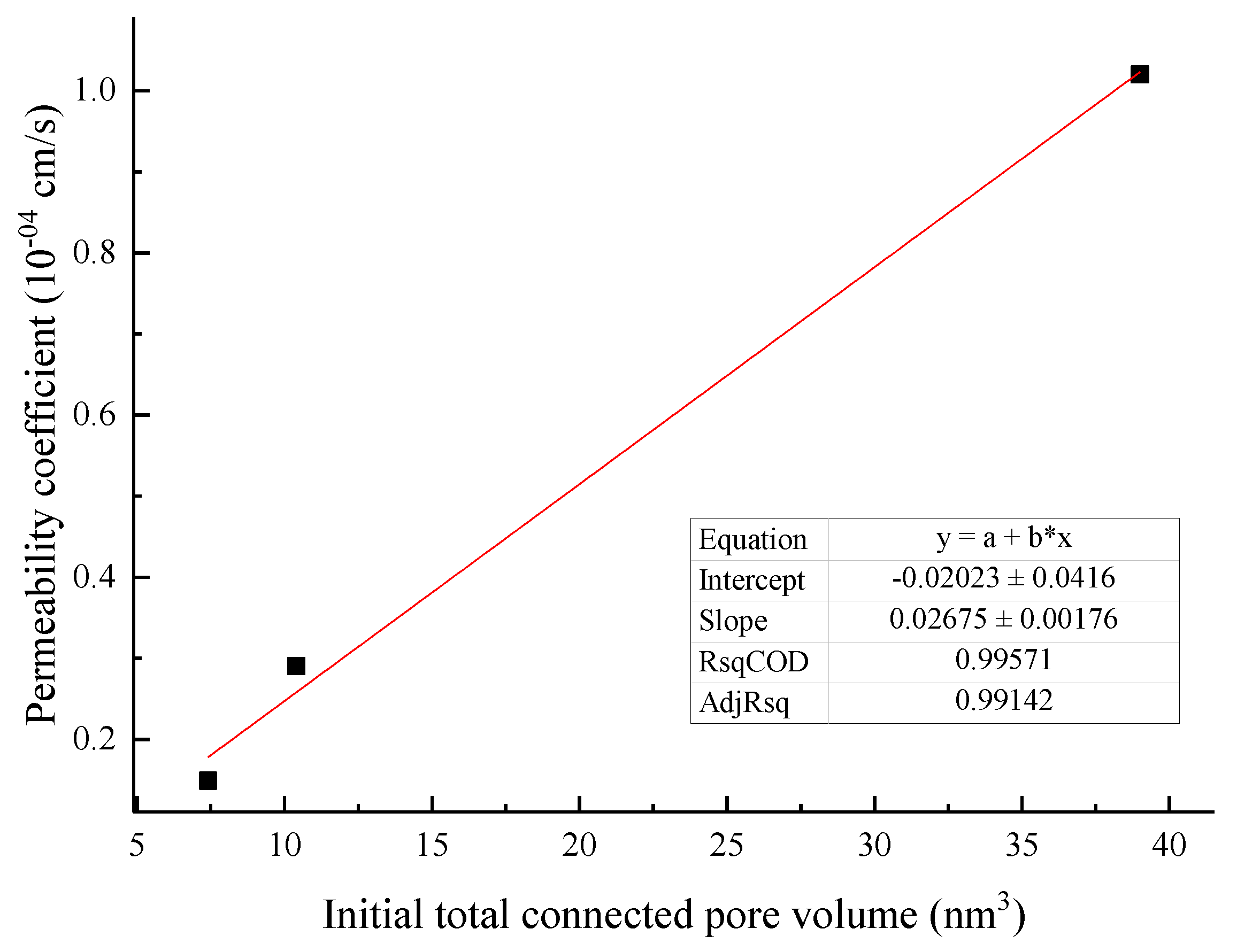
Figure 25.
Fitting curve of the connected pore volume and permeability coefficient.
Figure 25.
Fitting curve of the connected pore volume and permeability coefficient.
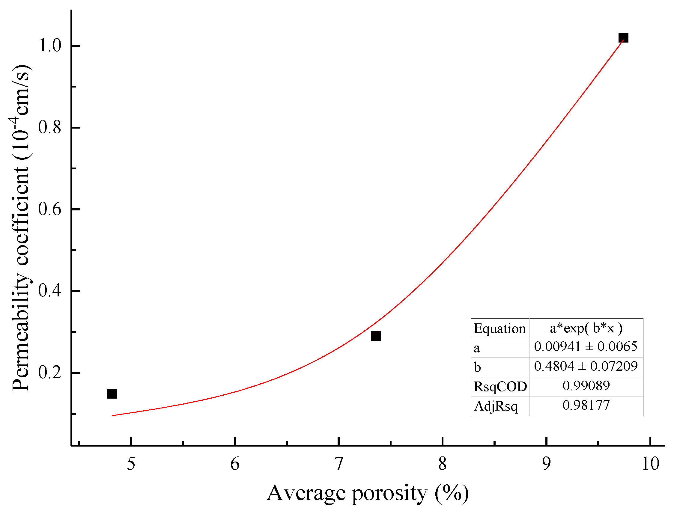
Figure 26.
The fitting curve of the average porosity and permeability coefficient.
Figure 26.
The fitting curve of the average porosity and permeability coefficient.
Table 1.
CT scan parameters.
Table 1.
CT scan parameters.
| Sample Name | Test Voltage/kV | Test Current/μA | Exposure Time/s | Resolution/μm | Pixel | X-ray Source to Sample Distance (sod)/mm | Distance from X-ray Source to Flat Panel Detector (sdd)/mm |
|---|
| Tailings sand sample | 140 | 70 | 0.42 | 6.16 | 1800 × 1800 × 1536 | 13.6 | 279.6 |
Table 2.
Head loading values at various levels.
Table 2.
Head loading values at various levels.
| Head Level | Loading Head Level/cm |
|---|
| 30% Fine Content | 50% Fine Content | 70% Fine Content |
|---|
| 1 | 29.0 | 32.0 | 48.0 |
| 2 | 37.0 | 43.0 | 52.0 |
| 3 | 39.0 | 46.0 | 56.0 |
| 4 | 42.0 | 51.0 | 58.0 |
Table 3.
Seepage velocity and permeability coefficient during the test.
Table 3.
Seepage velocity and permeability coefficient during the test.
| Fine Content | Head Level | Flow Rate
cm3/s | Permeability Coefficient
cm/s |
|---|
| 30% | 1 | 8.34 × 10⁻³ | 9.95 × 10⁻⁴ |
| 2 | 1.23 × 10⁻² | 1.14 × 10⁻³ |
| 3 | 2.78 × 10⁻² | 2.45 × 10⁻³ |
| 4 | 8.34 × 10⁻² | 6.52 × 10⁻³ |
| 50% | 1 | 7.59 × 10⁻³ | 8.18 × 10⁻⁴ |
| 2 | 1.30 × 10⁻² | 1.04 × 10⁻³ |
| 3 | 2.98 × 10⁻² | 2.23 × 10⁻³ |
| 4 | 5.96 × 10⁻² | 4.01 × 10⁻³ |
| 70% | 1 | 6.95 × 10⁻³ | 6.30 × 10⁻⁴ |
| 2 | 1.30 × 10⁻² | 8.60 × 10⁻⁴ |
| 3 | 1.67 × 10⁻² | 1.02 × 10⁻³ |
| 4 | 6.95 × 10⁻² | 3.84 × 10⁻³ |
Table 4.
Statistics of the number of pores in the seepage process with the 30% fine content.
Table 4.
Statistics of the number of pores in the seepage process with the 30% fine content.
| Head Level | Pore Size D/µm | Total Number of Pores | Total Connected Pore Volume (µm3) |
|---|
| 0–10 | 10–20 | 20–40 | 40–80 | >80 |
|---|
| 1 | 210,450 | 129,578 | 35,057 | 9092 | 4557 | 388,734 | 3.9 × 10¹⁰ |
| 2 | 166,833 | 138,197 | 40,293 | 9347 | 3983 | 358,653 | 6.05 × 10¹⁰ |
| 3 | 133,557 | 156,602 | 41,543 | 10,553 | 4702 | 346,957 | 6.5 × 10¹⁰ |
| 4 | 81,410 | 140,923 | 44,661 | 24,151 | 6170 | 297,315 | 8.34 × 10¹⁰ |
Table 5.
Statistics of the number of pores in the seepage process with the 50% fine content.
Table 5.
Statistics of the number of pores in the seepage process with the 50% fine content.
| Head Level | Pore Size D/µm | Total Number of Pores | Total Connected Pore Volume (µm3) |
|---|
| 0–10 | 10–20 | 20–40 | 40–80 | >80 |
|---|
| 1 | 126,404 | 87,362 | 44,256 | 23,020 | 9373 | 290,415 | 1.04 × 10¹⁰ |
| 2 | 151,873 | 103,059 | 31,162 | 22,938 | 8224 | 317,256 | 2.32 × 10¹⁰ |
| 3 | 142,467 | 97,344 | 41,445 | 19,447 | 6450 | 307,153 | 2.75 × 10¹⁰ |
| 4 | 283,942 | 184,156 | 55,797 | 18,723 | 5370 | 547,988 | 3.47 × 10¹⁰ |
Table 6.
Statistics of the number of pores in the seepage process with the 70% fine content.
Table 6.
Statistics of the number of pores in the seepage process with the 70% fine content.
| Head Level | Pore Size D/µm | Total Number of Pores | Total Connected Pore Volume (µm3) |
|---|
| 0–10 | 10–20 | 20–40 | 40–80 | >80 |
|---|
| 1 | 144,629 | 92,459 | 51,268 | 27,397 | 8370 | 324,123 | 7.41 × 10⁹ |
| 2 | 121,473 | 79,449 | 28,819 | 12,602 | 3745 | 246,088 | 1.43 × 10¹⁰ |
| 3 | 239,642 | 169,238 | 62,833 | 20,485 | 2605 | 494,803 | 4.8 × 10¹⁰ |
| 4 | 555,965 | 321,095 | 83,504 | 19,136 | 2809 | 982,509 | 5.74 × 10¹⁰ |
Table 7.
Variation in the number of fine particles percolated with the 30% fine content (0–10 µm).
Table 7.
Variation in the number of fine particles percolated with the 30% fine content (0–10 µm).
| Head Level | Layers | Total Number of Particles |
|---|
| 0–200 Layers | 200–400 Layers | 400–600 Layers | 600–800 Layers | 800–1000 Layers | 0–10 μm |
|---|
| 1 | 26,653 | 20,791 | 17,301 | 17,441 | 18,944 | 101,130 |
| 2 | 19,751 | 14,573 | 14,862 | 15,978 | 19,242 | 84,406 |
| 3 | 16,894 | 14,363 | 13,917 | 13,750 | 16,062 | 74,986 |
| 4 | 18,444 | 15,048 | 14,558 | 14,469 | 12,000 | 74,519 |
Table 8.
Variation in the number of fine particles percolated with the 30% fine content (10–20 µm).
Table 8.
Variation in the number of fine particles percolated with the 30% fine content (10–20 µm).
| Head Level | Layers | Total Number of Particles |
|---|
| 0–200 Layers | 200–400 Layers | 400–600 Layers | 600–800 Layers | 800–1000 Layers | 10–20 μm |
|---|
| 1 | 19,241 | 16,522 | 14,149 | 13,905 | 14,608 | 78,425 |
| 2 | 15,282 | 12,091 | 12,460 | 13,044 | 16,546 | 69,423 |
| 3 | 12,337 | 10,511 | 11,703 | 10,406 | 14,108 | 59,065 |
| 4 | 14,183 | 10,871 | 9400 | 10,753 | 11,156 | 56,363 |
Table 9.
Variation in the number of fine particles percolated with the 30% fine content (20–40 µm).
Table 9.
Variation in the number of fine particles percolated with the 30% fine content (20–40 µm).
| Head Level | Layers | Total Number of Particles |
|---|
| 0–200 Layers | 200–400 Layers | 400–600 Layers | 600–800 Layers | 800–1000 Layers | 20–40 μm |
|---|
| 1 | 10,450 | 10,572 | 10,384 | 10,157 | 10,312 | 51,875 |
| 2 | 10,248 | 9187 | 9322 | 9704 | 10,299 | 48,760 |
| 3 | 7881 | 7220 | 7186 | 7160 | 9973 | 39,420 |
| 4 | 7423 | 7080 | 7315 | 7237 | 8605 | 37,660 |
Table 10.
Variation in the number of fine particles percolated with the 30% fine content (40–75 µm).
Table 10.
Variation in the number of fine particles percolated with the 30% fine content (40–75 µm).
| Head Level | Layers | Total Number of Particles |
|---|
| 0–200 Layers | 200–400 Layers | 400–600 Layers | 600–800 Layers | 800–1000 Layers | 40–75 μm |
|---|
| 1 | 7721 | 7394 | 7518 | 7758 | 8038 | 38,429 |
| 2 | 7472 | 7144 | 7095 | 7247 | 8036 | 36,994 |
| 3 | 6086 | 5661 | 5388 | 5582 | 6844 | 29,561 |
| 4 | 5591 | 5814 | 6387 | 6161 | 6644 | 30,597 |
Table 11.
Variation in the number of fine particles percolated with the 50% fine particle content (0–10 µm).
Table 11.
Variation in the number of fine particles percolated with the 50% fine particle content (0–10 µm).
| Head Level | Layers | Total Number of Particles |
|---|
| 0–200 Layers | 200–400 Layers | 400–600 Layers | 600–800 Layers | 800–1000 Layers | 0–10 µm |
|---|
| 1 | 23,766 | 18,299 | 17,785 | 16,910 | 16,568 | 93,328 |
| 2 | 26,602 | 19,188 | 18,753 | 19,365 | 16,355 | 100,263 |
| 3 | 18,741 | 14,446 | 16,426 | 16,607 | 15,548 | 81,768 |
| 4 | 42,318 | 28,355 | 19,772 | 24,064 | 23,177 | 137,686 |
Table 12.
Variation in the number of fine particles percolated with the 50% fine particle content (10–20 µm).
Table 12.
Variation in the number of fine particles percolated with the 50% fine particle content (10–20 µm).
| Head Level | Layers | Total Number of Particles |
|---|
| 0–200 Layers | 200–400 Layers | 400–600 Layers | 600–800 Layers | 800–1000 Layers | 10–20 µm |
|---|
| 1 | 33,729 | 18,744 | 19,050 | 18,225 | 17,541 | 107,289 |
| 2 | 24,766 | 19,084 | 19,974 | 19,998 | 16,777 | 100,599 |
| 3 | 18,999 | 15,798 | 17,927 | 17,105 | 15,843 | 85,672 |
| 4 | 35,974 | 27,324 | 22,419 | 25,302 | 24,038 | 135,057 |
Table 13.
Variation in the number of fine particles percolated with the 50% fine particle content (20–40 µm).
Table 13.
Variation in the number of fine particles percolated with the 50% fine particle content (20–40 µm).
| Head Level | Layers | Total Number of Particles |
|---|
| 0–200 Layers | 200–400 Layers | 400–600 Layers | 600–800 Layers | 800–1000 Layers | 20–40 μm |
|---|
| 1 | 18,156 | 15,488 | 16,652 | 15,824 | 15,339 | 81,459 |
| 2 | 17,645 | 15,627 | 16,806 | 16,350 | 15,042 | 81,470 |
| 3 | 15,878 | 13,677 | 15,650 | 14,216 | 13,299 | 72,720 |
| 4 | 19,534 | 17,989 | 18,778 | 19,091 | 18,482 | 93,874 |
Table 14.
Variation in the number of fine particles percolated with the 50% fine particle content (40–75 µm).
Table 14.
Variation in the number of fine particles percolated with the 50% fine particle content (40–75 µm).
| Head Level | Layers | Total Number of Particles |
|---|
| 0–200 Layers | 200–400 Layers | 400–600 Layers | 600–800 Layers | 800–1000 Layers | 40–75 μm |
|---|
| 1 | 9920 | 9387 | 10,290 | 10,190 | 10,485 | 50,272 |
| 2 | 9221 | 8956 | 9944 | 10,209 | 10,179 | 48,509 |
| 3 | 9459 | 8609 | 9782 | 9287 | 8721 | 45,858 |
| 4 | 6976 | 7723 | 9674 | 10,053 | 9544 | 43,970 |
Table 15.
Variation in the number of fine particles percolated with the 70% fine particle content (0–10 µm).
Table 15.
Variation in the number of fine particles percolated with the 70% fine particle content (0–10 µm).
| Head Level | Layers | Total Number of Particles |
|---|
| 0–200 Layers | 200–400 Layers | 400–600 Layers | 600–800 Layers | 800–1000 Layers | 0–10 µm |
|---|
| 1 | 87,828 | 391 | 766 | 40,270 | 32,733 | 161,988 |
| 2 | 19,479 | 22,673 | 19,724 | 20,699 | 15,542 | 98,117 |
| 3 | 34,604 | 26,022 | 24,874 | 24,237 | 23,683 | 133,420 |
| 4 | 45,777 | 27,944 | 22,124 | 21,434 | 22,105 | 139,384 |
Table 16.
Variation in the number of fine particles percolated with the 70% fine particle content (10–20 µm).
Table 16.
Variation in the number of fine particles percolated with the 70% fine particle content (10–20 µm).
| Head Level | Layers | Total Number of Particles |
|---|
| 0–200 Layers | 200–400 Layers | 400–600 Layers | 600–800 Layers | 800–1000 Layers | 10–20 μm |
|---|
| 1 | 55,980 | 841 | 1118 | 34,591 | 29,263 | 121,793 |
| 2 | 16,891 | 20,360 | 17,716 | 18,240 | 13,863 | 87,070 |
| 3 | 32,021 | 26,572 | 25,585 | 26,746 | 23,308 | 134,232 |
| 4 | 39,505 | 28,175 | 23,089 | 22,083 | 21,968 | 134,820 |
Table 17.
Variation in the number of fine particles percolated with the 70% fine particle content (20-40 µm).
Table 17.
Variation in the number of fine particles percolated with the 70% fine particle content (20-40 µm).
| Head Level | Layers | Total Number of Particles |
|---|
| 0–200 Layers | 200–400 Layers | 400–600 Layers | 600–800 Layers | 800–1000 Layers | 20–40 μm |
|---|
| 1 | 23,315 | 5911 | 3267 | 23,898 | 21,525 | 77,916 |
| 2 | 12,441 | 15,808 | 13,941 | 14,219 | 11,125 | 67,534 |
| 3 | 23,148 | 21,702 | 20,354 | 22,096 | 18,821 | 106,121 |
| 4 | 26,506 | 23,883 | 20,851 | 19,905 | 18,711 | 109,856 |
Table 18.
Variation in the number of fine particles percolated with the 70% fine particle content (40–75 µm).
Table 18.
Variation in the number of fine particles percolated with the 70% fine particle content (40–75 µm).
| Head Level | Layers | Total Number of Particles |
|---|
| 0–200 Layers | 200–400 Layers | 400–600 Layers | 600–800 Layers | 800–1000 Layers | 40–75 μm |
|---|
| 1 | 7115 | 8975 | 6980 | 11,679 | 11,576 | 46,325 |
| 2 | 7160 | 9582 | 8743 | 8640 | 6796 | 40,921 |
| 3 | 11,566 | 11,140 | 10,648 | 11,728 | 10,212 | 55,294 |
| 4 | 12,209 | 12,674 | 11,978 | 11,141 | 10,387 | 58,389 |
Table 19.
Fine particle content change during seepage (0–10 µm).
Table 19.
Fine particle content change during seepage (0–10 µm).
| Head Level | 30% Fine Content | 50% Fine Content | 70% Fine Content |
|---|
| 1 | 101,130 | 93,328 | 161,988 |
| 2 | 84,406 | 100,263 | 98,117 |
| 3 | 74,986 | 81,768 | 133,420 |
| 4 | 74,519 | 137,686 | 139,384 |
Table 20.
Fine particle content change during seepage (10–20 µm).
Table 20.
Fine particle content change during seepage (10–20 µm).
| Head Level | 30% Fine Content | 50% Fine Content | 70% Fine Content |
|---|
| 1 | 78,425 | 107,289 | 161,988 |
| 2 | 69,423 | 100,599 | 98,117 |
| 3 | 59,065 | 85,672 | 133,420 |
| 4 | 56,363 | 135,057 | 139,384 |
Table 21.
Fine particle content change during seepage (20–40 µm).
Table 21.
Fine particle content change during seepage (20–40 µm).
| Head Level | 30% Fine Content | 50% Fine Content | 70% Fine Content |
|---|
| 1 | 51875 | 81459 | 77916 |
| 2 | 48760 | 81470 | 67534 |
| 3 | 39420 | 72720 | 106121 |
| 4 | 37,660 | 93,874 | 109,856 |
Table 22.
Fine particle content change during seepage (40–75 µm).
Table 22.
Fine particle content change during seepage (40–75 µm).
| Head Level | 30% Fine Content | 50% Fine Content | 70% Fine Content |
|---|
| 1 | 38,429 | 50,272 | 46,325 |
| 2 | 36,994 | 48,509 | 40,921 |
| 3 | 29,561 | 45,858 | 55,294 |
| 4 | 30,597 | 43,970 | 58,389 |
Table 23.
Fine particle content change during seepage (0–75 µm).
Table 23.
Fine particle content change during seepage (0–75 µm).
| Head Level | 30% Fine Content | 50% Fine Content | 70% Fine Content |
|---|
| 1 | 269,859 | 332,347 | 408,023 |
| 2 | 239,583 | 330,842 | 293,643 |
| 3 | 203,031 | 286,018 | 429,067 |
| 4 | 199,139 | 410,587 | 442,449 |
Table 24.
Macro- and mesofactor comparison table.
Table 24.
Macro- and mesofactor comparison table.
| Fine Content | Fine Content Total Number of Particles | Average Number of Fine Content Per Unit Volume | Average Porosity
% | Total Volume of Initial Connected Pores | Permeability Coefficient
(cm·s−1) | Internal Friction Angle
ϕ/° | Cohesion
c/kPa |
|---|
| 30% | 269,859 | 558 | 9.74342101 | 3.90 × 10¹⁰ | 1.02 × 10⁻⁴ | 40.4 | 31.52 |
| 50% | 332,347 | 687 | 7.35860292 | 1.04 × 10¹⁰ | 2.90 × 10⁻⁵ | 38.6 | 35.12 |
| 70% | 408,023 | 884 | 4.81893178 | 7.41 × 10⁹ | 1.49 × 10⁻⁵ | 36.7 | 42.36 |


