Visual Appearance of Nanocrystal-Based Luminescent Solar Concentrators


Abstract
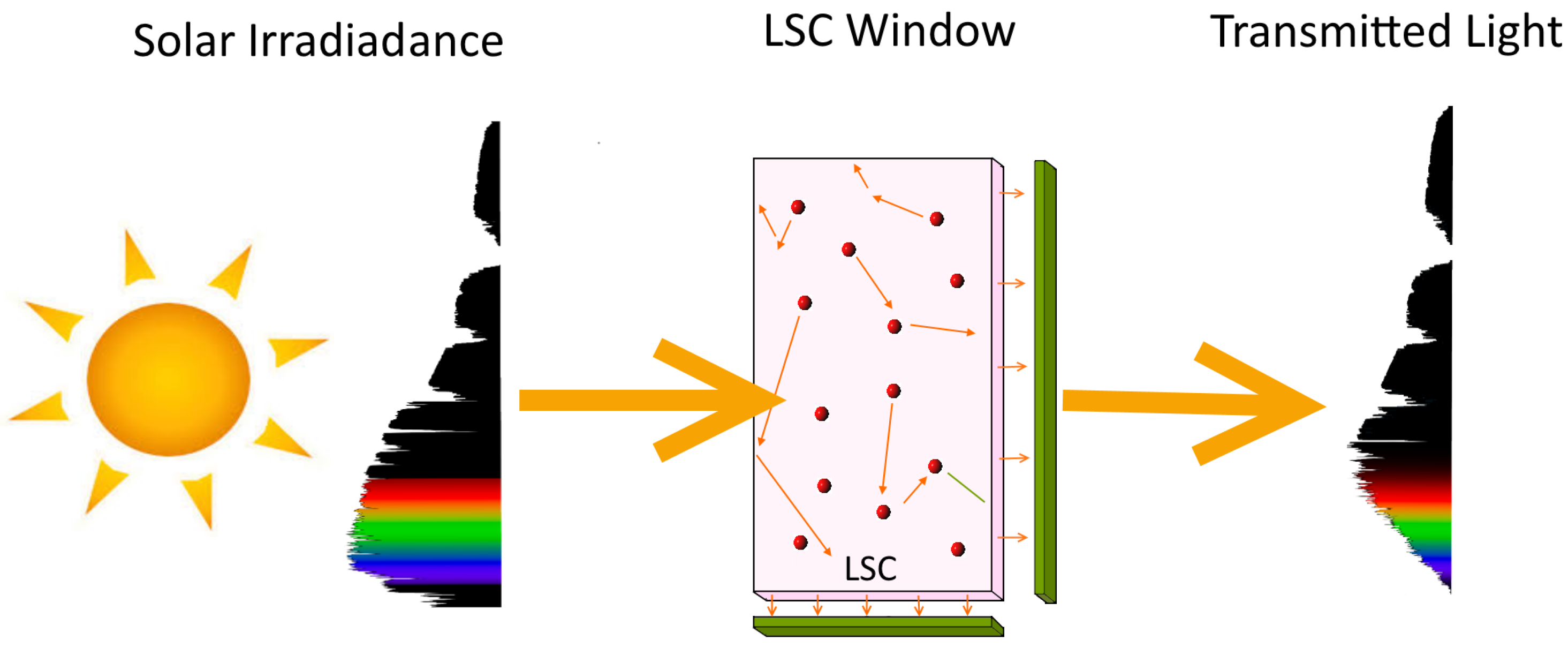
:1. Introduction
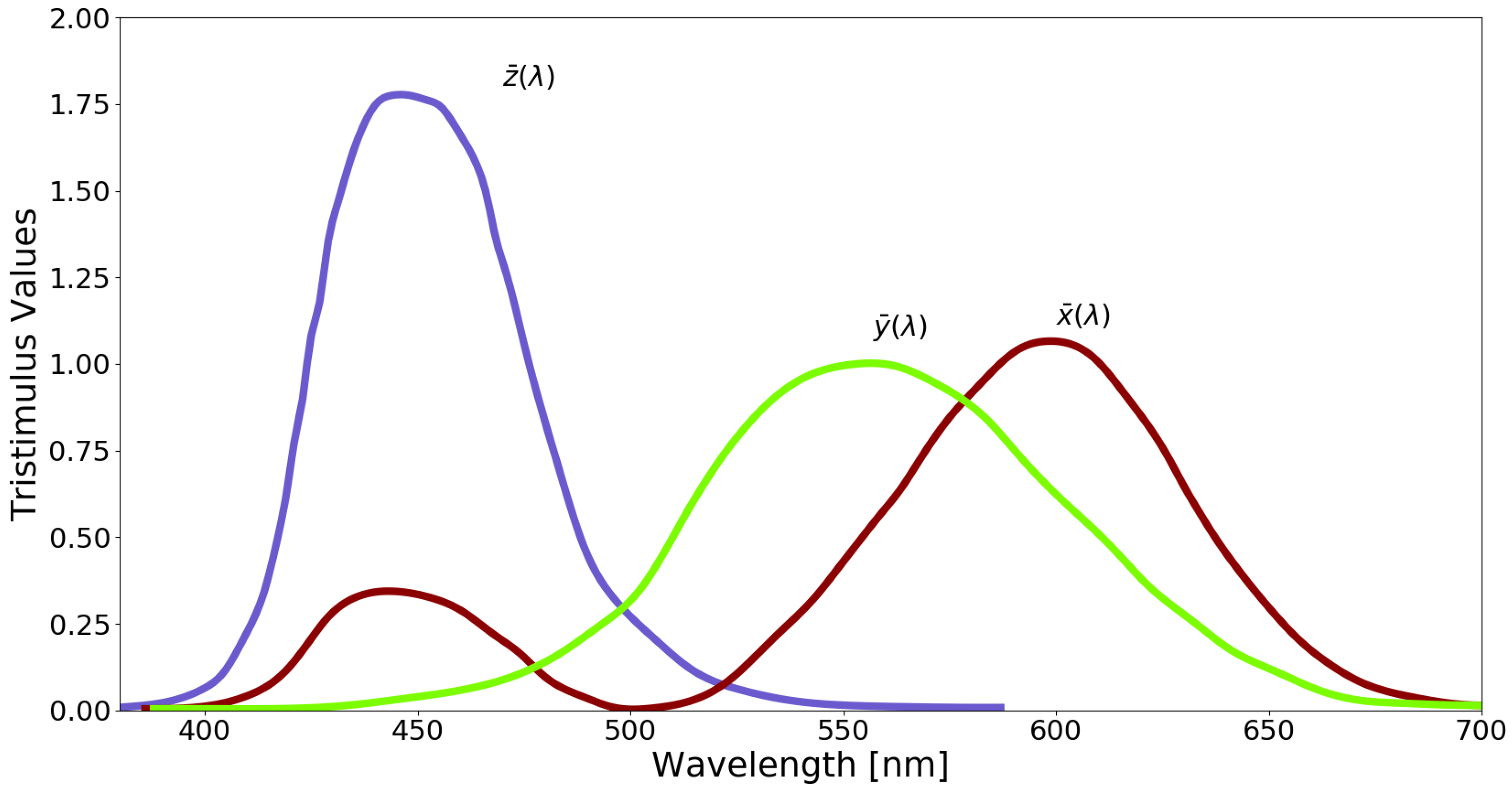
2. Colorimetry
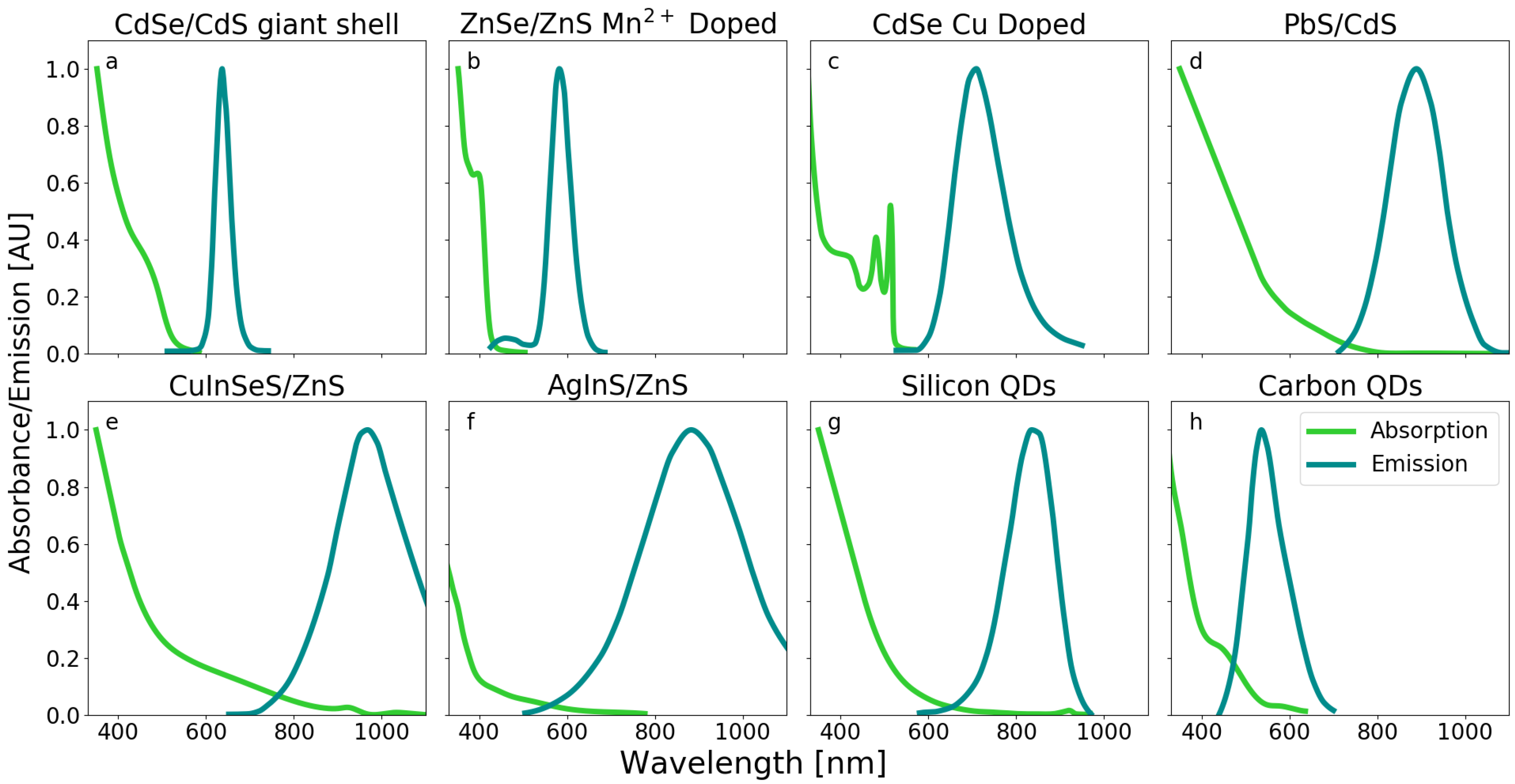
3. Luminophores
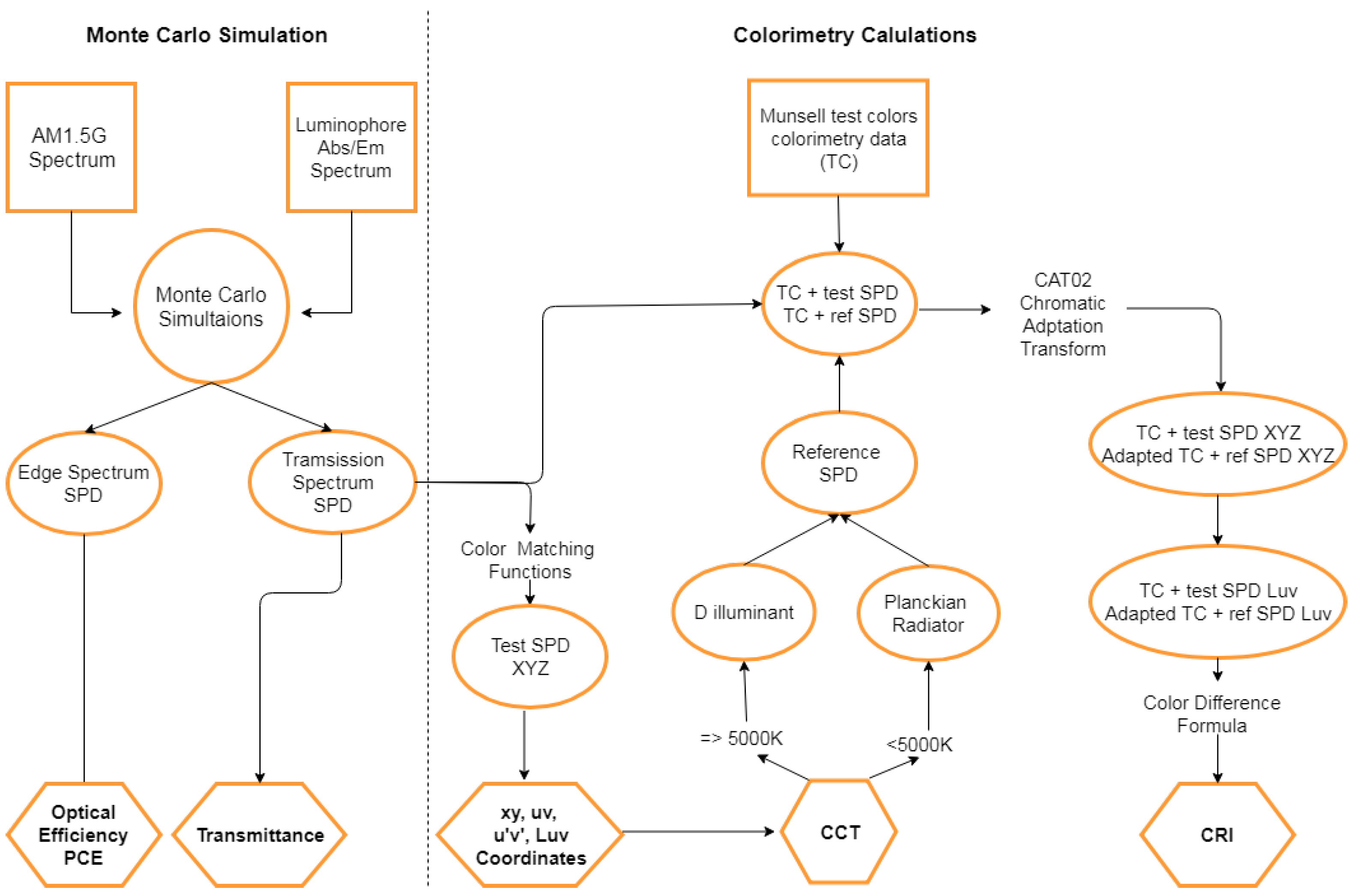
4. Method
4.1. Overview
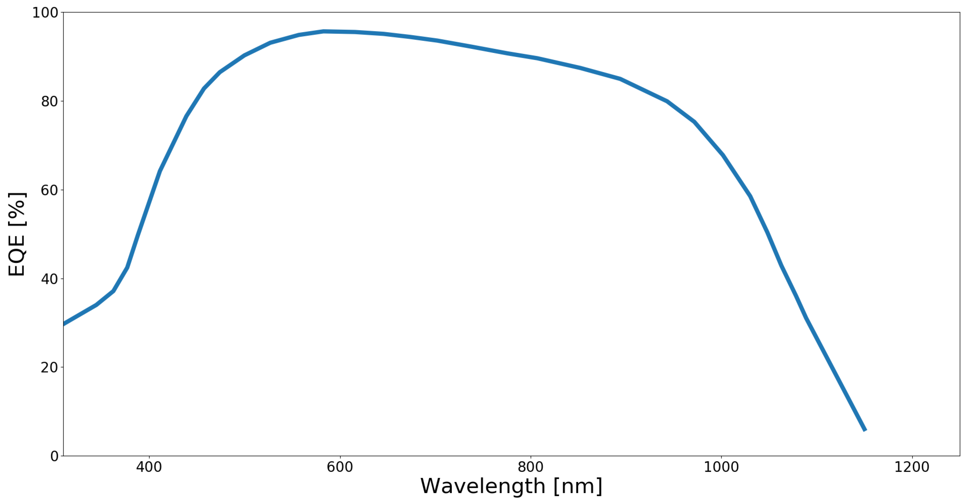
4.2. Monte-Carlo Simulations
4.3. Colorimetric Performance
5. Results
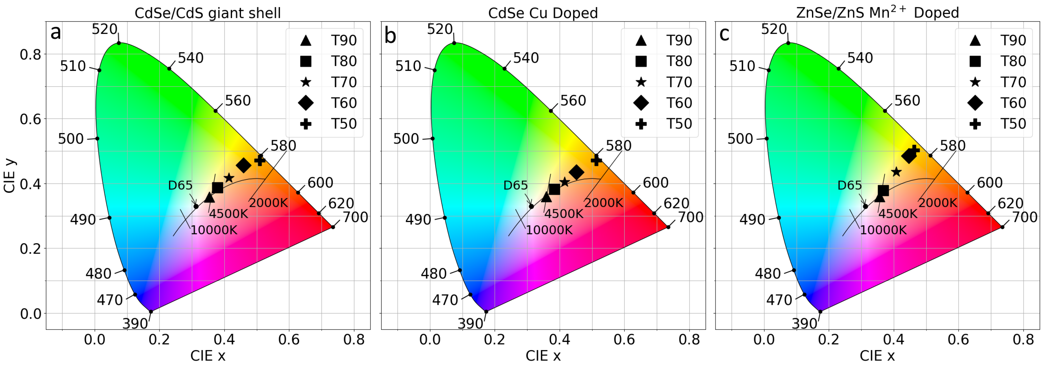
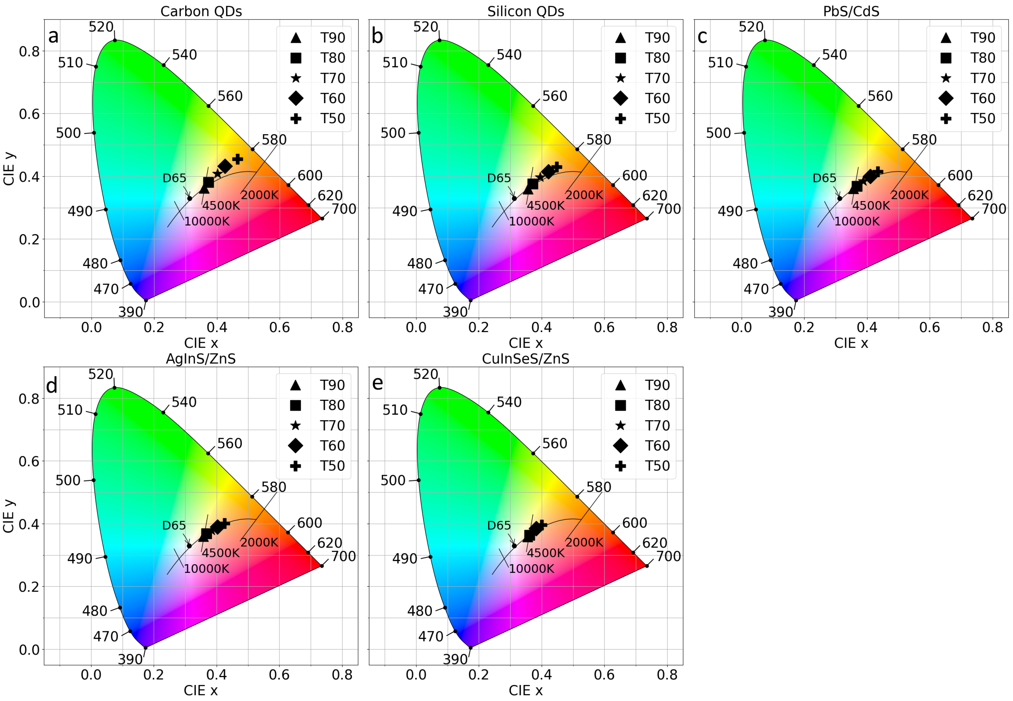
5.1. Colorimetry Assessment
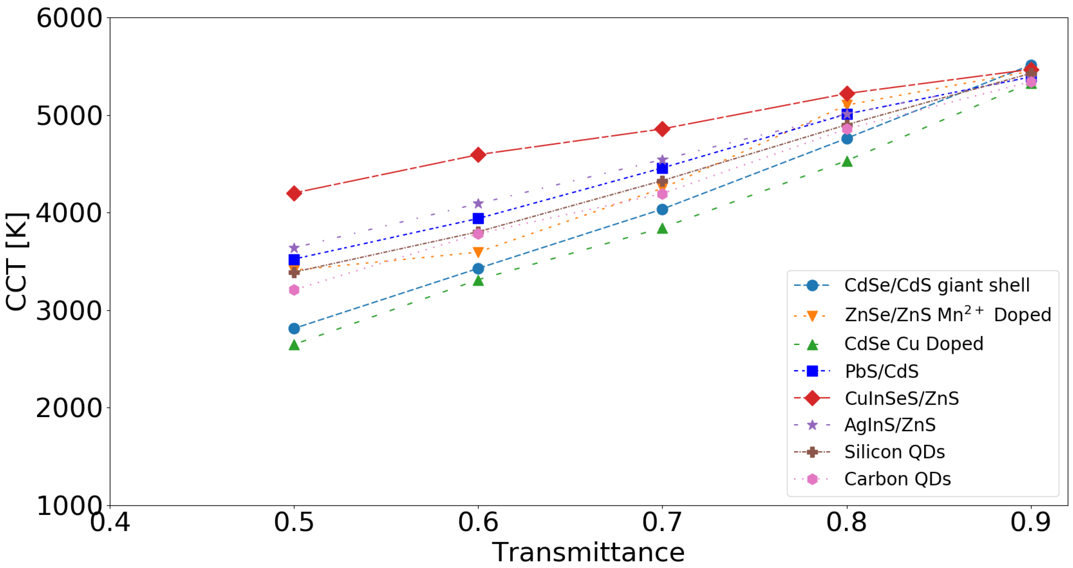
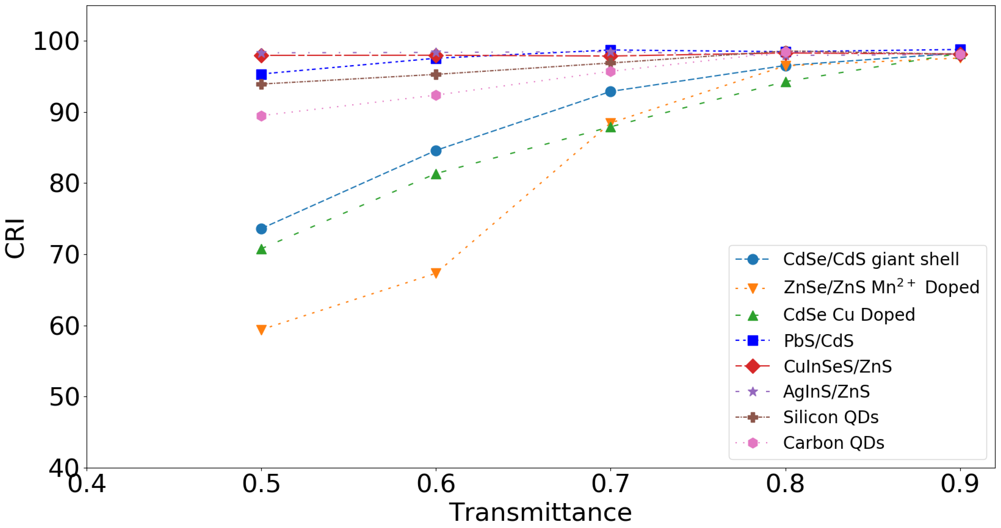
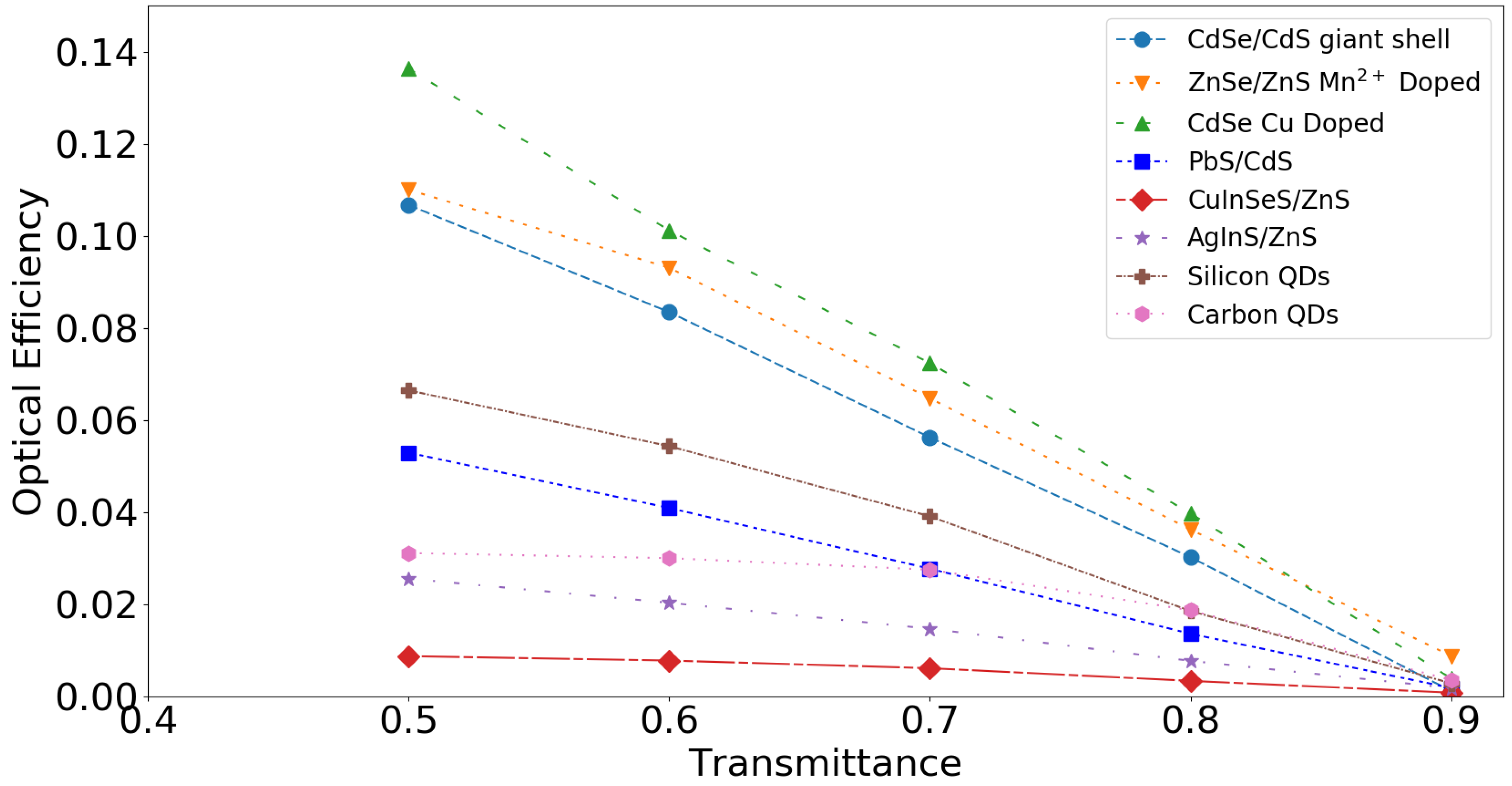
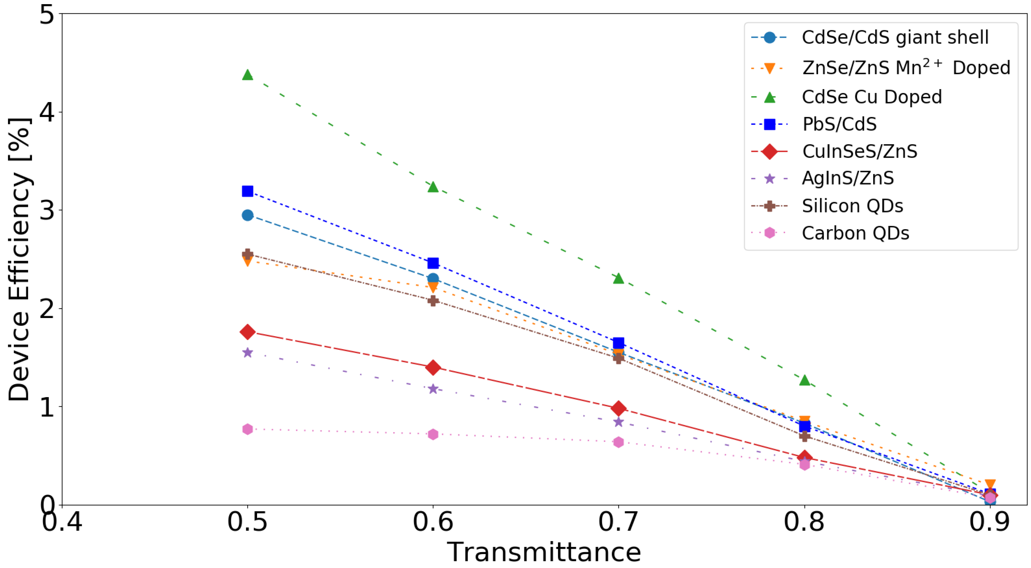
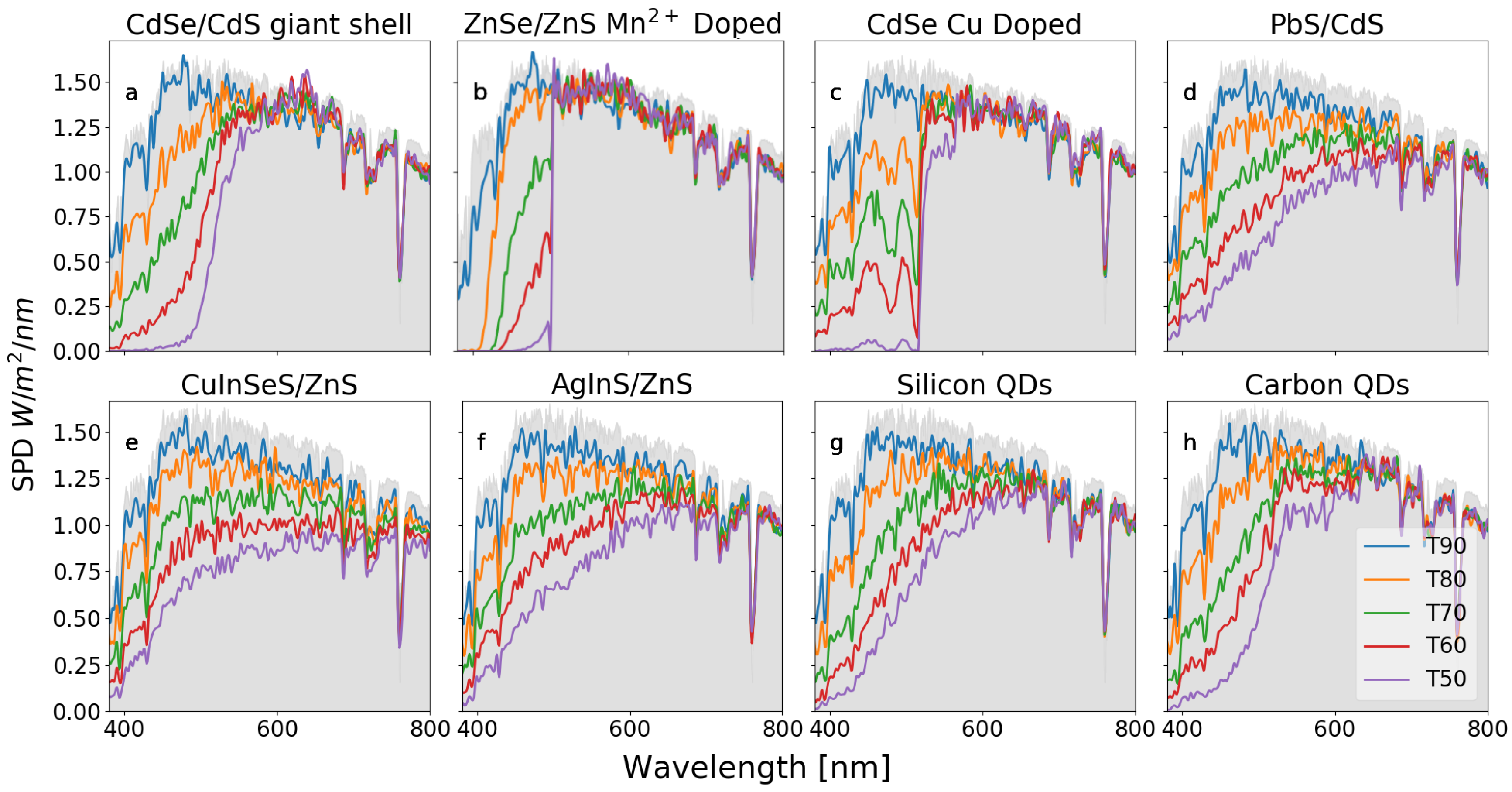
5.2. Performance Analysis
6. Conclusions
Author Contributions
Funding
Conflicts of Interest
References
- International Energy Agency. Transition to Sustainable Buildings: Strategies and Opportunities to 2050; OECD: Paris, France, 2013.
- International Energy Agency. Energy Technology Perspectives 2017: Catalysing Energy Technology Transformations; OECD: Paris, France, 2017.
- Parliament, E.; The Council. Council Regulation No 1177/2010. Off. J. Eur. Union 2010, 334, 1–16. [Google Scholar]
- Reinders, A.; Verlinden, P.; van Sark, W.; Freundlich, A. Photovoltaic Solar Energy; John Wiley & Sons, Ltd.: Chichester, UK, 2016. [Google Scholar]
- International Energy Agency. Market Report Series: Renewables 2018; IEA Publications: Paris, France, 2018.
- Mayer, J.N. Current and Future Cost of Photovoltaics. Long-Term Scenarios for Market Development, System Prices and LCOE of Utility-Scale PV Systems. Study on Behalf of Agora Energiewende; Fraunhofer ISE: Freiburg, Germany, 2015. [Google Scholar]
- Moraitis, P.; Kausika, B.; Nortier, N.; van Sark, W. Urban Environment and Solar PV Performance: The Case of the Netherlands. Energies 2018, 11, 1333. [Google Scholar] [CrossRef]
- Debije, M.G.; Verbunt, P.P.C. Thirty Years of Luminescent Solar Concentrator Research: Solar Energy for the Built Environment. Adv. Energy Mater. 2011, 2, 12–35. [Google Scholar] [CrossRef]
- Meinardi, F.; Bruni, F.; Brovelli, S. Luminescent solar concentrators for building-integrated photovoltaics. Nat. Rev. Mater. 2017, 2, 17072. [Google Scholar] [CrossRef]
- Van Sark, W.G. Luminescent solar concentrators—A low cost photovoltaics alternative. Renew. Energy 2013, 49, 207–210. [Google Scholar] [CrossRef]
- Debije, M.G.; Rajkumar, V.A. Direct versus indirect illumination of a prototype luminescent solar concentrator. Sol. Energy 2015, 122, 334–340. [Google Scholar] [CrossRef]
- Moraitis, P.; Schropp, R.; van Sark, W. Nanoparticles for Luminescent Solar Concentrators—A review. Opt. Mater. 2018, 84, 636–645. [Google Scholar] [CrossRef]
- Traverse, C.J.; Pandey, R.; Barr, M.C.; Lunt, R.R. Emergence of highly transparent photovoltaics for distributed applications. Nat. Energy 2017, 2, 849–860. [Google Scholar] [CrossRef]
- Debije, M.G. Solar Energy Collectors with Tunable Transmission. Adv. Funct. Mater. 2010, 20, 1498–1502. [Google Scholar] [CrossRef]
- Corrado, C.; Leow, S.W.; Osborn, M.; Carbone, I.; Hellier, K.; Short, M.; Alers, G.; Carter, S.A. Power generation study of luminescent solar concentrator greenhouse. J. Renew. Sustain. Energy 2016, 8, 043502. [Google Scholar] [CrossRef]
- Kanellis, M.; de Jong, M.M.; Slooff, L.; Debije, M.G. The solar noise barrier project: 1. Effect of incident light orientation on the performance of a large-scale luminescent solar concentrator noise barrier. Renew. Energy 2017, 103, 647–652. [Google Scholar] [CrossRef]
- Van Sark, W.; Moraitis, P.; Aalberts, C.; Drent, M.; Grasso, T.; Ortije, Y.L.; Visschers, M.; Westra, M.; Plas, R.; Planje, W. The Electric Mondrian as a Luminescent Solar Concentrator Demonstrator Case Study. Sol. RRL 2017, 1, 1600015. [Google Scholar] [CrossRef]
- Reinders, A.H.M.E.; de la Gree, G.D.; Papadopoulos, A.; Rosemann, A.; Debije, M.G.; Cox, M.; Krumer, Z. Leaf roof Designing luminescent solar concentrating PV roof tiles. In Proceedings of the 2016 IEEE 43rd Photovoltaic Specialists Conference (PVSC), Portland, OR, USA, 5–10 July 2016. [Google Scholar] [CrossRef]
- Aste, N.; Buzzetti, M.; Pero, C.D.; Fusco, R.; Testa, D.; Leonforte, F. Visual Performance of Yellow, Orange and Red LSCs Integrated in a Smart Window. Energy Proced. 2017, 105, 967–972. [Google Scholar] [CrossRef]
- Aste, N.; Tagliabue, L.C.; Palladino, P.; Testa, D. Integration of a luminescent solar concentrator: Effects on daylight, correlated color temperature, illuminance level and color rendering index. Sol. Energy 2015, 114, 174–182. [Google Scholar] [CrossRef]
- Lynn, N.; Mohanty, L.; Wittkopf, S. Color rendering properties of semi-transparent thin-film PV modules. Build. Environ. 2012, 54, 148–158. [Google Scholar] [CrossRef]
- Bellia, L.; Bisegna, F.; Spada, G. Lighting in indoor environments: Visual and non-visual effects of light sources with different spectral power distributions. Build. Environ. 2011, 46, 1984–1992. [Google Scholar] [CrossRef]
- Knez, I.; Kers, C. Effects of Indoor Lighting, Gender, and Age on Mood and Cognitive Performance. Environ. Behav. 2000, 32, 817–831. [Google Scholar] [CrossRef]
- Partonen, T.; Lönnqvist, J. Bright light improves vitality and alleviates distress in healthy people. J. Affect. Disord. 2000, 57, 55–61. [Google Scholar] [CrossRef]
- Dangol, R.; Islam, M.; LiSc, M.H.; Bhusal, P.; Puolakka, M.; Halonen, L. Subjective preferences and colour quality metrics of LED light sources. Light. Res. Technol. 2013, 45, 666–688. [Google Scholar] [CrossRef]
- Vossen, F.M.; Aarts, M.P.; Debije, M.G. Visual performance of red luminescent solar concentrating windows in an office environment. Energy Build. 2016, 113, 123–132. [Google Scholar] [CrossRef]
- Hunt, R.W.G.; Pointer, M.R. Measuring Colour; John Wiley & Sons Inc.: Chichester, UK, 2011. [Google Scholar]
- Gunde, M.K.; Krašovec, U.O.; Platzer, W.J. Color rendering properties of interior lighting influenced by a switchable window. J. Opt. Soc. Am. A 2005, 22, 416. [Google Scholar] [CrossRef]
- De L’Eclairage, C.I. CIE 013.3-1995: Method of Measuring and Specifying Colour Rendering Properties of Light Sources; Commission Internationale de L’Eclairage: Vienna, Austria, 1995. [Google Scholar]
- Karlicek, R.; Sun, C.-C.; Zissis, G.; Ma, R. Handbook of Advanced Lighting Technology. 2 Volumes; Springer-Verlag GmbH: Berlin, Germany, 2017. [Google Scholar]
- De Mello Donegá, C. Synthesis and properties of colloidal heteronanocrystals. Chem. Soc. Rev. 2011, 40, 1512–1546. [Google Scholar] [CrossRef] [PubMed]
- Chen, Y.; Vela, J.; Htoon, H.; Casson, J.L.; Werder, D.J.; Bussian, D.A.; Klimov, V.I.; Hollingsworth, J.A. “Giant” Multishell CdSe Nanocrystal Quantum Dots with Suppressed Blinking. J. Am. Chem. Soc. 2008, 130, 5026–5027. [Google Scholar] [CrossRef]
- Meinardi, F.; Colombo, A.; Velizhanin, K.A.; Simonutti, R.; Lorenzon, M.; Beverina, L.; Viswanatha, R.; Klimov, V.I.; Brovelli, S. Large-area luminescent solar concentrators based on `Stokes-shift-engineered’ nanocrystals in a mass-polymerized PMMA matrix. Nat. Photon. 2014, 8, 392–399. [Google Scholar] [CrossRef]
- Bronstein, N.D.; Yao, Y.; Xu, L.; O’Brien, E.; Powers, A.S.; Ferry, V.E.; Alivisatos, A.P.; Nuzzo, R.G. Quantum Dot Luminescent Concentrator Cavity Exhibiting 30-fold Concentration. ACS Photon. 2015, 2, 1576–1583. [Google Scholar] [CrossRef]
- Erickson, C.S.; Bradshaw, L.R.; McDowall, S.; Gilbertson, J.D.; Gamelin, D.R.; Patrick, D.L. Zero-Reabsorption Doped-Nanocrystal Luminescent Solar Concentrators. ACS Nano 2014, 8, 3461–3467. [Google Scholar] [CrossRef] [PubMed]
- Sharma, M.; Gungor, K.; Yeltik, A.; Olutas, M.; Guzelturk, B.; Kelestemur, Y.; Erdem, T.; Delikanli, S.; McBride, J.R.; Demir, H.V. Near-Unity Emitting Copper-Doped Colloidal Semiconductor Quantum Wells for Luminescent Solar Concentrators. Adv. Mater. 2017, 29, 1700821. [Google Scholar] [CrossRef]
- Zhou, Y.; Benetti, D.; Fan, Z.; Zhao, H.; Ma, D.; Govorov, A.O.; Vomiero, A.; Rosei, F. Near Infrared, Highly Efficient Luminescent Solar Concentrators. Adv. Energy Mater. 2016, 6, 1501913. [Google Scholar] [CrossRef]
- Meinardi, F.; McDaniel, H.; Carulli, F.; Colombo, A.; Velizhanin, K.A.; Makarov, N.S.; Simonutti, R.; Klimov, V.I.; Brovelli, S. Highly efficient large-area colourless luminescent solar concentrators using heavy-metal-free colloidal quantum dots. Nat. Nanotechnol. 2015, 10, 878–885. [Google Scholar] [CrossRef]
- Chen, W.; Li, J.; Liu, P.; Liu, H.; Xia, J.; Li, S.; Wang, D.; Wu, D.; Lu, W.; Sun, X.W.; et al. Heavy Metal Free Nanocrystals with Near Infrared Emission Applying in Luminescent Solar Concentrator. Sol. RRL 2017, 1, 1700041. [Google Scholar] [CrossRef]
- Meinardi, F.; Ehrenberg, S.; Dhamo, L.; Carulli, F.; Mauri, M.; Bruni, F.; Simonutti, R.; Kortshagen, U.; Brovelli, S. Highly efficient luminescent solar concentrators based on earth-abundant indirect-bandgap silicon quantum dots. Nat. Photon. 2017, 11, 177–185. [Google Scholar] [CrossRef]
- Zhou, Y.; Benetti, D.; Tong, X.; Jin, L.; Wang, Z.M.; Ma, D.; Zhao, H.; Rosei, F. Colloidal carbon dots based highly stable luminescent solar concentrators. Nano Energy 2018, 44, 378–387. [Google Scholar] [CrossRef]
- Zhang, T.; Zhao, H.; Riabinina, D.; Chaker, M.; Ma, D. Concentration-Dependent Photoinduced Photoluminescence Enhancement in Colloidal PbS Quantum Dot Solution. J. Phys. Chem. C 2010, 114, 10153–10159. [Google Scholar] [CrossRef]
- Kolny-Olesiak, J.; Weller, H. Synthesis and Application of Colloidal CuInS2 Semiconductor Nanocrystals. ACS Appl. Mater. Interfaces 2013, 5, 12221–12237. [Google Scholar] [CrossRef]
- Li, L.; Pandey, A.; Werder, D.J.; Khanal, B.P.; Pietryga, J.M.; Klimov, V.I. Efficient Synthesis of Highly Luminescent Copper Indium Sulfide-Based Core/Shell Nanocrystals with Surprisingly Long-Lived Emission. J. Am. Chem. Soc. 2011, 133, 1176–1179. [Google Scholar] [CrossRef]
- Yarema, O.; Bozyigit, D.; Rousseau, I.; Nowack, L.; Yarema, M.; Heiss, W.; Wood, V. Highly Luminescent, Size- and Shape-Tunable Copper Indium Selenide Based Colloidal Nanocrystals. Chem. Mater. 2013, 25, 3753–3757. [Google Scholar] [CrossRef]
- Holmes, J.D.; Ziegler, K.J.; Doty, R.C.; Pell, L.E.; Johnston, K.P.; Korgel, B.A. Highly Luminescent Silicon Nanocrystals with Discrete Optical Transitions. J. Am. Chem. Soc. 2001, 123, 3743–3748. [Google Scholar] [CrossRef]
- Miao, P.; Han, K.; Tang, Y.; Wang, B.; Lin, T.; Cheng, W. Recent advances in carbon nanodots: Synthesis, properties and biomedical applications. Nanoscale 2015, 7, 1586–1595. [Google Scholar] [CrossRef]
- Daniel; Achatten. Pvtrace: Release To Enable Doi Integration. Zenodo 2014. [Google Scholar] [CrossRef]
- Yadav, P.; Pandey, K.; Tripathi, B.; Kumar, M. Investigation of interface limited charge extraction and recombination in polycrystalline silicon solar cell: Using DC and AC characterization techniques. Sol. Energy 2015, 116, 293–302. [Google Scholar] [CrossRef]
- Nther, G.; Wyszecki, W.S.S. Color Science: Concepts and Methods, Quantitative Data and Formulae; John Wiley & Sons Inc.: Chichester, UK, 2000. [Google Scholar]
- Noboru Ohta, A.R. Colorimetry: Fundamentals and Applications; John Wiley & Sons Inc.: Chichester, UK, 2005. [Google Scholar]
- Luo, M.R.; Pointer, M. CIE colour appearance models: A current perspective. Light. Res. Technol. 2017, 50, 129–140. [Google Scholar] [CrossRef]
- Chaiyapinunt, S.; Phueakphongsuriya, B.; Mongkornsaksit, K.; Khomporn, N. Performance rating of glass windows and glass windows with films in aspect of thermal comfort and heat transmission. Energy Build. 2005, 37, 725–738. [Google Scholar] [CrossRef]
- Melgosa, M.; Martínez-García, J.; Gómez-Robledo, L.; Perales, E.; Martínez-Verdú, F.M.; Dauser, T. Measuring color differences in automotive samples with lightness flop: A test of the AUDI2000 color-difference formula. Opt. Express 2014, 22, 3458. [Google Scholar] [CrossRef]
- Viewsonic. Color Accuracy; ViewSonic Europe: London, UK, 2010. [Google Scholar]


| Code | Munsell Notation | Color Appearance under Daylight | Sample |
|---|---|---|---|
| C1 | 7.5 R 6/4 | Light grayish red |  |
| C2 | 5 Y6/4 | Dark grayish yellow |  |
| C3 | 5 GY 6/8 | Strong yellow green |  |
| C4 | 2.5 G 6/6 | Moderate yellowish green |  |
| C5 | 10 BG 6/4 | Light bluish green |  |
| C6 | 5 PB 6/8 | Light blue |  |
| C7 | 2.5 P 6/8 | Light violet |  |
| C8 | 10 P 6/8 | Light reddish purple |  |
| C9 | 4.5 R 4/13 | Strong red |  |
| C10 | 5 Y 8/10 | Strong yellow |  |
| C11 | 4.5 G 5/8 | Strong green |  |
| C12 | 3 PB 3/11 | Strong blue |  |
| C13 | 5 YR 8/4 | Light yellowish pink |  |
| C14 | 5 GY 4/4 | Moderate olive green |  |
| Luminophore | Emission Peak (nm) | FWHM (nm) | Quantum Yield (%) |
|---|---|---|---|
| CdSe/CdS–giant shell | 640 | 60 | 45 |
| ZnSe/ZnS Doped | 590 | 80 | 50 |
| CdSe Cu Doped | 705 | 110 | 70 |
| PbS/CdS | 890 | 160 | 50 |
| CuInSeS/ZnS | 960 | 180 | 40 |
| AgInS/ZnS | 900 | 290 | 30 |
| Silicon QDs | 830 | 120 | 45 |
| Carbon QDs | 550 | 110 | 40 |
© 2019 by the authors. Licensee MDPI, Basel, Switzerland. This article is an open access article distributed under the terms and conditions of the Creative Commons Attribution (CC BY) license (http://creativecommons.org/licenses/by/4.0/).
Share and Cite
Moraitis, P.; van Leeuwen, G.; van Sark, W. Visual Appearance of Nanocrystal-Based Luminescent Solar Concentrators. Materials 2019, 12, 885. https://doi.org/10.3390/ma12060885
Moraitis P, van Leeuwen G, van Sark W. Visual Appearance of Nanocrystal-Based Luminescent Solar Concentrators. Materials. 2019; 12(6):885. https://doi.org/10.3390/ma12060885
Chicago/Turabian StyleMoraitis, Panagiotis, Gijs van Leeuwen, and Wilfried van Sark. 2019. "Visual Appearance of Nanocrystal-Based Luminescent Solar Concentrators" Materials 12, no. 6: 885. https://doi.org/10.3390/ma12060885
APA StyleMoraitis, P., van Leeuwen, G., & van Sark, W. (2019). Visual Appearance of Nanocrystal-Based Luminescent Solar Concentrators. Materials, 12(6), 885. https://doi.org/10.3390/ma12060885