Magnetoelastic Effect Detection with the Usage of Eddy Current Tomography


Abstract
:1. Introduction
2. Materials and Methods
2.1. Sample Preparation
2.2. Measurement Method
2.3. Modelling Method
2.4. Method of Inverse Tomography Transformation for Determining the Permeability of the Sample
3. Results
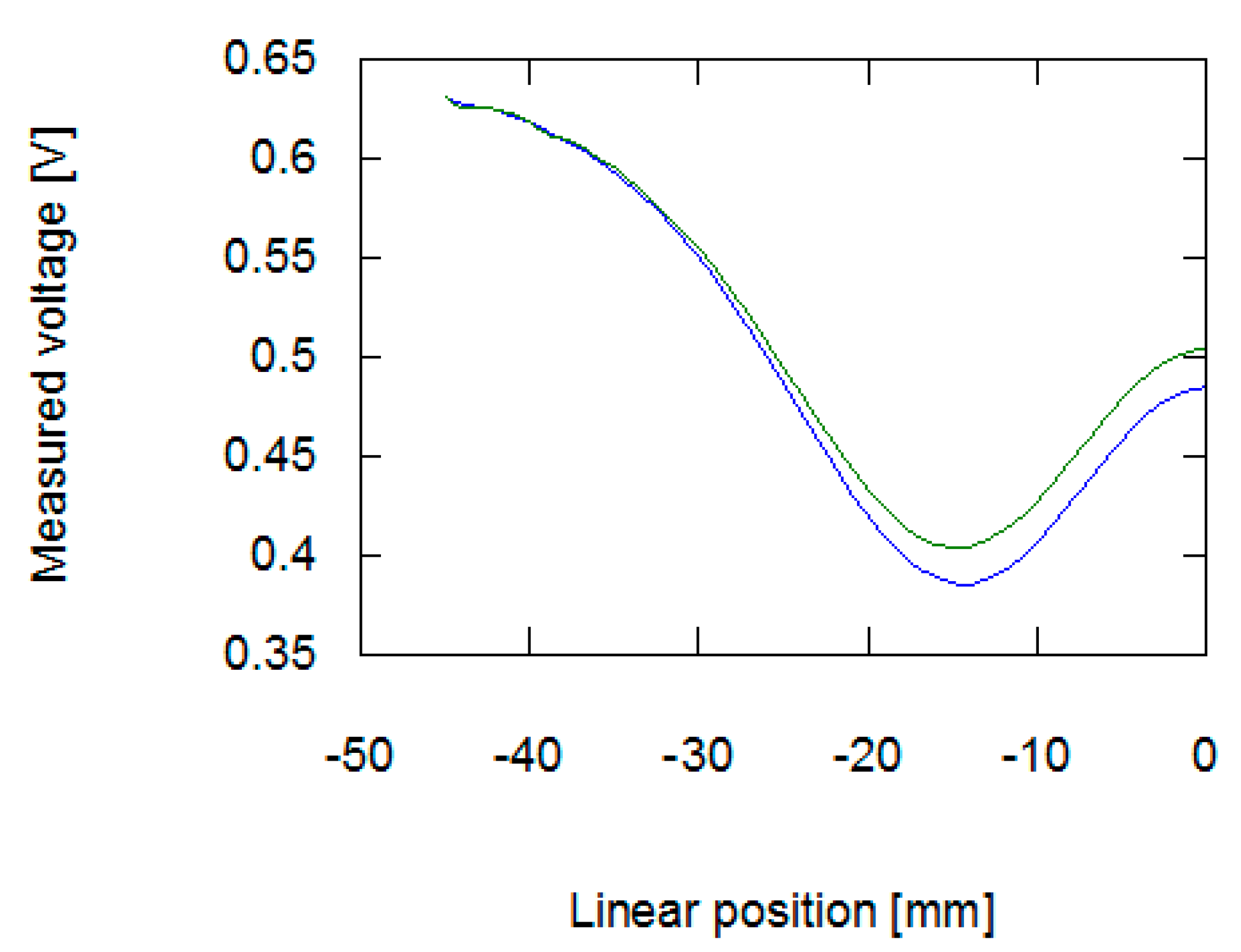
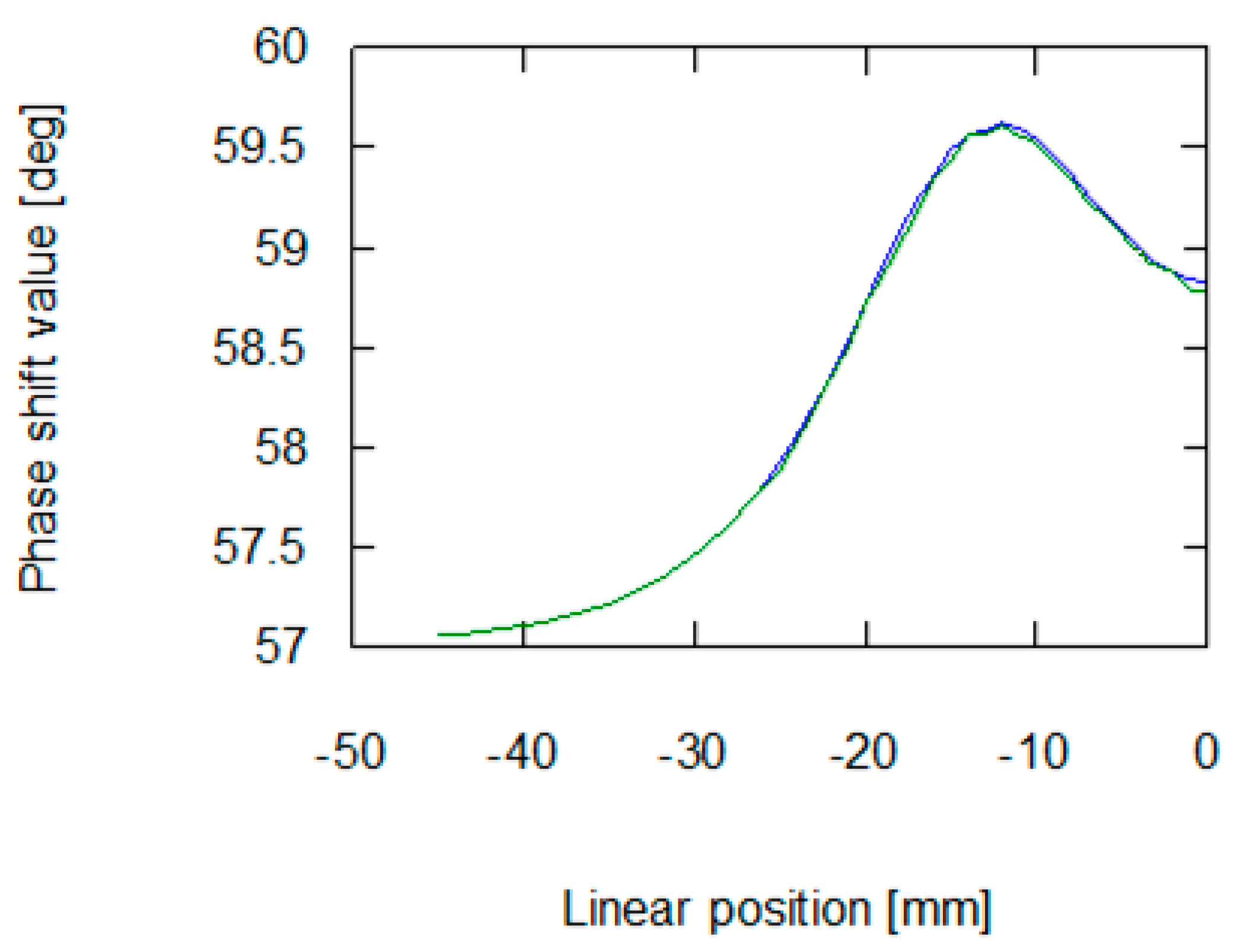
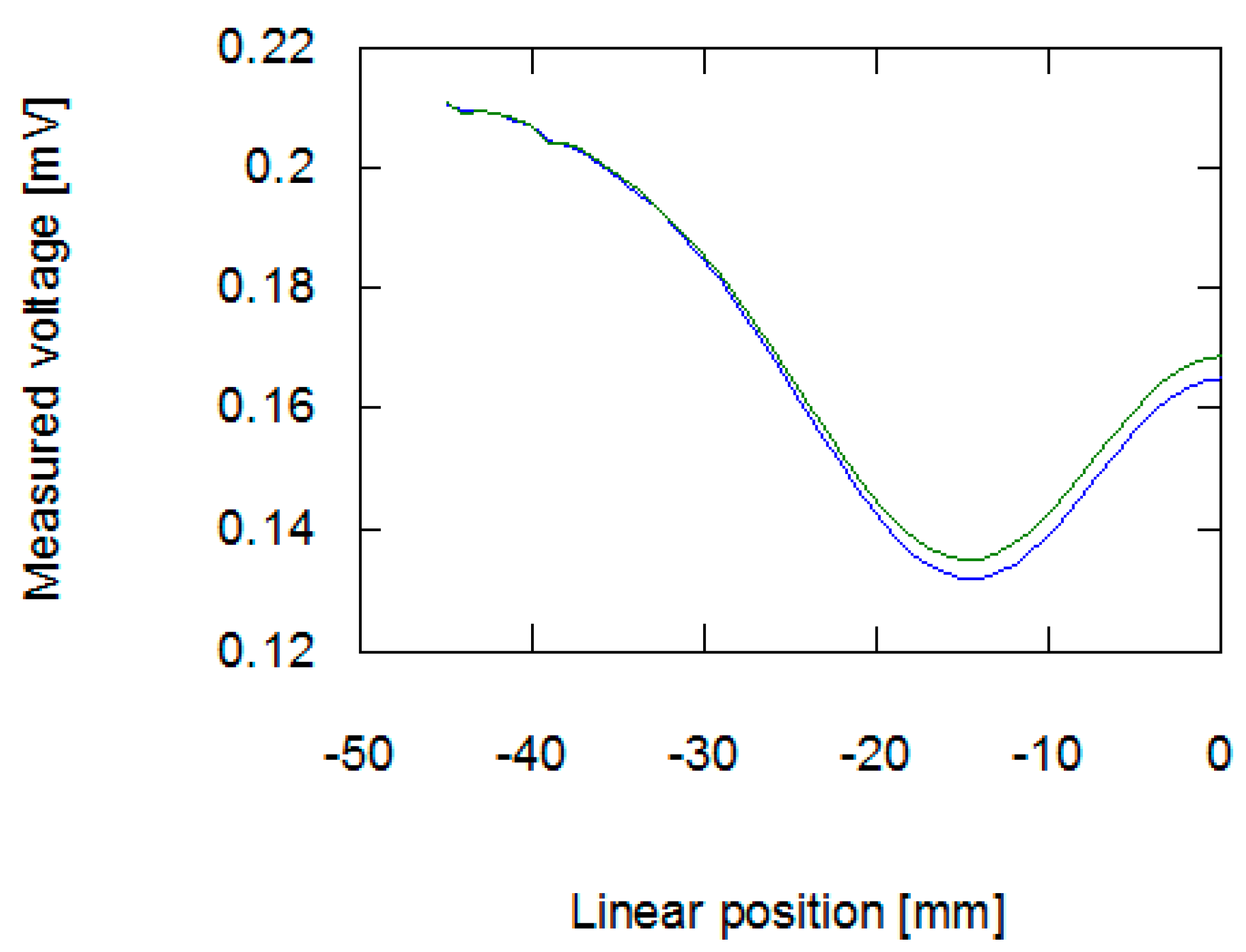
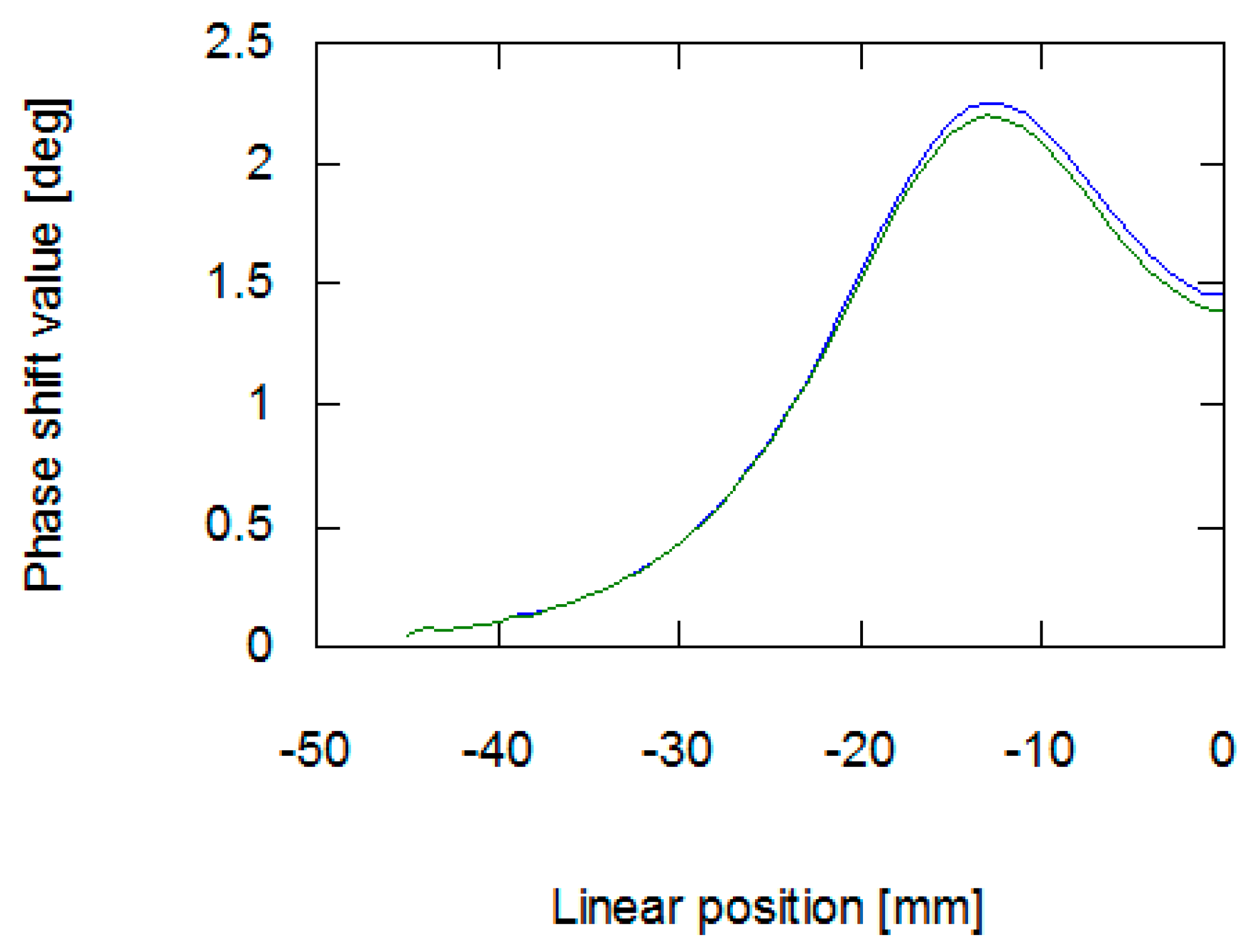
3.1. Measurement Results
3.2. Forward Tomography Transformation Results
3.3. Inverse Tomography Transformation Results
4. Discussion
5. Conclusions
Funding
Conflicts of Interest
References
- Brown, W.F., Jr. Theory of magnetoelastic effects in ferromagnetism. J. Appl. Phys. 1965, 36, 994–1000. [Google Scholar] [CrossRef]
- Du Trémolet de Lacheisserie, E. Magnetostriction: Theory and Applications of Magnetoelasticity, 1st ed.; CRC Press: Boca Raton, FL, USA, 1993; ISBN 9780849369346. [Google Scholar]
- Charubin, T.; Nowicki, M.; Szewczyk, R. Spectral analysis of Matteucci effect based magnetic field sensor. AIP Conf. Proc. 2018, 1996, 020019-1–020019-4. [Google Scholar] [CrossRef]
- Ngaoka, H.; Honda, K. On magnetostriction. Philos. Mag. 1898, 46, 261–290. [Google Scholar] [CrossRef]
- Villari, E. Change of magnetization by tension and by electric current. Annu. Rev. Phys. Chem. 1865, 126, 87–122. [Google Scholar] [CrossRef]
- Xu, J.; Wu, X.; Cheng, C.; Ben, A. A Magnetic Flux Leakage and Magnetostrictive Guided Wave Hybrid Transducer for Detecting Bridge Cables. Sensors 2014, 12, 518–533. [Google Scholar] [CrossRef] [PubMed]
- Jackiewicz, D.; Szewczyk, R.; Bieńkowski, A. Utilizing magnetoelastic effect to monitor the stress in the steel truss structures. JEE 2015, 66, 178–181. [Google Scholar]
- Szewczyk, R. Stress-induced anisotropy and stress dependence of saturation magnetostriction in the Jiles-Atherton-Sablik model of the magnetoelastic Villari effect. Arch. Metall. Mater. 2016, 61, 607–612. [Google Scholar] [CrossRef]
- Salach, J.; Szewczyk, R.; Bienkowski, A.; Kolano-Burian, A.; Falkowski, M. New Method of Measurement of the Magnetoelastic Characteristics for Tensile Stresses. Acta Phys. Pol. A 2010, 118, 775–777. [Google Scholar] [CrossRef]
- Cappello, C.; Zonta, D.; Ait Laasri, H.; Glisic, B.; Wang, M. Calibration of Elasto-Magnetic Sensors on In-Service Cable-Stayed Bridges for Stress Monitoring. Sensors 2018, 18, 466. [Google Scholar] [CrossRef] [PubMed]
- Premel, D.; Mohammad-Djafari, A. Eddy current tomography in cylindrical geometry. IEEE Trans. Magn. 1995, 31, 2000–2003. [Google Scholar] [CrossRef]
- Soleimani, M.; Tamburrino, A. Shape reconstruction in magnetic induction tomography using multifrequency data. Int. J. Inf. Syst. Sci. 2006, 2, 343–353. [Google Scholar]
- Salach, J.; Szewczyk, R.; Nowicki, M. Eddy current tomography for testing of ferromagnetic and non-magnetic materials. Meas. Sci. Technol. 2014, 25, 1–4. [Google Scholar] [CrossRef]
- Ito, K.; Jin, B. Inverse Problems: Tikhonov Theory and Algorithms, 1st ed.; World Scientific: Singapore, 2014; ISBN 978-981-4596-21-3. [Google Scholar]
- Ma, L.; Soleimani, M. Magnetic Induction Spectroscopy for Permeability Imaging. Sci. Rep. 2018, 8, 7025. [Google Scholar] [CrossRef] [PubMed]
- Kachniarz, M.; Kołakowska, K.; Salach, J.; Szewczyk, R.; Nowak, P. Magnetoelastic Villari Effect in Structural Steel Magnetized in the Rayleigh Region. Acta Phys. Pol. A 2018, 133, 660–662. [Google Scholar] [CrossRef]
- Råback, P.; Malinen, M.; Ruokolainen, J.; Pursula, A.; Zwinger, T. Elmer Models Manual; CSC–IT Center for Science: Helsinki, Finland, 2013. [Google Scholar]
- Monk, P. Finite Element Methods for Maxwell’s Equations, 1st ed.; Oxford University Press: Oxford, UK, 2003; ISBN 9780198508885. [Google Scholar]
- Szewczyk, R. Magnetostatic Modelling of Thin Layers Using the Method of Moments and Its Implementation in OCTAVE/MATLAB, 1st ed.; Springer: Berlin, Germany, 2018; ISBN 978-3-319-77985-0. [Google Scholar]
- Nowak, P.; Urbański, M.; Raback, P.; Roukolainen, J.; Kachiarz, M.; Szewczyk, R. Discrete Inverse Transformation for Eddy Current Tomography. Acta Phys. Pol. A 2018, 133, 701–703. [Google Scholar] [CrossRef]
- Nowak, P.; Szewczyk, R. Determination of Initial Parameters for Inverse Tomography Transformation in Eddy Current Tomography. In Automation 2018 Advances in Automation, Robotics and Measurement Techniques, 1st ed.; Szewczyk, R., Zieliński, C., Kaliczyńska, M., Eds.; Springer: Berlin, Germany, 2018; Volume 1, pp. 682–688. ISBN 978-3-319-77179-3. [Google Scholar]
- Nelder, J.; Mead, R. A simplex method for function minimization. Comput. J. 1965, 7, 308–313. [Google Scholar] [CrossRef]


| Sample Stresses (mpa) | M Value Obtained from Inverse Tomography Transformation | M Value Obtained with Standard Method | Relative Error (%) |
|---|---|---|---|
| 0 | 81.2 | 80 | 1.5 |
| 30 | 68.1 | 66.8 | 1.9 |
© 2019 by the author. Licensee MDPI, Basel, Switzerland. This article is an open access article distributed under the terms and conditions of the Creative Commons Attribution (CC BY) license (http://creativecommons.org/licenses/by/4.0/).
Share and Cite
Nowak, P. Magnetoelastic Effect Detection with the Usage of Eddy Current Tomography. Materials 2019, 12, 346. https://doi.org/10.3390/ma12030346
Nowak P. Magnetoelastic Effect Detection with the Usage of Eddy Current Tomography. Materials. 2019; 12(3):346. https://doi.org/10.3390/ma12030346
Chicago/Turabian StyleNowak, Paweł. 2019. "Magnetoelastic Effect Detection with the Usage of Eddy Current Tomography" Materials 12, no. 3: 346. https://doi.org/10.3390/ma12030346
APA StyleNowak, P. (2019). Magnetoelastic Effect Detection with the Usage of Eddy Current Tomography. Materials, 12(3), 346. https://doi.org/10.3390/ma12030346