2D–3D Digital Image Correlation Comparative Analysis for Indentation Process

 , ,
, ,  , and
, and 
Abstract
1. Introduction
- : correlation function.
- : pixel coordinates values in the reference image.
- : displacement in x and y coordinates.
- n/2: should be taken as an integer.
- : value associated to pixel in position (reference image).
- : value associated to pixel in position (deformed image).
- : pixel values of image before deformation.
- : pixel values of image after deformation.
- is the mapped position of Q point.
- is the position of Q point in the reference image.
- are the first-order displacement gradients of the reference subset.
- ∆x is the x distance between Q and P points in the reference subset.
- ∆y is the y distance between Q and P points in the reference subset.
- and are the longitudinal strains in x and y directions, respectively.
- is the angular strain.
2. Materials and Methods
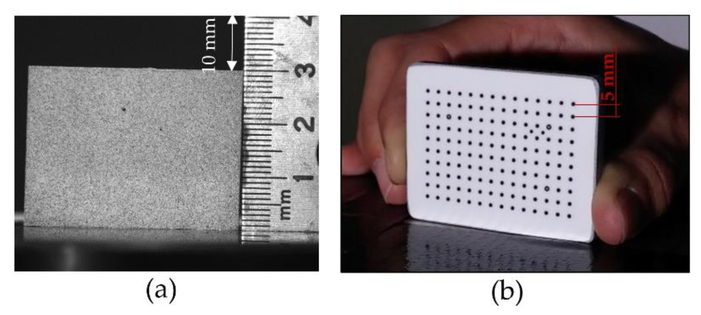
2.1. Materials and Specimens
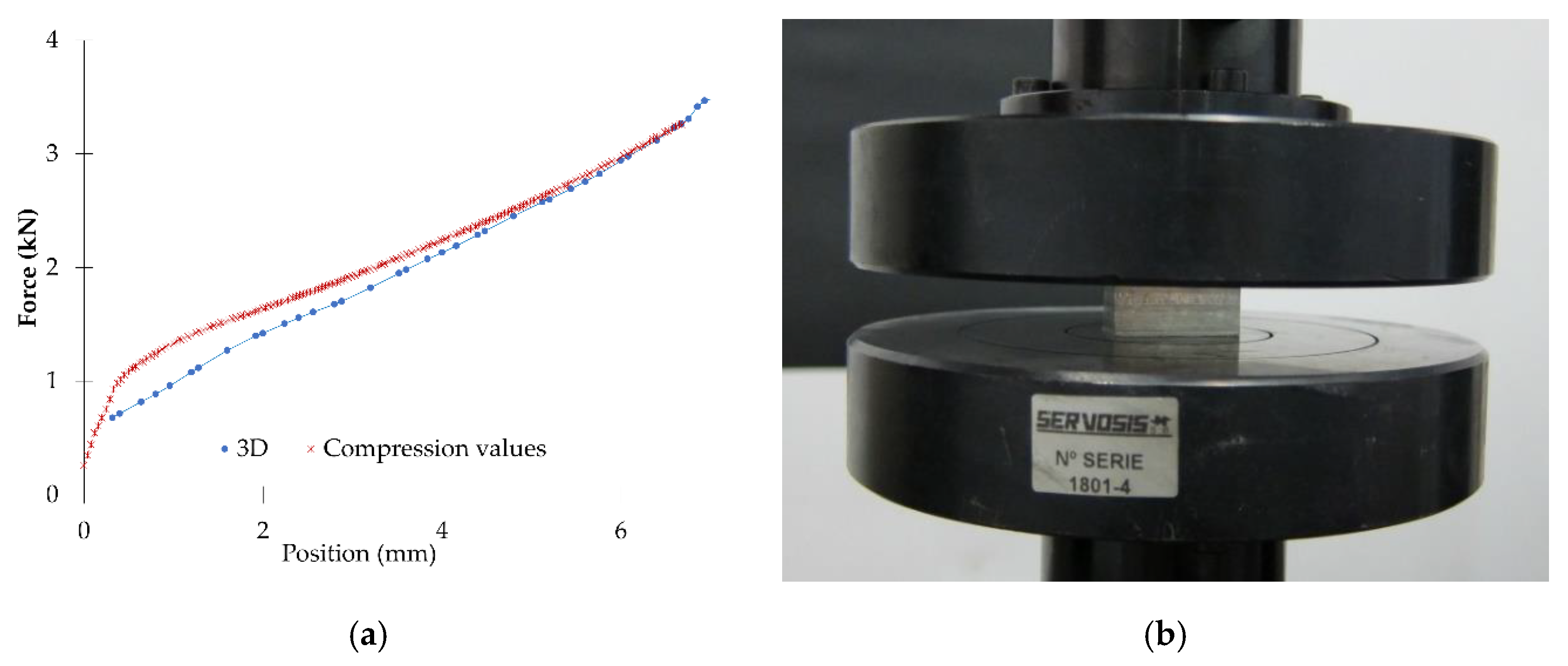
2.2. Equipment
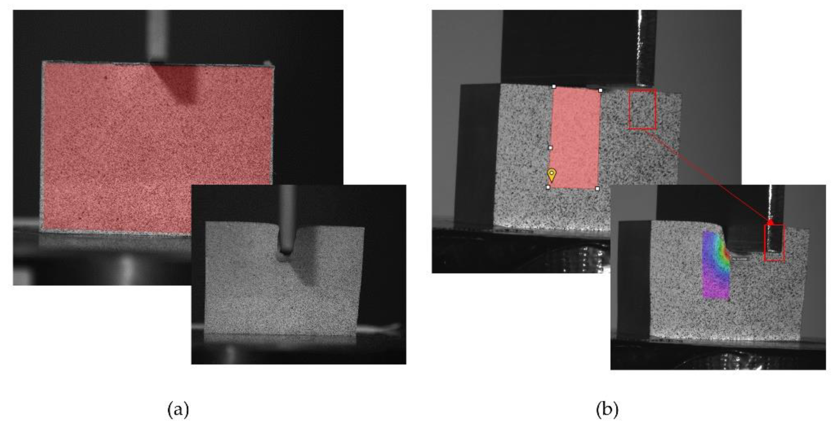
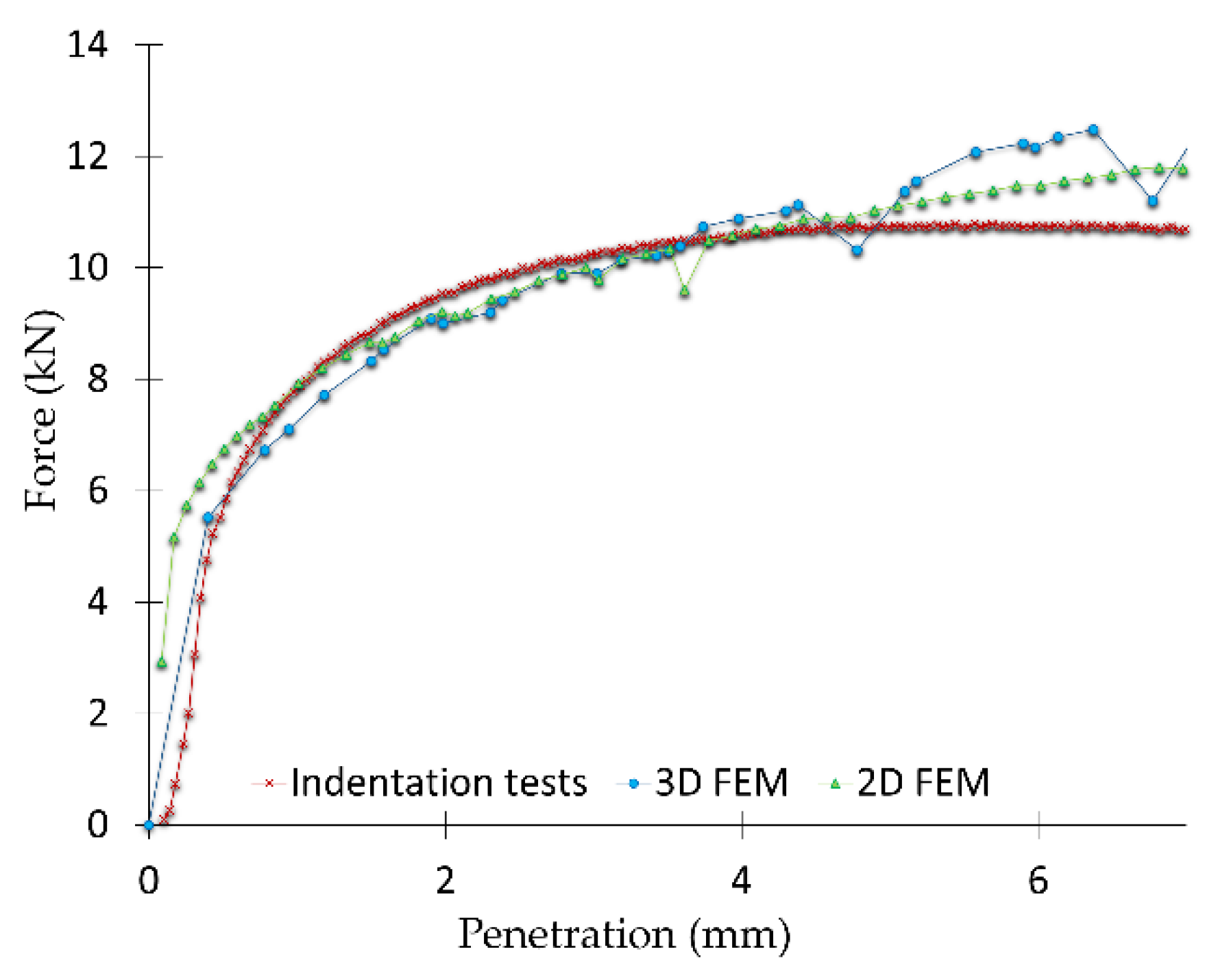
3. Results
4. Conclusions
Author Contributions
Funding
Acknowledgments
Conflicts of Interest
References
- Wagih, A.; Attia, M.A.; AbdelRahman, A.A.; Bendine, K.; Sebaey, T.A. On the indentation of elastoplastic functionally graded materials. Mech. Mater. 2019, 129, 169–188. [Google Scholar] [CrossRef]
- Huang, L.Y.; Guan, K.S.; Xu, T.; Zhang, J.M.; Wang, Q.Q. Investigation of the mechanical properties of steel using instrumented indentation test with simulated annealing particle swarm optimization. Theor. Appl. Fract. Mech. 2019, 102, 116–121. [Google Scholar] [CrossRef]
- Wu, S.B.; Guan, K.S. Evaluation of tensile properties of austenitic stainless steel 316L with linear hardening by modified indentation method. Mater. Sci. Technol. 2014, 30, 1404–1409. [Google Scholar] [CrossRef]
- Udalov, A.; Parshin, S.; Udalov, A. Indentation size effect during measuring the hardness of materials by pyramidal indenter. Mater. Today Proc. 2019. [Google Scholar] [CrossRef]
- Suresh, K.; Kumar, P.G.; Priyadarshini, A.; Kotkunde, N. Analysis of formability in incremental forming processes. Mater. Today Proc. 2018, 5, 18905–18910. [Google Scholar] [CrossRef]
- Bouhamed, A.; Jrad, H.; Mars, J.; Wali, M.; Gamaoun, F.; Dammak, F. Homogenization of elasto-plastic functionally graded material based on representative volume element: Application to incremental forming process. Int. J. Mech. Sci. 2019, 160, 412–420. [Google Scholar] [CrossRef]
- Ambrogio, G.; Palumbo, G.; Sgambitterra, E.; Guglielmi, P.; Piccininni, A.; De Napoli, L.; Villa, T.; Fragomeni, G. Experimental investigation of the mechanical performances of titanium cranial prostheses manufactured by super plastic forming and single-point incremental forming. Int. J. Adv. Manuf. Technol. 2018, 98, 1489–1503. [Google Scholar] [CrossRef]
- Palumbo, G.; Brandizzi, M. Experimental investigations on the single point incremental forming of a titanium alloy component combining static heating with high tool rotation speed. Mater. Des. 2012, 40, 43–51. [Google Scholar] [CrossRef]
- Fragapane, S.; Giallanza, A.; Cannizzaro, L.; Pasta, A.; Marannano, G. Experimental and numerical analysis of aluminum-aluminum bolted joints subject to an indentation process. Int. J. Fatigue. 2015, 80, 332–340. [Google Scholar] [CrossRef]
- Marannano, G.; Virzì Mariotti, G.; D’Acquisto, L.; Restivo, G.; Gianaris, N. Effect of Cold Working and Ring Indentation on Fatigue Life of Aluminum Alloy Specimens. Exp. Tech. 2015, 39, 19–27. [Google Scholar] [CrossRef]
- Groche, P.; Fritsche, D.; Tekkaya, E.A.; Allwood, J.M.; Hirt, G.; Neugebauer, R. Incremental Bulk Metal Forming. CIRP Ann. Manuf. Technol. 2007, 56, 635–656. [Google Scholar] [CrossRef]
- Wernicke, S.; Gies, S.; Tekkaya, A.E. Manufacturing of hybrid gears by incremental sheet-bulk metal forming. Procedia Manuf. 2019, 27, 152–157. [Google Scholar] [CrossRef]
- Sieczkarek, P.; Wernicke, S.; Gies, S.; Tekkaya, A.E.; Krebs, E.; Wiederkehr, P.; Biermann, D.; Tillmann, W.; Stangier, D. Improvement strategies for the formfilling in incremental gear forming processes. Prod. Eng. 2017, 11, 623–631. [Google Scholar] [CrossRef]
- Pilz, F.; Merklein, M. Comparison of extrusion processes in sheet-bulk metal forming for production of filigree functional elements. CIRP J. Manuf. Sci. Technol. 2019. [Google Scholar] [CrossRef]
- Bermudo, C.; Sevilla, L.; Martín, F.; Trujillo, F.J. Hardening effect analysis by modular upper bound and finite element methods in indentation of aluminum, steel, titanium and superalloys. Materials 2017, 10, 556. [Google Scholar] [CrossRef] [PubMed]
- Moncada, A.; Martín, F.; Sevilla, L.; Camacho, A.M.; Sebastián, M.A. Analysis of Ring Compression Test by Upper Bound Theorem as Special Case of Non-symmetric Part. Procedia Eng. 2015, 132, 334–341. [Google Scholar] [CrossRef]
- Wu, Y.; Dong, X.; Yu, Q. An upper bound solution of axial metal flow in cold radial forging process of rods. Int. J. Mech. Sci. 2014, 85, 120–129. [Google Scholar] [CrossRef]
- Wu, Y.; Dong, X. An upper bound model with continuous velocity field for strain inhomogeneity analysis in radial forging process. Int. J. Mech. Sci. 2016, 115, 385–391. [Google Scholar] [CrossRef]
- López-Chipres, E.; García-Sanchez, E.; Ortiz-Cuellar, E.; Hernandez-Rodriguez, M.A.L.; Colás, R. Optimization of the Severe Plastic Deformation Processes for the Grain Refinement of Al6060 Alloy Using 3D FEM Analysis. J. Mater. Eng. Perform. 2010. [Google Scholar] [CrossRef]
- Hofmeister, B.; Bruns, M.; Rolfes, R. Finite element model updating using deterministic optimisation: A global pattern search approach. Eng. Struct. 2019, 195, 373–381. [Google Scholar] [CrossRef]
- Skozrit, I.; Frančeski, J.; Tonković, Z.; Surjak, M.; Krstulović-Opara, L.; Vesenjak, M.; Kodvanj, J.; Gunjević, B.; Lončarić, D. Validation of Numerical Model by Means of Digital Image Correlation and Thermography. Procedia Eng. 2015, 101, 450–458. [Google Scholar] [CrossRef]
- Pan, B.; Qian, K.; Xie, H.; Asundi, A. Two-dimensional digital image correlation for in-plane displacement and strain measurement: A review. Meas. Sci. Technol. 2009, 20, 062001. [Google Scholar] [CrossRef]
- Bermudo, C.; Sevilla, L.; Castillo, G. Material flow analysis in indentation by two-dimensional digital image correlation and finite elements method. Materials 2017, 10, 674. [Google Scholar] [CrossRef] [PubMed]
- Sousa, P.J.; Barros, F.; Tavares, P.J. Displacement measurement and shape acquisition of an RC helicopter blade using Digital Image Correlation. Procedia Struct. Integr. 2017, 5, 1253–1259. [Google Scholar] [CrossRef]
- Ho, C.-C.; Chang, Y.-J.; Hsu, J.-C.; Kuo, C.-L.; Kuo, S.-K.; Lee, G.-H. Residual Strain Measurement Using Wire EDM and DIC in Aluminum. Inventions 2016, 1, 4. [Google Scholar] [CrossRef]
- Bruck, H.A.; McNeill, S.R.; Sutton, M.A.; Peters, W.H. Digital image correlation using Newton-Raphson method of partial differential correction. Exp. Mech. 1989, 29, 261–267. [Google Scholar] [CrossRef]
- Park, J.; Yoon, S.; Kwon, T.-H.; Park, K. Assessment of speckle-pattern quality in digital image correlation based on gray intensity and speckle morphology. Opt. Lasers Eng. 2017, 91, 62–72. [Google Scholar] [CrossRef]
- Roux, S.; Réthoré, J.; Hild, F. Digital image correlation and fracture: An advanced technique for estimating stress intensity factors of 2D and 3D cracks. J. Phys. D. Appl. Phys. 2009, 42, 214004. [Google Scholar] [CrossRef]
- Lin, Q.; Wan, B.; Wang, Y.; Lu, Y.; Labuz, J.F. Unifying acoustic emission and digital imaging observations of quasi-brittle fracture. Theor. Appl. Fract. Mech. 2019, 103, 102301. [Google Scholar] [CrossRef]
- Hao Kan, W.; Albino, C.; Dias-da-Costa, D.; Dolman, K.; Lucey, T.; Tang, X.; Cairney, J.; Proust, G. Fracture toughness testing using photogrammetry and digital image correlation. MethodsX 2018, 5, 1166–1177. [Google Scholar] [CrossRef]
- Bertelsen, I.M.G.; Kragh, C.; Cardinaud, G.; Ottosen, L.M.; Fischer, G. Quantification of plastic shrinkage cracking in mortars using digital image correlation. Cem. Concr. Res. 2019, 123. [Google Scholar] [CrossRef]
- Fayyad, T.M.; Lees, J.M. Application of Digital Image Correlation to reinforced concrete fracture. Procedia Mater. Sci. 2014, 3, 1585–1590. [Google Scholar] [CrossRef]
- Nguyen, V.-T.; Kwon, S.-J.; Kwon, O.-H.; Kim, Y.-S. Mechanical Properties Identification of Sheet Metals by 2D-Digital Image Correlation Method. Procedia Eng. 2017, 184, 381–389. [Google Scholar] [CrossRef]
- del Rey Castillo, E.; Allen, T.; Henry, R.; Griffith, M.; Ingham, J. Digital image correlation (DIC) for measurement of strains and displacements in coarse, low volume-fraction FRP composites used in civil infrastructure. Compos. Struct. 2019, 212, 43–57. [Google Scholar] [CrossRef]
- Kumar, S.L.; Aravind, H.B.; Hossiney, N. Digital Image Correlation (DIC) for measuring strain in brick masonry specimen using Ncorr open source 2D MATLAB program. Results Eng. 2019, 100061. [Google Scholar] [CrossRef]
- Hensley, S.; Christensen, M.; Small, S.; Archer, D.; Lakes, E.; Rogge, R. Digital image correlation techniques for strain measurement in a variety of biomechanical test models. Acta Bioeng. Biomech. 2017, 19, 187–195. [Google Scholar]
- Yang, L.; Smith, L.; Gotherkar, A.; Chen, X. Measure Strain Distribution Using Digital Image Correlation (DIC) for Tensile Tests; Oakland University: Oakland, Rochester, ML, USA, 2010. [Google Scholar]
- Chen, Y.; Wei, J.; Huang, H.; Jin, W.; Yu, Q. Application of 3D-DIC to characterize the effect of aggregate size and volume on non-uniform shrinkage strain distribution in concrete. Cem. Concr. Compos. 2018, 86, 178–189. [Google Scholar] [CrossRef]
- Aydin, M.; Wu, X.; Cetinkaya, K.; Yasar, M.; Kadi, I. Application of Digital Image Correlation technique to Erichsen Cupping Test. Eng. Sci. Technol. Int. J. 2018, 21, 760–768. [Google Scholar] [CrossRef]
- Helfrick, M.N.; Niezrecki, C.; Avitabile, P.; Schmidt, T. 3D digital image correlation methods for full-field vibration measurement. Mech. Syst. Signal Process. 2011, 25, 917–927. [Google Scholar] [CrossRef]
- Molina-Viedma, A.J.; Felipe-Sesé, L.; López-Alba, E.; Díaz, F. High frequency mode shapes characterisation using Digital Image Correlation and phase-based motion magnification. Mech. Syst. Signal Process. 2018, 102, 245–261. [Google Scholar] [CrossRef]
- Guo, X.; Liang, J.; Xiao, Z.; Cao, B. Digital image correlation for large deformation applied in Ti alloy compression and tension test. Opt. Int. J. Light Electron Opt. 2014, 125, 5316–5322. [Google Scholar] [CrossRef]
- Castillo López, G.; Carrasco Vela, G. Correlación numérico-experimental del ensayo de tracción. In XX Congreso Nacional de Ingeniería Mecánica; Universidad de Málaga: Málaga, Spain, 2014. [Google Scholar]
- Correlated Solutions Inc. Digital Image Correlation: Principles and Software; University of South Carolina: Columbia, SC, USA, 2009. [Google Scholar]
- Lakshmi Aparna, M.; Chaitanya, G.; Srinivas, K.; Rao, J.A. Fatigue Testing of Continuous GFRP Composites Using Digital Image Correlation (DIC) Technique a Review. Mater. Today Proc. 2015, 2, 3125–3131. [Google Scholar] [CrossRef]
- Schreier, H.; Orteu, J.-J.; Sutton, M.A. Image Correlation for Shape, Motion and Deformation Measurements; Springer US: Boston, MA, USA, 2009; ISBN 978-0-387-78746-6. [Google Scholar]
- Schreier, H.W.; Sutton, M.A. Systematic errors in digital image correlation due to undermatched subset shape functions. Exp. Mech. 2002, 42, 303–310. [Google Scholar] [CrossRef]
- Correlated Solutions Inc. CSI Application Note AN-525. Speckle Pattern Fundamentals; Correlated Solutions: Irmo, SC, USA, 2009. [Google Scholar]
- Correlated Solutions VIC SNAP. Available online: https://www.correlatedsolutions.com/vic-snap-remote/ (accessed on 10 December 2009).
- Correlated Solutions. VIC-2D Reference Manual; Correlated Solutions: Irmo, SC, USA, 2009; p. 59. [Google Scholar]
- Correlated Solutions. VIC-3D Reference Manual; Correlated Solutions: Irmo, SC, USA, 2018. [Google Scholar]
- Fluhrer, J. Deform. Design Environment for Forging. User’s Manual; Scientific Forming Technologies Corporation: Columbus, OH, USA, 2010. [Google Scholar]
- Bermudo, C.; Sevilla, L.; Martín, F.; Trujillo, F.J. Study of the Tool Geometry Influence in Indentation for the Analysis and Validation of the New Modular Upper Bound Technique. Appl. Sci. 2016, 6, 203. [Google Scholar] [CrossRef]
- Bermudo Gamboa, C. Análisis, Desarrollo y Validación del Método del Límite Superior en Procesos de Conformado por Indentación; Servicio de Publicaciones y Divulgación Científica: Málaga, Spain, 2015. [Google Scholar]


© 2019 by the authors. Licensee MDPI, Basel, Switzerland. This article is an open access article distributed under the terms and conditions of the Creative Commons Attribution (CC BY) license (http://creativecommons.org/licenses/by/4.0/).
Share and Cite
Bermudo Gamboa, C.; Martín-Béjar, S.; Trujillo Vilches, F.J.; Castillo López, G.; Sevilla Hurtado, L. 2D–3D Digital Image Correlation Comparative Analysis for Indentation Process. Materials 2019, 12, 4156. https://doi.org/10.3390/ma12244156
Bermudo Gamboa C, Martín-Béjar S, Trujillo Vilches FJ, Castillo López G, Sevilla Hurtado L. 2D–3D Digital Image Correlation Comparative Analysis for Indentation Process. Materials. 2019; 12(24):4156. https://doi.org/10.3390/ma12244156
Chicago/Turabian StyleBermudo Gamboa, Carolina, Sergio Martín-Béjar, F. Javier Trujillo Vilches, G. Castillo López, and Lorenzo Sevilla Hurtado. 2019. "2D–3D Digital Image Correlation Comparative Analysis for Indentation Process" Materials 12, no. 24: 4156. https://doi.org/10.3390/ma12244156
APA StyleBermudo Gamboa, C., Martín-Béjar, S., Trujillo Vilches, F. J., Castillo López, G., & Sevilla Hurtado, L. (2019). 2D–3D Digital Image Correlation Comparative Analysis for Indentation Process. Materials, 12(24), 4156. https://doi.org/10.3390/ma12244156