Modified Fourier–Galerkin Solution for Aerospace Skin-Stiffener Panels Subjected to Interface Force and Mixed Boundary Conditions

Abstract
1. Introduction
2. Governing Equations of Stiffened Panel and Its Solution Procedure
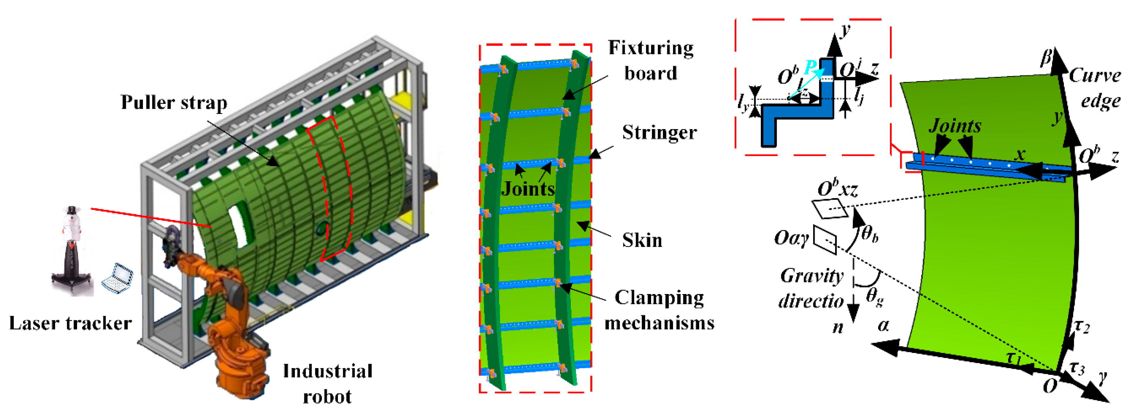
2.1. Shell Subjected to Concentrated Force at Joining Interface and Functional Boundary Conditions
2.2. Fundamental Equation of Spatial Stiffener with Arbitrary Boundaries
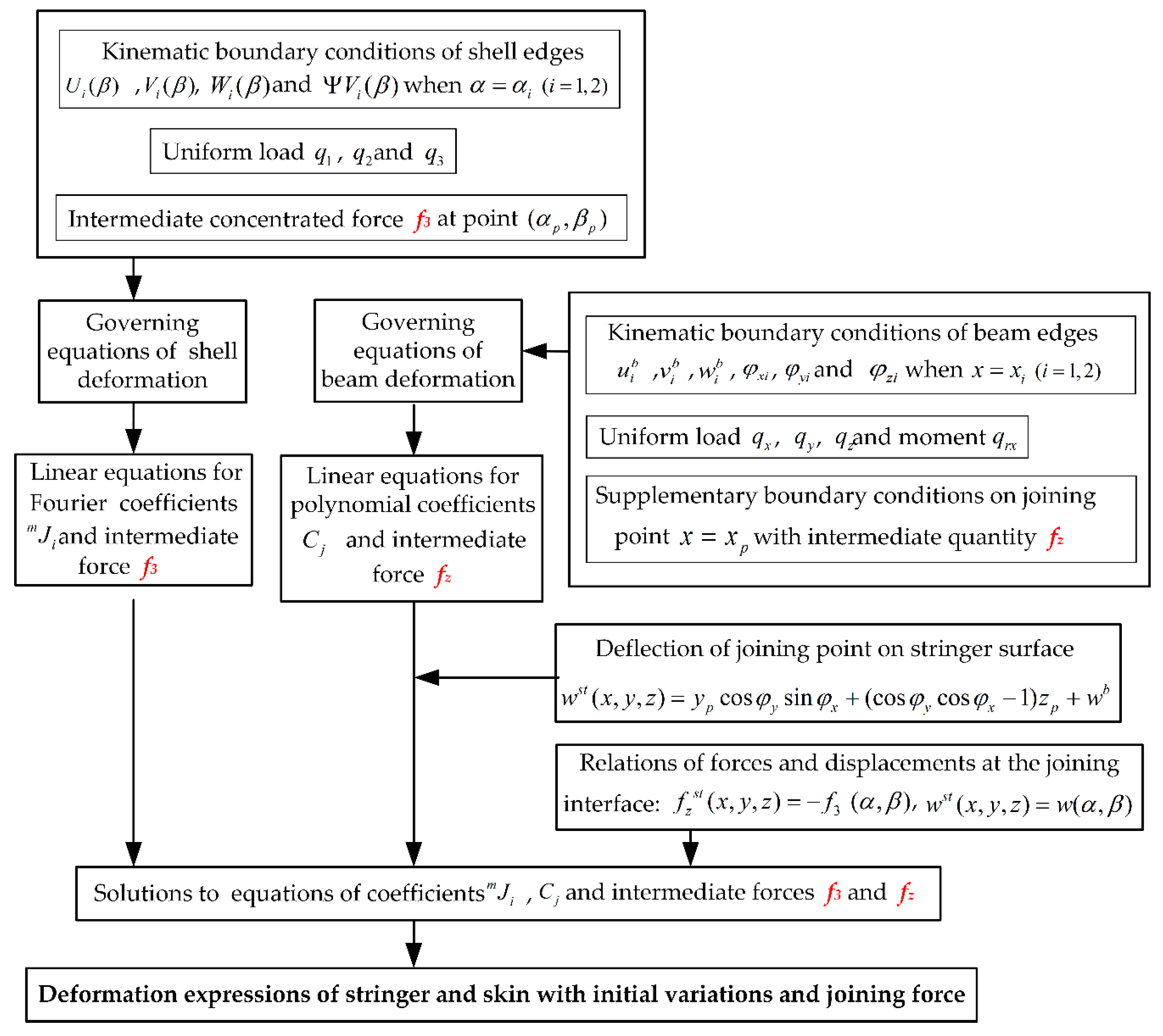
2.3. Calculation Procedure for Stiffened Panel deformation
3. Numerical Validation and Experiments
3.1. Initial Kinematic Boundary Conditions of Panel Components
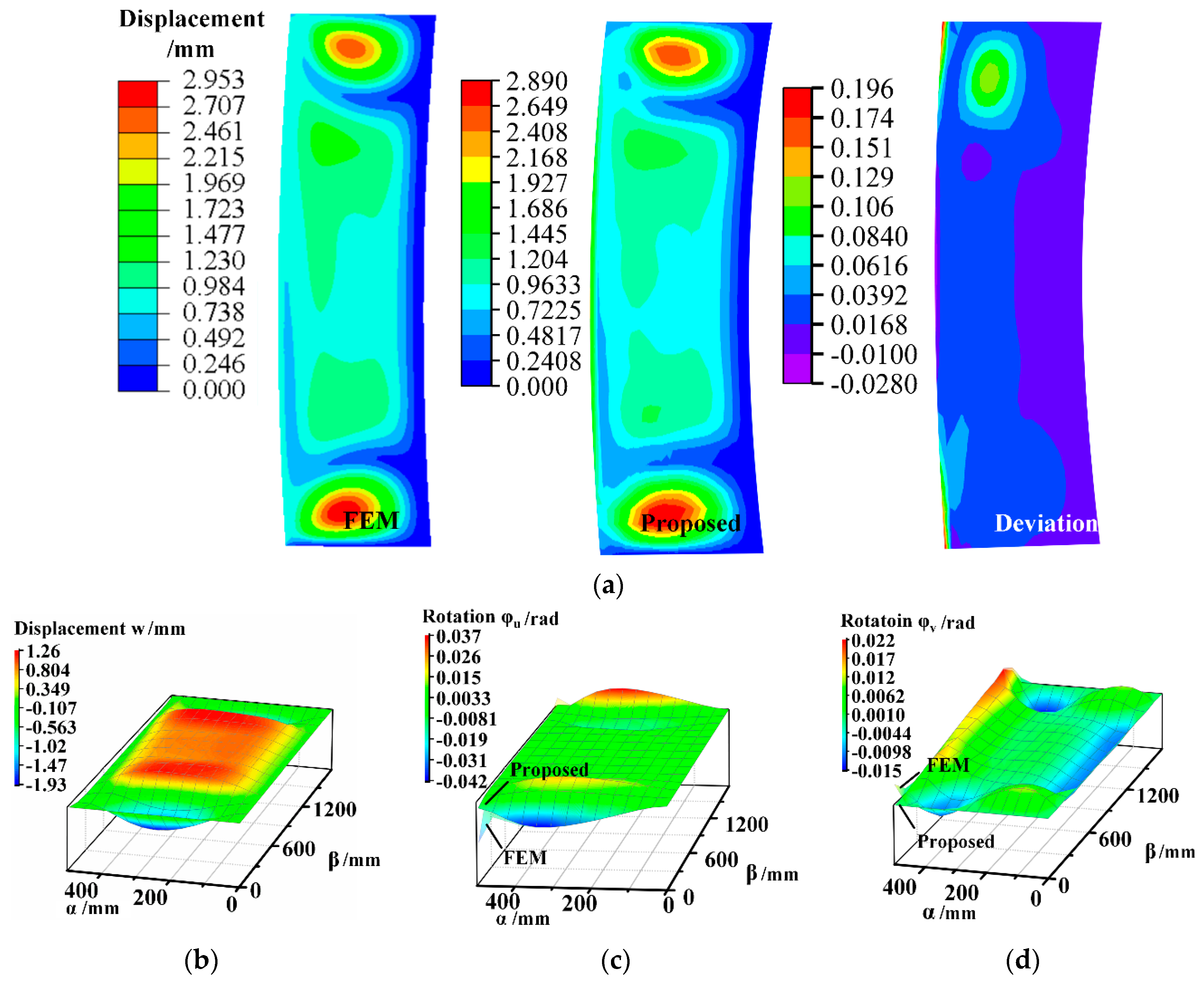
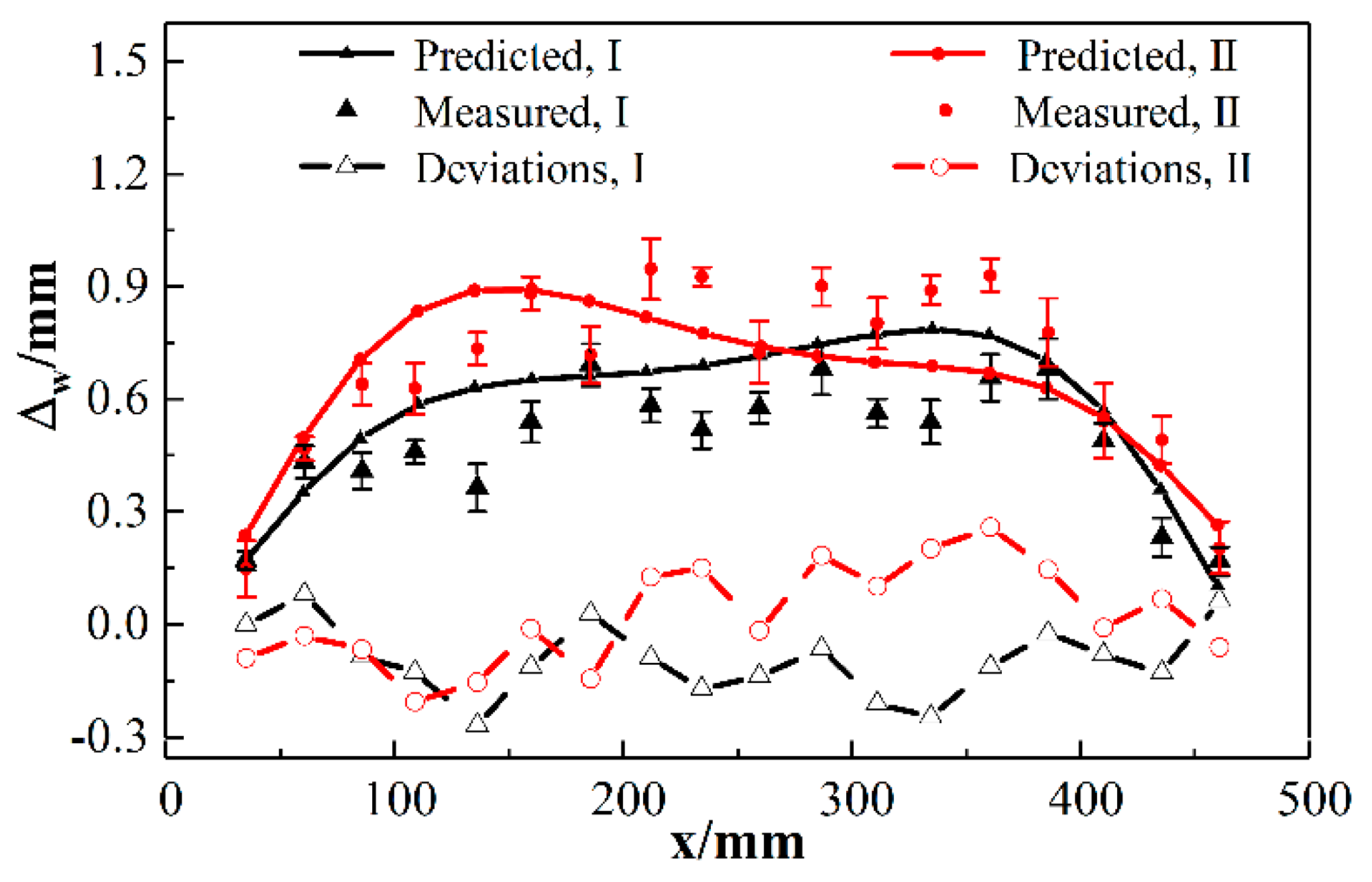
3.2. Initial Deformation of Panel Components
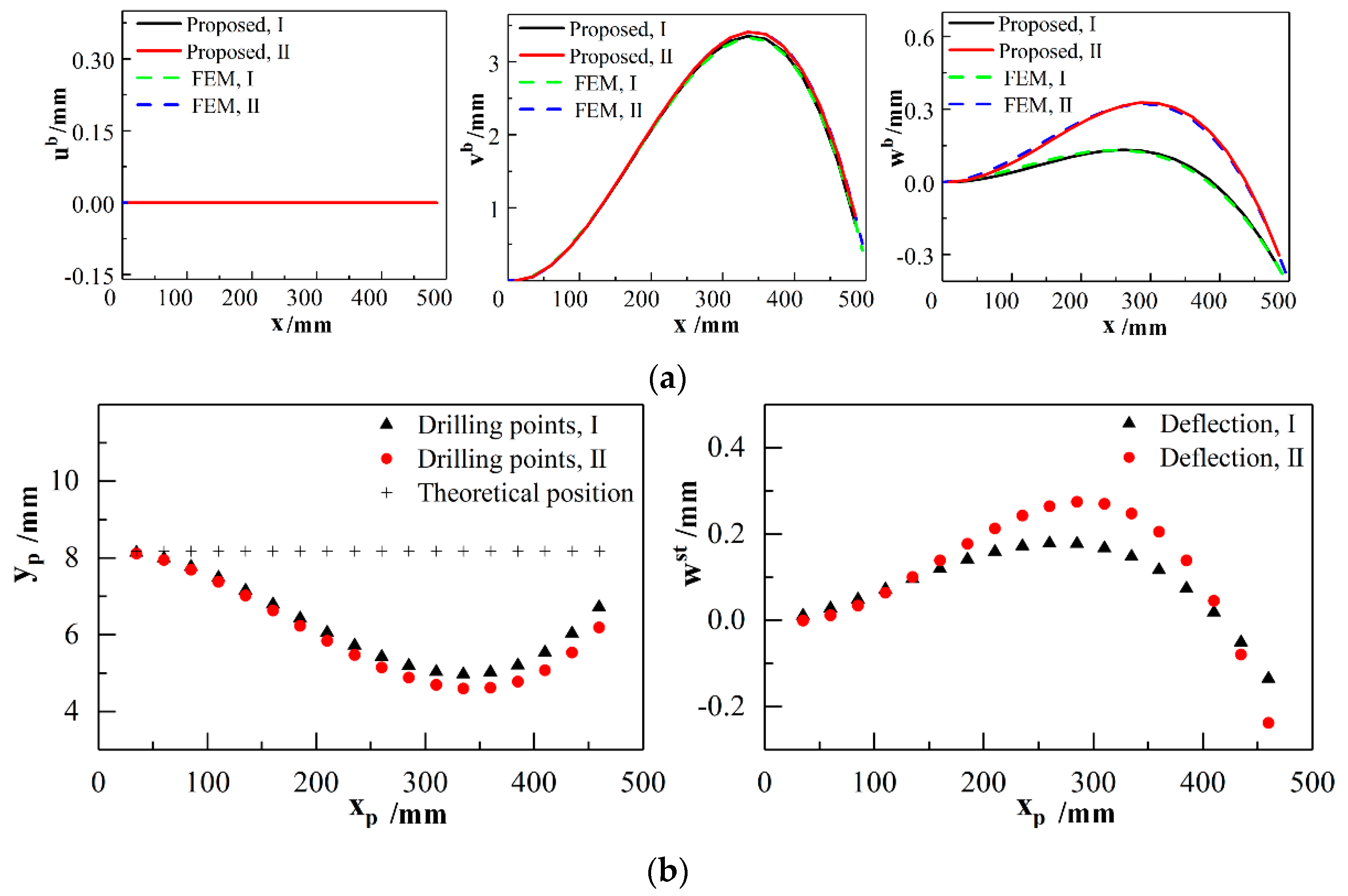
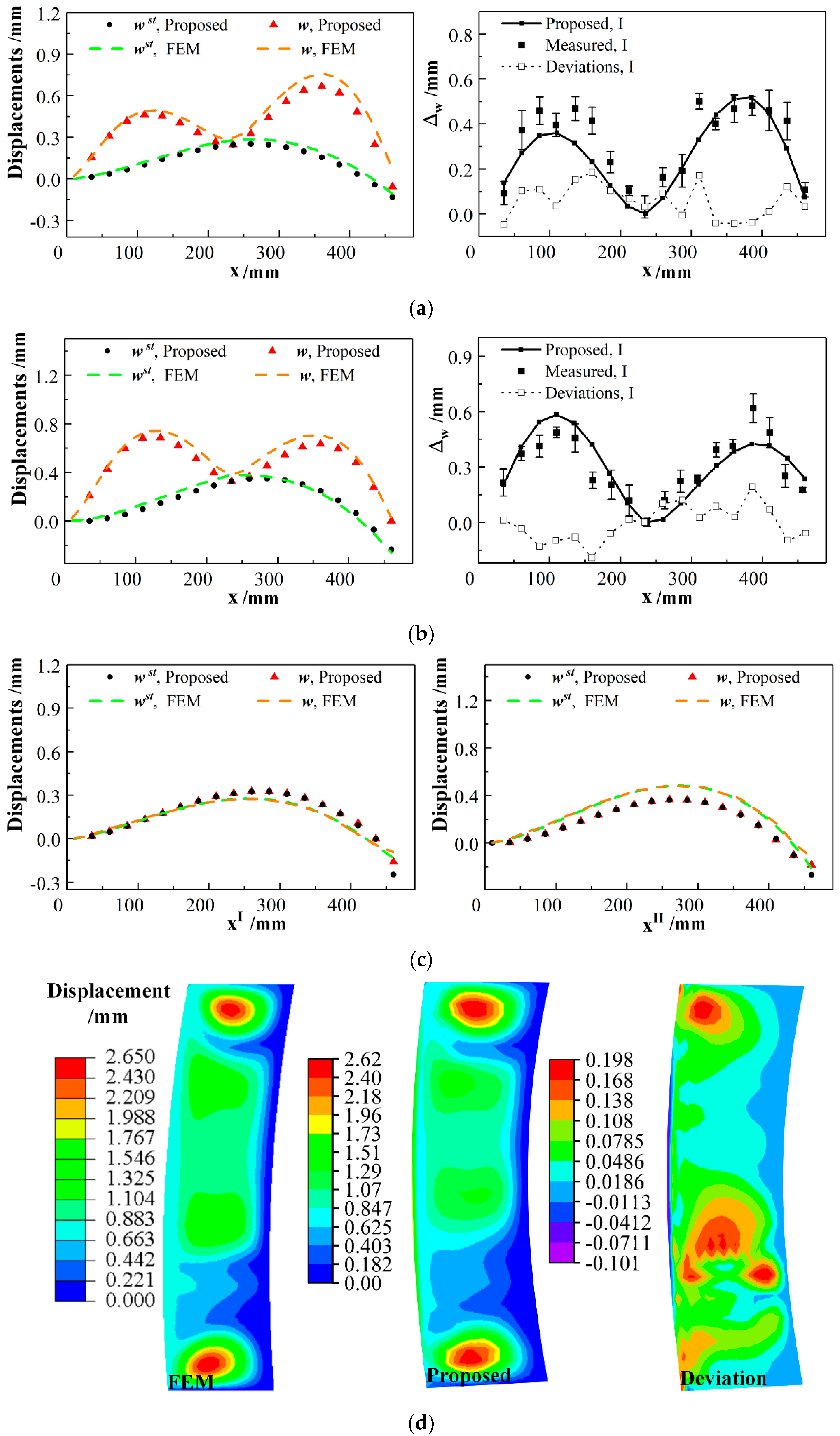
3.3. Deformation of Stiffened Panel with Joints and Mixed Boundary Conditions
4. Conclusions
Author Contributions
Funding
Conflicts of Interest
Nomenclature
| a, b, R, h | length of straight edge and arc edge, curvature radius, shell thickness, mm |
| q1, q2, q3 | external load components in the directions of axes τ1, τ2 and τ3, N·mm−2 |
| qx, qy, qz | external load components along the axes x, y and z, N·mm−1 |
| qrx, qry, qrz | moment components about the axes x, y and z, N·mm |
| f1, f2, f3 | concentrated force components caused by the joining interaction, N |
| N1, N2, N12, N21, Nx | normal internal forces of shell and beam, N·mm−2 |
| M1, M2, M12, M21, My, Mz, Myz | bending and twisting moments, N·mm |
| u, v, w | displacement components of local coordinate system Oτ1τ2τ3, mm |
| φu, φv | rotations around curvilinear coordinates, rad |
| ub, vb, wb | displacements along the centroid locus of the cross-section of beam, mm |
| ust, vst, wst | displacements of point P on the cross-section of the stringer, mm |
| xp, yp, zp | Coordinates of P with respect to Cartesian coordinate system Obxyz, mm |
| σ1, σ2, σ12 | normal stresses and shear stress components, N·mm−2 |
| E, Eb | modulus of elasticity of shell and beam, GPa |
| μ, μb | Poisson’s ratio |
| ρ, ρb | density, kg·m−3 |
| A, as | cross-sectional area, mm2, length of the stiffener, mm |
| Ixx, Iyy, Izz, Iyz, Izy | geometric torsional stiffness and moments of inertia for cross-section area, mm4 |
Appendix A
References
- Tamijani, A.Y.; Kapania, R.K. Buckling and Static Analysis of Curvilinearly Stiffened Plates Using Mesh-Free Method. AIAA J. 2010, 48, 2739–2751. [Google Scholar] [CrossRef]
- Rodcheuy, N.; Frostig, Y.; Kardomateas, G.A. Extended High-Order Theory for Curved Sandwich Panels and Comparison with Elasticity. J. Appl. Mech. 2017, 84, 081002. [Google Scholar] [CrossRef]
- Reddy, J.N. Nonlocal Nonlinear Formulations for Bending of Classical and Shear Deformation Theories of Beams and Plates. Int. J. Eng. Sci. 2010, 48, 1507–1518. [Google Scholar] [CrossRef]
- Fernandes, R.R.; Tamijani, A.Y. Flutter Analysis of Laminated Curvilinear-Stiffened Plates. AIAA J. 2017, 55, 998–1011. [Google Scholar] [CrossRef]
- Su, W.; Cesnik, C.E.S. Strain-Based Geometrically Nonlinear Beam Formulation for Modeling Very Flexible Aircraft. Int. J. Solids Struct. 2011, 48, 2349–2360. [Google Scholar] [CrossRef]
- Carrera, E.; Pagani, A.; Petrolo, M. Component-Wise Method Applied to Vibration of Wing Structures. J. Appl. Mech. 2013, 80, 041012. [Google Scholar] [CrossRef]
- Salehi, M.; Sideris, P. A Finite-Strain Gradient-Inelastic Beam Theory and a Corresponding Force-Based Frame Element Formulation. Int. J. Numer. Methods Eng. 2018, 116, 380–411. [Google Scholar] [CrossRef]
- Tamijani, A.Y.; Kapania, R.K. Chebyshev-Ritz Approach to Buckling and Vibration of Curvilinearly Stiffened Plate. AIAA J. 2012, 50, 1007–1018. [Google Scholar] [CrossRef]
- Carrera, E.; Zappino, E. Carrera Unified Formulation for Free-Vibration Analysis of Aircraft Structures. AIAA J. 2016, 54, 280–292. [Google Scholar] [CrossRef]
- Sobota, P.M.; Dornisch, W.; Muller, R.; Klinkel, S. Implicit Dynamic Analysis Using an Isogeometric Reissner-Mindlin Shell Formulation. Int. J. Numer. Methods Eng. 2017, 110, 803–825. [Google Scholar] [CrossRef]
- Ventsel, E.; Krauthammer, T. Thin Plates and Shells: Theory, Analysis, and Applications; CRC Press: New York, NY, USA, 2001; pp. 319–332. [Google Scholar]
- Zappino, E.; Carrera, E. Multidimensional Model for the Stress Analysis of Reinforced Shell Structures. AIAA J. 2018, 56, 1647–1661. [Google Scholar] [CrossRef]
- Guida, M.; Marulo, F.; Abrate, S. Advances in Crash Dynamics for Aircraft Safety. Prog. Aerosp. Sci. 2018, 98, 106–123. [Google Scholar] [CrossRef]
- Silva, P.B.; Mencik, J.M.; Arruda, J.R.D. Wave Finite Element-Based Superelements for Forced Response Analysis of Coupled Systems via Dynamic Substructuring. Int. J. Numer. Methods Eng. 2016, 107, 453–476. [Google Scholar] [CrossRef]
- Pacheco, D.R.Q.; Marques, F.D.; Ferreira, A.J.M. Finite Element Analysis of Fluttering Plates Reinforced by Flexible Beams: An Energy-Based Approach. J. Sound Vib. 2018, 435, 135–148. [Google Scholar] [CrossRef]
- Slemp, W.C.H.; Kapania, R.K.; Mulani, S.B. Integrated Local Petrov-Galerkin Sinc Method for Structural Mechanics Problems. AIAA J. 2010, 48, 1141–1155. [Google Scholar] [CrossRef]
- Sapountzakis, E.J.; Mokos, V.G. An Improved Model for the Analysis of Plates Stiffened by Parallel Beams with Deformable Connection. Comput. Struct. 2008, 86, 2166–2181. [Google Scholar] [CrossRef]
- Ahmad, N.; Kapania, R.K. Free Vibration Analysis of Integrally Stiffened Plates with Plate-Strip Stiffeners. AIAA J. 2016, 54, 1103–1115. [Google Scholar] [CrossRef]
- Timoshenko, S.; Woinowsky-Krieger, S. Theory of Plates and Shells, 2nd ed.; McGraw-Hill: Singapore, 1959; p. 513. [Google Scholar]
- Wang, Q.; Hou, R.; Li, J.; Ke, Y. Analytical and Experimental Study on Deformation of Thin-Walled Panel with Non-ideal Boundary Conditions. Int. J. Mech. Sci. 2018, 149, 298–310. [Google Scholar] [CrossRef]
- Carrera, E.; Giunta, G.; Petrolo, M. Beam Structures: Classical and Advanced Theories; John Wiley & Sons: Chichester, UK, 2011; pp. 12–15. [Google Scholar]
- Przemieniecki, J.S. Theory of Matrix Structural Analysis; Dover Publications: New York, NY, USA, 1968; pp. 70–76. [Google Scholar]
- Shabana, A.A.; Yakoub, R.Y. Three Dimensional Absolute Nodal Coordinate Formulation for Beam Elements: Theory. J. Mech. Des. 2001, 123, 606–613. [Google Scholar] [CrossRef]
- Wang, Q.; Hou, R.; Li, J.; Ke, Y.; Maropoulos, P.G.; Zhang, X. Positioning Variation Modeling for Aircraft Panels Assembly Based on Elastic Deformation Theory. Proc. Inst. Mech. Eng. Part B J. Eng. Manuf. 2018, 232, 2592–2604. [Google Scholar] [CrossRef]


| Stringer | as/mm | lj/mm | A/mm2 | Iyy/mm4 | Izz/mm4 | Iyz/mm4 | Eb/GPa | ρb/kg·m−3 | θb/rad |
|---|---|---|---|---|---|---|---|---|---|
| I | 495 | 10 | 166.5 | 23420 | 14270 | −14030 | 72 | 2830 | 0.13614 |
| II | 0.19897 |
| R/mm | a/mm | b/mm | h/mm | μ | E/GPa | ρ/kg·m−3 | θg/rad |
|---|---|---|---|---|---|---|---|
| 2724 | 495.5 | 1794.26 | 2 | 0.33 | 73 | 2780 | 1.2415 |
| α/mm | Δτ1/mm | Δτ2/mm | Δτ3/mm | φ1/rad | φ2/rad | φ3/rad |
|---|---|---|---|---|---|---|
| 495.5 | 494.954 | 0.392835 | −0.457491 | −0.004490 | −0.000188 | −0.039646 |
| Stringer | x/mm | Δx/mm | Δy/mm | Δz/mm | φx/rad | φy/rad | φz/rad |
|---|---|---|---|---|---|---|---|
| I | 10 | 0 | 0 | 0 | 0 | 0 | 0 |
| 484.976 | −3.8 × 10⁻⁶ | 0.781103 | −0.356041 | 0.01601 | 0.005193 | −0.039305 | |
| II | 10 | 0 | 0 | 0 | 0 | 0 | 0 |
| 485.013 | 3.1 × 10⁻⁵ | 0.891975 | −0.302205 | −0.01852 | 0.00765 | −0.038902 |
| Point | Concentrated Forces/N |
|---|---|
| P9I | 95.1882 |
| P9II | 104.734 |
| , | 103.89, 73.42, 37.73, 20.8, 15.24, 21.8, 33.15, 79.55, 61.45, 113.55, 92.09, 55.49, 30.64, 17.9, 14.57, 32.85, 28.99, 152.88 |
© 2019 by the authors. Licensee MDPI, Basel, Switzerland. This article is an open access article distributed under the terms and conditions of the Creative Commons Attribution (CC BY) license (http://creativecommons.org/licenses/by/4.0/).
Share and Cite
Hou, R.; Wang, Q.; Li, J.; Ke, Y. Modified Fourier–Galerkin Solution for Aerospace Skin-Stiffener Panels Subjected to Interface Force and Mixed Boundary Conditions. Materials 2019, 12, 2794. https://doi.org/10.3390/ma12172794
Hou R, Wang Q, Li J, Ke Y. Modified Fourier–Galerkin Solution for Aerospace Skin-Stiffener Panels Subjected to Interface Force and Mixed Boundary Conditions. Materials. 2019; 12(17):2794. https://doi.org/10.3390/ma12172794
Chicago/Turabian StyleHou, Renluan, Qing Wang, Jiangxiong Li, and Yinglin Ke. 2019. "Modified Fourier–Galerkin Solution for Aerospace Skin-Stiffener Panels Subjected to Interface Force and Mixed Boundary Conditions" Materials 12, no. 17: 2794. https://doi.org/10.3390/ma12172794
APA StyleHou, R., Wang, Q., Li, J., & Ke, Y. (2019). Modified Fourier–Galerkin Solution for Aerospace Skin-Stiffener Panels Subjected to Interface Force and Mixed Boundary Conditions. Materials, 12(17), 2794. https://doi.org/10.3390/ma12172794