1. Introduction
Qualitative behavior of solutions in the vicinity of interfaces between plastic material and rigid solids essentially depends on the constitutive equations chosen. A distinguishing feature of elastic and rigid plastic models is the existence of a yield criterion, which is a scalar constraint. Because of this constraint, some stress components are bounded. This property of the stress tensor may not be compatible with some boundary conditions. An obvious contradiction appears if the friction stress prescribed by the friction law is larger than the shear yield stress in the case of pressure-independent yield criteria. A less obvious case is associated with the regime of sticking at the interface between plastic material and rigid solids. In this case, the friction stress is determined from the solution of a boundary value problem, and its magnitude is controlled by other boundary conditions. This magnitude can attain the maximum possible value allowable by the yield criterion. Then, no solution at sticking exists and the regime of sticking should be replaced with the regime of sliding [
1,
2]. The conceptual difference between this regime of sliding and the regime of sliding that occurs according to a conventional friction law is that the former is fully controlled by the material model. Therefore, one can control the transition between the regimes of sticking and sliding by changing material models and parameters involved in these models.
Many models in the mechanics of polymers are based on yield functions. A generalization of the von Mises and Drucker–Prager yield criteria on polymeric materials has been proposed in [
3]. The Tresca yield criterion has been modified to be applicable for polymeric materials in [
4]. It has been assumed that there is a linear relationship between the first invariant of the stress tensor and the maximum shear stress. The effect of temperature on yield behavior of some polymeric materials has been studied in [
5]. Strain-rate sensitivity of yield behavior of Nylon 101 has been investigated experimentally in [
6]. An empirical pressure-dependent yield function has been proposed. Using molecular dynamics simulation, a multi-surface yield function has been derived in [
7]. The studies above demonstrate that many polymeric materials are treated in the framework of pressure-dependent plasticity.
When the transition between the regimes of sticking and sliding is controlled by the material model, solutions are singular at sliding. In particular, the quadratic invariant of the strain-rate tensor can approach infinity near the friction surface. This feature of solution behavior has been demonstrated in [
8] for rigid perfectly-plastic material and in [
9,
10] for viscoplastic material with a saturation stress. Additionally, numerous analytic and semi-analytic solutions for various material models reveal this behavior of solutions [
1,
2,
11,
12,
13,
14,
15]. It is evident that numerical solutions of the corresponding boundary value problems do not converge [
16,
17,
18], unless a special technique is adopted (for example, [
19,
20]). Returning to analytic and semi-analytic solutions, approximate solutions derived by inverse methods break down under certain conditions if the assumptions concerning the velocity field are not compatible with the exact behavior of the velocity field at the interface where the transition between the regimes of sticking and sliding may or may not occur. Examples can be found in [
21,
22].
The discussion above shows that it is important to know the exact asymptotic behavior of the stress or/and velocity field in the vicinity of the interface between plastic material and rigid solids for both developing efficient numerical methods and solving boundary value problems approximately by inverse method. The present paper deals with yield criteria for polymers proposed/recommended in [
23,
24,
25] and a generalization of these models under plane strain conditions. In general, the corresponding systems of equations supplemented with the equilibrium equations can be elliptic, parabolic, or hyperbolic. Henceforward, attention is concentrated on the hyperbolic regime. In this case, the solution is singular if the interface between plastic material and rigid solids coincides with an envelope of stress characteristics. A semi-analytic solution for the models proposed in [
23,
24] has been provided in [
26]. This solution deals with the transition between sticking and sliding regimes.
The main result obtained in the present paper is valid for rate-independent models. The possibility to extend this result to rate-dependent models should depend on the way the viscosity is introduced into the model. By analogy to rate-dependent models of pressure-independent plasticity [
9,
10], it is reasonable to expect that singular asymptotic solutions may appear in the case of vanishing viscosity.
2. Material Models
The linear and quadratic invariants of the stress tensor,
and
, are defined as
where
,
, and
are the principal stresses and
The yield criterion for polycarbonate is represented as [
23]
where
and
are material constants. The yield criterion for polyvinylchloride and polycarbonate is represented as [
24]
where
C is the absolute value of the compressive yield strength and
T is the absolute value of the tensile yield strength. Both are constant. In spite of the dependence of yielding on the linear invariant of the stress tensor, it has been shown in [
23,
24] that the materials tested are practically plastically incompressible. It is; therefore, reasonable to adopt the von Mises plastic potential. In this case, the flow rule in terms of the principal stresses reads
where
,
and
are the principal strain rates and
is a non-negative multiplier. Moreover, the principal stress and principal strain rate directions coincide.
Equations (3) and (4) can be generalized as
where
is a prescribed function of
. This function is quite arbitrary. Nevertheless, it is assumed that
It is evident that both (3) and (4) satisfy this inequality.
It is assumed that the material is rigid plastic (i.e., elastic strains are neglected).
3. System of Equations under Plane Strain Conditions
By assumption, the flow is everywhere parallel to
planes of a Cartesian coordinate system
and the solution is independent of
z. For further convenience, a curvilinear orthogonal coordinate system
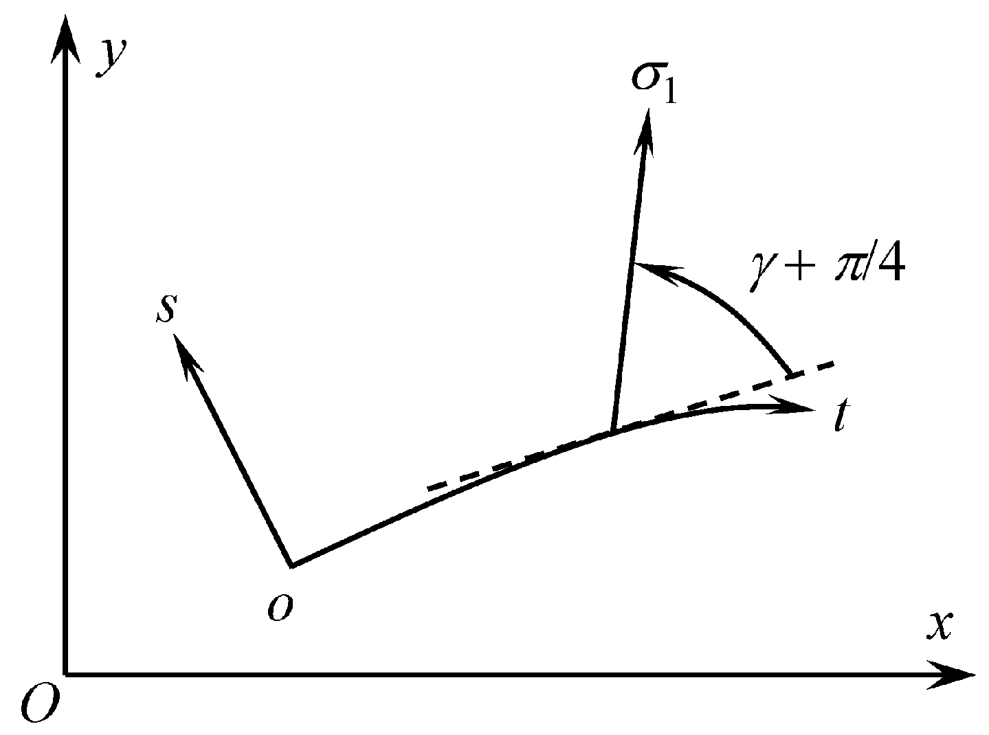
is introduced in planes of flow. This coordinate system is illustrated in
Figure 1, where
is the orientation of the principal stress
relative to the
direction, measured anticlockwise positive from the
direction. The
curve corresponding to
is given. The
lines are straight and orthogonal to this
curve. All other
curves are orthogonal to the
lines. It is always possible to introduce such a coordinate system in a vicinity of any smooth curve. It is also always possible to assume that the scale factor of the
lines is unity. Let
,
, and
be the stress components referred to the
coordinate system.
Then, the equilibrium equations are [
27]
Here
H is the scale factor of the
curves and the terms
and
are independent of stress derivatives. Let
,
, and
be the strain rate components referred to the
coordinate system. Then [
27],
Here
and
are the velocity components referred to the
coordinate system, and
and
are independent of these components and their derivatives.
One of the principal strain rates vanishes under plane strain conditions. Assume that
and that the direction of the principal stress
coincides with the
z-direction of the Cartesian coordinate system. Then, it is seen from (2) and (5) that
Combining the first of these equations and the identity
gives
. It is possible to assume, with no loss of generality, that
. Then,
and the second equation in (1) becomes
The transformation equations for stress component in a plane result in (
Figure 1)
Substituting (11) into (12) yields
where
and
. It is convenient to rewrite (6) and (7) as
The first two equations in (5) and (11) combine to give
or
Since the material is incompressible and the material model is coaxial, it is evident from (12) that
4. Characteristics and Characteristic Relations
Substituting (13) into (8) and using (14) one gets
One can choose the
coordinate system such that the principal direction corresponding to the principal stress
is tangent to a
curve at a point. Then,
(
Figure 1) at this point and the equations in (17) become
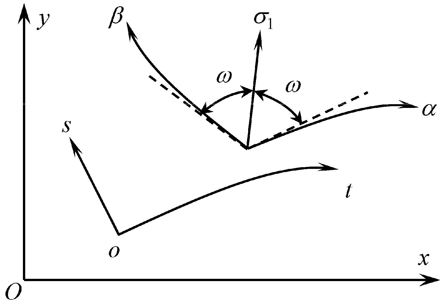
Then, the equation for stress characteristics is
The solution of this equation is
Here and in what follows, the upper and lower signs correspond to
and
characteristic curves, respectively (
Figure 2). It is evident from (14) and (20) that the system of equations is hyperbolic if
Henceforward, attention is concentrated on this regime. It is seen from (20) that the angle between the principal stress direction corresponding to
and each of the characteristic directions is
Since the orientation of characteristic curves has been determined, it is convenient for deriving the characteristic relations to choose the
coordinate system, such that one of the characteristic directions is tangent to the
curve at a point. Equation (17) is valid. However,
at the point in question. To derive the relation along
lines, one should put
. Then, Equation (17) becomes
Multiplying the first equation by
, the second by
, and summing gives the characteristic relation of the form:
Analogously, putting
in (17) leads to the characteristic relation along
lines of the form:
In Equations (24) and (25), and are elements of length along the and lines, respectively.
The velocity characteristics and corresponding characteristic relations are found from (9), (15), and (16). In particular, these equations combine to give
As before, one can choose the
coordinate system, such that the principal direction corresponding to the principal stress
is tangent to an
curve at a point. Then,
(
Figure 1) at this point and the equations in (26) become
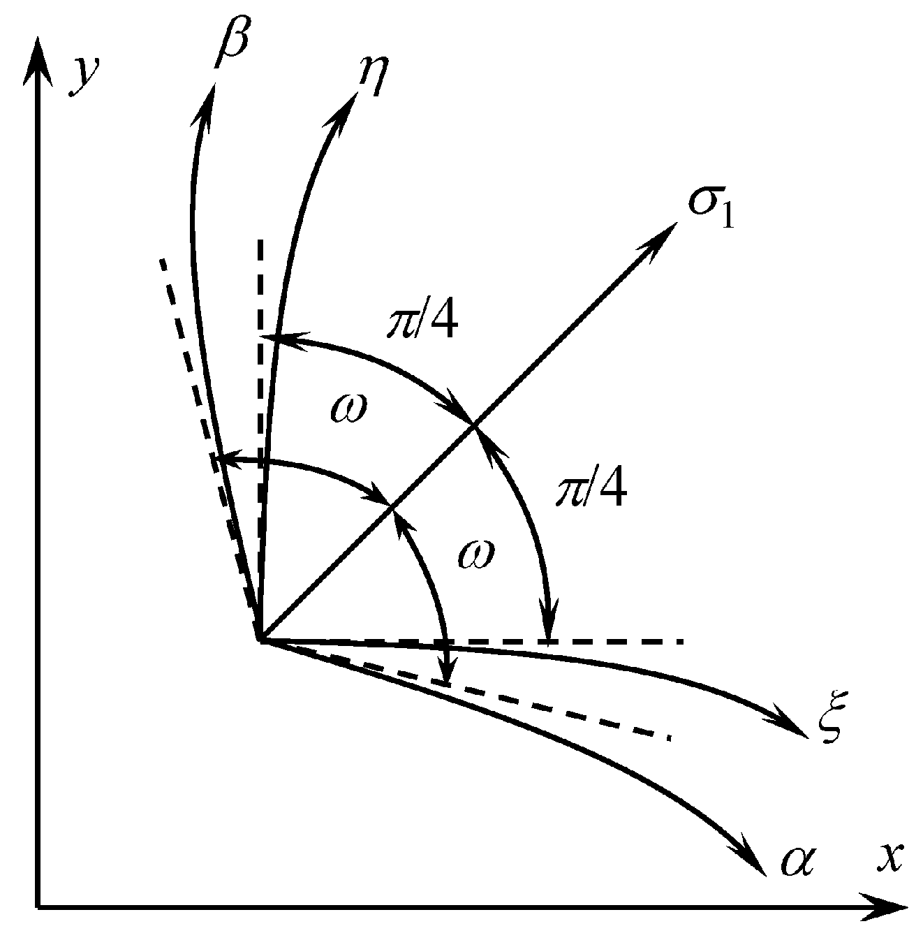
Then, the equation for velocity characteristics is
The solution of this equation is
Here and in what follows, the upper and lower signs correspond to
and
characteristic curves, respectively. It is evident from (29) that the angle between the principal stress direction corresponding to
and each of the characteristic directions is
. Equation (22) and condition (14) imply that
Therefore, the orientation of the characteristic lines is as shown in
Figure 3.
To derive the characteristic relations, it is convenient to choose the
coordinate system, such that one of the characteristic directions is tangent to the
curve at a point. Equation (26) is valid. However,
at the point in question. To derive the relation along
lines, one should put
. Then, Equation (26) becomes
The first equation is the characteristic relation along the
lines. This equation can be rewritten as
A similar relation is valid along the
lines. In particular,
In Equations (31) and (32), and are elements of length along the and lines, respectively. Additionally, and are the components of velocity referred to the characteristic coordinate system. Of course, in (31) and (32) depend on the geometry of each characteristic curve.
5. Asymptotic Behavior of Solutions near Envelopes of Characteristics
Consider the stress characteristics. Assume that the curve
coincides with an
characteristic curve or an envelope of
characteristics. Then,
on this line. In what follows, it is assumed that all stress and velocity components are bounded everywhere, all derivatives with respect to
s are bounded at
, and the solution is represented by Laurent series with respect to
s in the vicinity of the curve
. In this case, the variation of
with
s in the vicinity of the curve
is represented as
as
. In this equation,
is independent of
s and
is constant. Then,
as
. Multiplying the first equation in (17) by
, the second by
, summing, and using (34) gives
as
. Multiplying the first equation in (17) by
, the second by
, summing, and using (34) gives
as
.
If
and
at
then (35) coincides with (24) and; therefore, the curve
coincides with an
characteristic curve. To study the behavior of solutions near envelopes of characteristics, one has to assume that
as
. Then, it follows from (33) that
Equation (35) contains the product
. It is seen from (33) that the order of this product is
as
. None of the other terms involved in (35) may be of the same order, unless
. Therefore,
and
as
. It follows from this equation that the forth term in Equation (36) is of order
as
. To cancel this term, one has to assume that
as
. Here
and
are independent of
s.
Since
at
if
, it is evident from (26) that the derivatives
and
are bounded at
. If
then
as
[
8].
6. Conclusions
The constitutive behavior of some polymers at large strains is adequately described by pressure-dependent yield criteria and pressure-independent plastic potentials. The system of equations for plane strain deformation is hyperbolic if the condition (21) is satisfied. However, in contrast to many rigid plastic models [
11,
28,
29], the characteristic curves of stress and velocity equations do not coincide. This feature of the system of equations causes additional difficulties with the description of solution behavior near envelopes of characteristics. On the other hand, such descriptions are important for developing numerical codes because of possible singularities in stress and/or velocity fields.
It has been shown in the present paper that the stress field near an envelope of stress characteristics is singular in the sense that the derivative of stress components with respect to the normal to the envelope approaches infinity. The exact asymptotic representation of stress solutions is given by (40) and (41). On the other hand, all derivatives of velocity components are bounded unless
. In the latter case, the stress and velocity characteristics coincide as follows from (20), (22), and (29). This special case has been treated in [
8].
In the case of pressure-independent plasticity, the singularity in solution behavior may significantly affect the temperature field near the singular surface [
30]. This effect is due to the plastic work rate, which is involved in the heat conduction equation. The plastic work rate approaches infinity in the vicinity of characteristic envelopes together with the quadratic invariant of the strain-rate tensor and; therefore, results in a singular term in the heat conduction equation. In the case considered, it is difficult to expect the same result because the quadratic invariant of the strain-rate tensor is bounded everywhere.
The main result found is useful for developing numerical codes based on, for example, the extended finite element method [
31].


