1. Introduction
A battery management system is an important component of an electric vehicle especially in pure electric vehicles (PEV) where the battery is the only source of power. The battery applications for electric vehicles (EV), hybrid electric vehicle (HEV) and areas where batteries can be used as a primary source of energy have been widespread over the past few years due to the transition of internal combustion engine (ICE)-based automobile industries to EVs and HEVs [
1]. Use of renewable electricity resources in EVs and HEVs plays a significant role in the transition towards sustainable transportation [
2]. One of the major challenges faced by the current EV industry is the overall driving range, which is much lower compared to the ICE vehicles. Adding to the problem is a lack of a battery management system that can estimate and predict the actual remaining power of a battery i.e., to predict the residual driving range. Therefore preventing EVs from running out of charge or leaving the passengers stranded is the main concern [
3].
Thus, better control and management strategies for battery capacity are required in order to safeguard the performance and to extend the battery’s useful life. In order to predict the residual range of the electric vehicle, one of the parameters directly involved in its calculation is state of charge (SoC). SoC describes the battery’s remaining capacity status and is critically important for accurate measurement of EV battery state. SoC will give drivers an indication of available runtime and will also help to avoid some detrimental situations like overcharging or over-discharging which might reduce the useful lifespan of a power battery [
4]. Therefore, there is a need for a battery that has high energy density, has a long service life and, most of all, is environmental friendly. Automotive industry nowadays considers Li-ion batteries as the preferred choice over the conventional batteries like Ni-MH, Mi-Cd and lead acid batteries due to its high single cell voltage, high energy density and long service life [
4,
5]. As opposed to the conventional methods for measuring the remaining gas or fuel in a car, SoC cannot be measured directly with physical sensors because of the battery’s strong non-linear and time-variable system.
Several methods for estimating or measuring SoC have been proposed and reported [
6,
7,
8,
9,
10,
11,
12]. Each method has its own pros and cons. SoC estimation methods can mainly be divided into two main categories. The first category includes non-model based techniques that are based on the type of measured or estimated input variable. The discharge test, open circuit voltage (OCV) and ampere hour counting methods all fall under this category. The discharge test method is very time consuming and viable only under laboratory conditions though it is one of the most reliable methods. Contrary to the discharge test method, the OCV-based SoC estimation method is a promising technique that obtains SoC from the battery’s OCV-SoC relationship [
2]. The second category deals with different kinds of battery models in combination with several adaptive control algorithms.
Battery models can also be further classified into three main categories i.e., (1) a physical model that is designed for a specific battery factor (e.g., temperature model [
13] and cycle life model [
14]). However, one specific factor cannot describe the functioning and operation of the whole battery; (2) an electro-chemical model that captures the significant electrochemical processes of a battery through a complex mathematical equation and as a consequence makes the state estimation process difficult [
4,
15]; (3) an equivalent circuit model (ECM) captures the electrochemical physics of a battery using only electrical components, and generally includes an
nth order resistor-capacitor (RC) circuit with a series impedance factor, making it easy to incorporate into the system model of an electric vehicle with more precision and lower computational cost. However, according to [
16] higher
nth order RC circuit adds more non-linearity to the model, resulting in a more complex ECM.
Several adaptive control algorithms in combination with these battery models are used to estimate the states of a lithium ion battery. Different variants of Kalman filtering techniques are mostly used to estimate the SoC based on different battery models. The extended Kalman filter (EKF) was first used to estimate the SoC by Plett [
5] and Xiong et al. [
17,
18,
19] further improved it. However, Plett [
20] came up with unscented Kalman filter (UKF) idea to overcome the drawbacks of EKF i.e., the derivation of Jacobian matrix is very trivial making it highly unstable during linearization. However for systems with high non-linearity or with a non-Gaussian model the overall estimation performance of the Kalman filter family decreases drastically. Therefore, a particle filter (PF) as an alternative solution has been presented in order to cope with the highly non-linear/non-Gaussian models. PF is a probability-based estimator that can be utilized for SoC estimation dealing with both the Gaussian and non-Gaussian distributed noise models. PF utilizes the particles (weighted random samples) to approximate the posterior distribution sampled by Monte-Carlo methods [
21].
Besides system filtering theory, several other machine learning algorithms have been reported for SoC estimation [
22,
23,
24,
25] such as artificial neural networks (ANN), fuzzy logic based estimation and many others. These estimation methods offer good performance but are computationally intensive and may require complex processors that are too expensive to be used in a real-time automotive energy management system. Support vector machine (SVM)-based regression offers an alternative method for SoC estimation. Using the principle of Vapnik-Chervonenkis (VC) dimensional statistical learning theory (SLT) and structural risk minimization theory, SVM builds an optimized network structure with the right balance between the empirical error and VC confidence interval. Thus, it achieves a better generalization performance than ANN [
26]. However, the disadvantage is that they are dependent on the quality and quantity of the training data, which makes them computationally very expensive.
This paper adopts the least square method to identify the parameters of the lithium ion equivalent battery model and estimates SoC based on EKF, PF and UKF algorithms. The remainder of the paper is organized as follows.
Section 2 discusses the battery model selected for the experiment while
Section 3 briefly discusses the use of EKF, the application of Sequential Monte Carlo (SMO), i.e., PF and UKF, for Li ion battery SoC estimation based on the current integral method and the open-circuit voltage method, followed by the results and conclusion in
Section 4 and
Section 5, respectively.
2. Battery Modeling
A battery model describes the relationship between the battery factors and its running characteristics. There are a lot of definitions found in the literature for SoC. In this paper, we will use the following definition: the SoC of a battery is the ratio of the full capacity to the present maximum available capacity. According to the SoC definition [
27] it can be represented by Equation (1):
where
is the present SoC;
is the initial SoC value;
is the instantaneous load current (as assumed positive and negative for discharging and charging phase respectively) and η is the columbic efficiency, which is determined by the aging of the battery. In this paper we assume η = 1.
is the rated columbic capacity that differ from the battery’s rated capacity due to the aging effect.
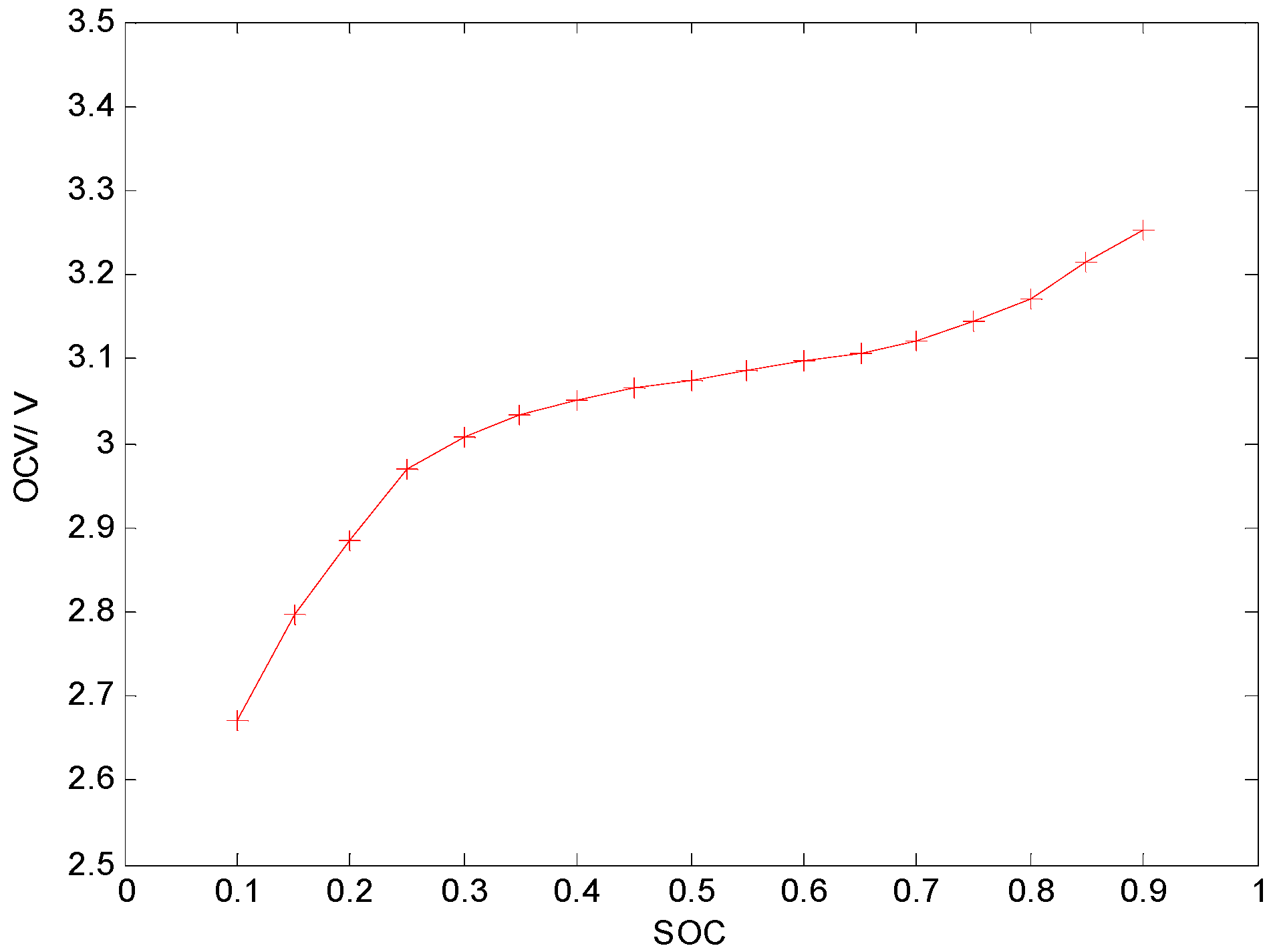
Figure 1 shows the open circuit voltage.
As the algorithm will be implemented into a digital system, transforming Equation (1) into a discrete form gives Equation (2):
where
n is the sampling step and
is the sampling period.
2.1. Battery Model
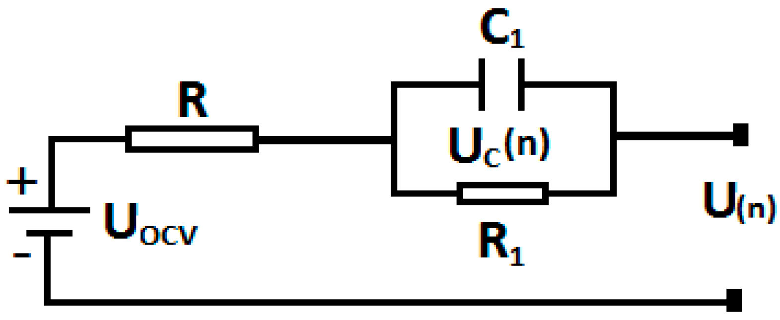
An ECM for Li ion battery with one OCV source and a parallel RC network was selected as shown in
Figure 2.
The source, parameterized as a non-linear function of the battery SoC and the OCV, is to describe the open circuit voltage characteristic at different SoC. Time-dependent polarization and diffusion effects of the cell are represented by the parallel ladder.
The state space equation of the battery circuit is presented in Equations (3) and (4).
In the above model, is the time constant of the RC network.is the sampling time and. and are assumed to be Gaussian noise.
2.2. Least Square Method
One of the most widely used method to find or estimate the numerical values of the parameters is least square method [
30]. It can also be used to fit a function to a set of data and to characterize the statistical properties of the estimates. The principle of the least square method is as follows: a set of
N pairs of observation {
} are used to find a function given the value of the dependent (
Y) from the values of an independent variable (
X). With one variable and a linear function, the prediction is given by Equation (5):
In Equation 5, a and b are two free parameters which specify the slope and intercept of the regression line respectively. The least square method defines the estimate of these parameters as the value which minimizes the sum of squares between the measurements and the model. This amounts to minimizing the expression:
where
stands for error which is the quantity to be minimized, and this is achieved using the standard technique property i.e., a quadratic formula reaches its minimum value when its derivatives vanishes. Taking the partial derivative of
with respect to a and b and setting them to zero gives the following set of equations:
To identify the parameters of the battery pack listed in
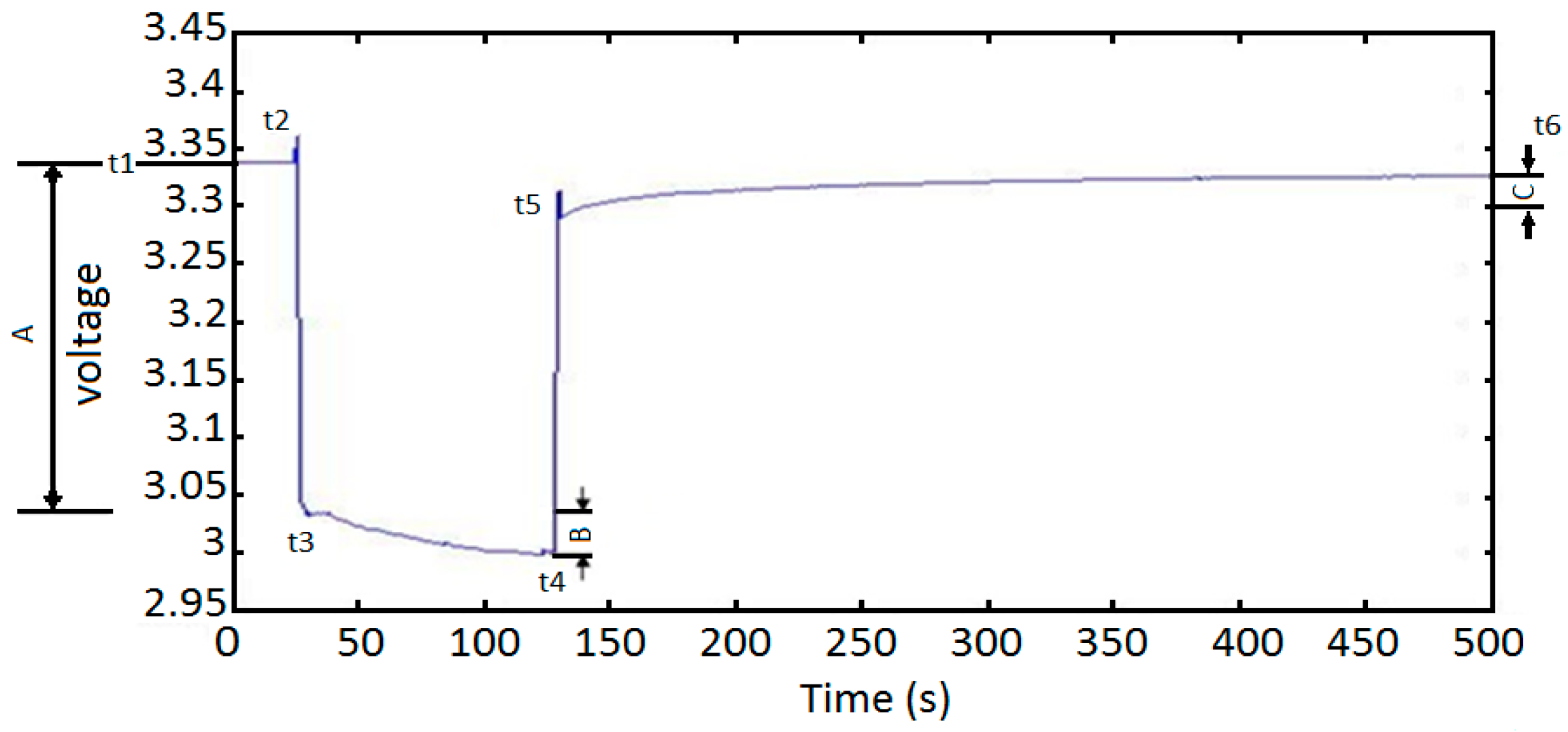
Table 1 during the discharging process, a constant current pulse is produced, which is constant for sometime, in order to identify the relevant parameters by varying the pulse current as shown in
Figure 3.
In this experiment, we obtained the parameters of the Thevenin battery model shown in
Figure 2 based on the least square method and the characteristic of the voltage response of the constant pulse-current discharge.
Figure 3 is the voltage response process of a 20 A constant pulse-current discharge. The parameter identification process is as follows: when the pulse-current is removed, the bus current
, and the terminal voltage of the battery becomes
until the polarized capacitor discharges gradually
.
Phase C in
Figure 3 shows the slow discharge reaction due to the capacitance
C1 of the RC circuit at the end of the discharge process until the voltage returns to normal. The zero input response of the RC circuit is
in which
is the time constant. Apply the least square method to obtain
.
Phase B in
Figure 3 consists of two parts. One part is the voltage drop of the terminal voltage which is caused by the pulse-current discharge. The second part is the voltage drop of the RC circuit. Thus we can easily get the voltage drop of the RC circuit
. The zero-state response of the RC circuit is
. By applying the least square method again, we can get the parameters
and
.
The ohmic resistance parameter
is obtained from voltage drop difference in phase A of the response process shown in
Figure 3.
Thus all the parameters of the battery ECM are obtained.
3. Battery SoC Estimation Approach
3.1. Extended Kalman Filter
EKF is a non-linear version of the Kalman filter as the non-linear function is Taylor expanded and the high order terms are ignored. A brief summary of EKF is given below:
| Summary of Conventional Non-Linear EKF |
| Non-linear state-space model |
|
|
| Definitions |
|
|
| , |
| Initialization |
|
|
| Computation |
| State estimate time: |
| Error covariance time: |
| Kalman gain matrix: |
| State estimate measurement: |
| Error covariance measurement: |
3.2. Unscented Kalman Filter
For non-linear systems, UKF uses numeric approximations rather than analytic approximations. First UKF chooses a set of sigma (σ) points then the mean and covariance of these points are used to match the priori random variable’s mean and covariance in every estimation step. A weighting constant is assigned to each σ point and the overall sum of all the weighting constants is equal to 1. As a result we get a set of transformed points after passing all the σ points through a non-linear function. Finally, the mean and covariance of the transformed points are used to update the posteriori mean and covariance. One of the major differences between UKF and EKF is the σ point calculation.
The process model is described in Equation (13):
The state vector , is a discrete process. andare the control vectors and process noise respectively.
The observation model is described in Equation (14):
Here
is the measurement noise. Including the noise in Equation (14) gives us the new state vector presented in Equation (15).
The process noise , and measurement noise are Gaussian random processes with zero mean.
• Choose σ points
The state vector
has dimension
M = 5, mean
and covariance
, then
. σ points with their weight factors are generated using Equation (16):
is the ith column of the matrix square root of . is the weighting and is the weighting constant of σ point mean and σ point convariance respectively. They are defined as , .is a scaling factor defined as . The spread of the σ points is represented by w. incorporates prior information and is the optimal value for the Gaussian ditributions. is either 0 or 3 − M.
• State estimate time update step:
T, Q and R are the variance matrix of the primitive state variable, process noise and the measurement noise respectively.
• State estimate time update
Rewrite the σ points through Equation (3). We will get 2
M + 1 σ points
,
i = 0, 1, …, 2
M. The mean and convariance of the state vector can be calculated using Equations (19) and (20):
• Output estimate
Propagating the σ points through the observation function given in Equation (4) results in Equation (21):
Then, using Equations (22) and (23) to calculate the mean and convariance of the estimated output:
• Estimator Kalman gain matrix
In order to calculate the Kalman gain, the covariance matrix must be calculated prior to it being used in Equation (24):
• State estimate measurement update
Finally, update the state vector using Equations (26) and (27):
3.3. Particle Filter as a Sequential Monte Carlo Method
For complex battery models with strong non-linearity PF can be utilized to perform the SoC estimation. PF is a Monte Carlo method (SMC) that integrates the Bayesian learning methods with sequential importance sampling (SIS) and re-sampling. PF approximates the posterior by a set of particles associated with weights without any assumption of its form. In Monte Carlo simulation for state estimation, the given state
will be estimated with the observation
. The given equation can be utilized to approximate the posterior using Equation (28):
(
i = 1, 2, …,
K) are the random samples drawn from the posterior distribution and estimate Equation (29) can be utilized to approximate any expectations:
Without directly sampling from the posterior density function we can sample from the proposal distribution
[
15], and we can derive Equation (30):
Here
is the normalized importance weight. Normalize the weight for each particle (i.e., sum to total that equals 1) using Equations (31) and (32):
Hence we can approximate the empirical estimate Equation (28) as the following posterior density function in Equation (33):
Assuming the Markov process for the state we get Equation (34):
Hence the optimal choice for the proposal distribution is presented in Equation (35):
PF for SoC Estimation
For SoC estimation PF works in two simple steps, i.e., predict and update. According to the previous discussion about PF review, PF-based Li ion battery SoC estimation algorithm is discussed below:
• Initialization.
Select the total number of particles
L and generate the initial particles by using Equation (36):
is the Gaussian distribution where is the initial guess and is the error covariance.
• State prediction.
Propagate the particles using the system process equation to predict a new set of particles.
• Weight calculation and normalization step (importance sampling).
After calculating the particles maximum likelihood using Equation (37), generate the weights according to Equation (38) and then normalize the weights (Equation (39):
• Re-sampling step.
After normalization of the weights, generate random and uniform samples with a residual re-sampling technique.
• Determine output estimate using Equation (40):
n is the estimated SoC using PF. Repeat Steps 2–5 for all n = 1, 2, …
4. Experimental Results and Discussion
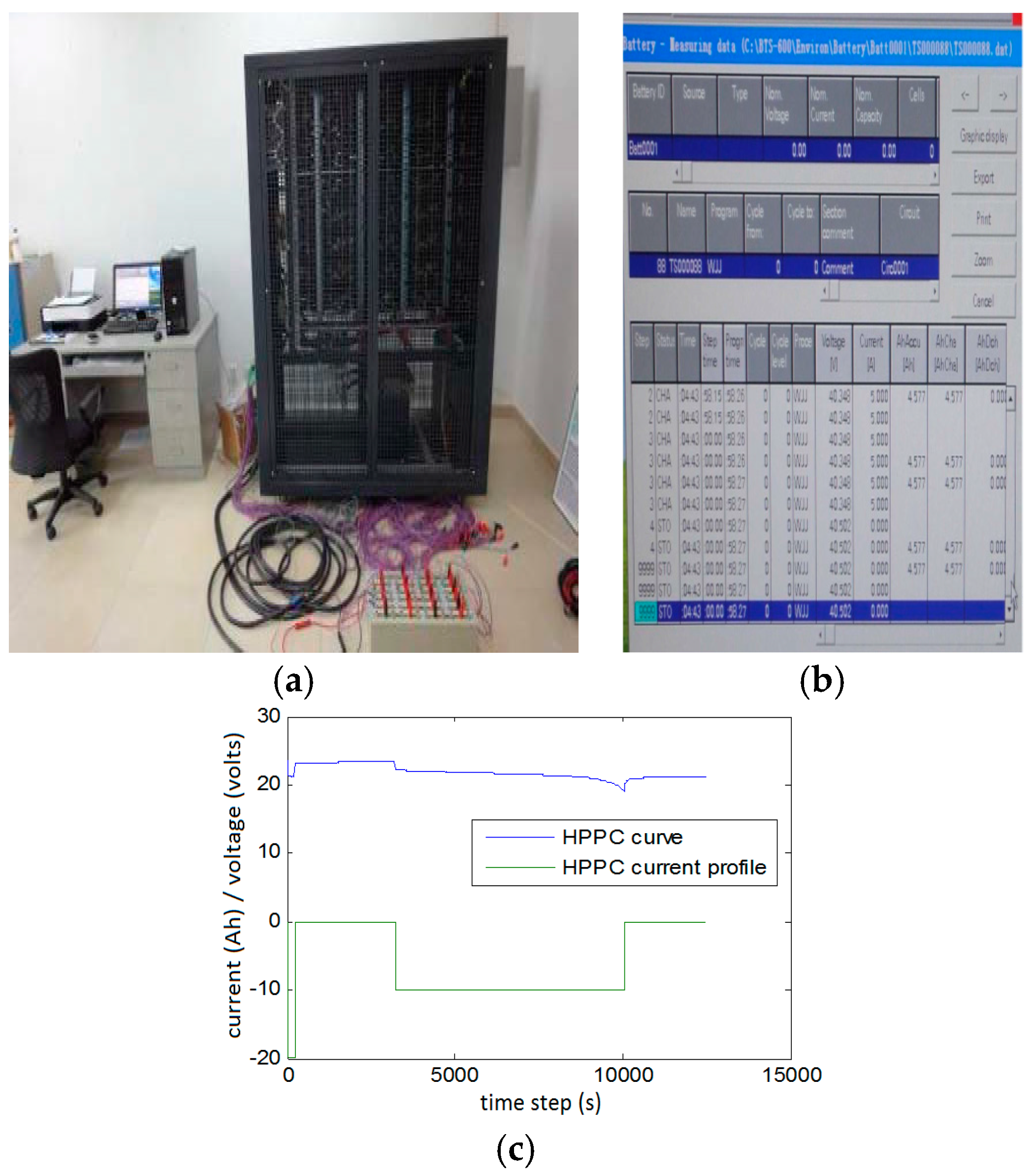
To validate the performance of EKF, UKF and PF, we used Shenzhen top band LiFePO
4 “3470160” cells (Shenzhen TOPBAND, Guangdong, China). The capacity of each single cell is 20 Ah, 3.2 V. The current and voltage information of the battery pack were recorded using a Digatron battery testing system (BTS) that has the capability to perform charge/discharge of multiple cells simultaneously to obtain charge-discharge capacity and energy. A host computer running the battery testing software recorded all the battery data including voltage, current, Ampere-hour (Ah) and temperature etc. Overall voltage and current sensors error were between 0.1% and 0.5% respectively. For noise cancelation, BTSs have a low pass filtering function. Battery SoC experimental data with the given sampled current and voltage was obtained by BTS management module’s designed algorithm shown in
Figure 4.
In practical situation a battery’s actual capacity is limited within the range of 90%–10% to protect it from any damage. 17 points from the voltage plateau area (from 2.6 V to 3.3 V) were chosen in order to get the constant current discharge curve of LiFePO
4 at 25 °C shown in
Figure 1.
From
Figure 1 it can be seen that the relationship between SoC and OCV is intrinsically non-linear. In order to describe this non-linear behavior we used 4 different kinds of OCV function [
31,
32,
33] to fit the OCV-SoC curve for SoC estimation given in
Table 2. The goodness-of-fit evaluation factors sum of squared error (SSE),
R2, adjusted
R2 and root mean square error (RMSE) are derived for each OCV function selected for SoC estimation.
Table 3 shows the experimental data for the identification of the parameters. All the parameters (
Table 4) were obtained from the OCV-SoC curve with their respective goodness of fit shown in
Table 5.
In
Table 2, “
s” represents the SoC of the battery and “
a1–
a4” is the coefficient obtained from the OCV-SoC curves.
Artificial Gaussian noise is added to the current (around 2% of the full range) in order to better evaluate the robustness of the SoC estimator in an environment close to a realistic automotive environment.
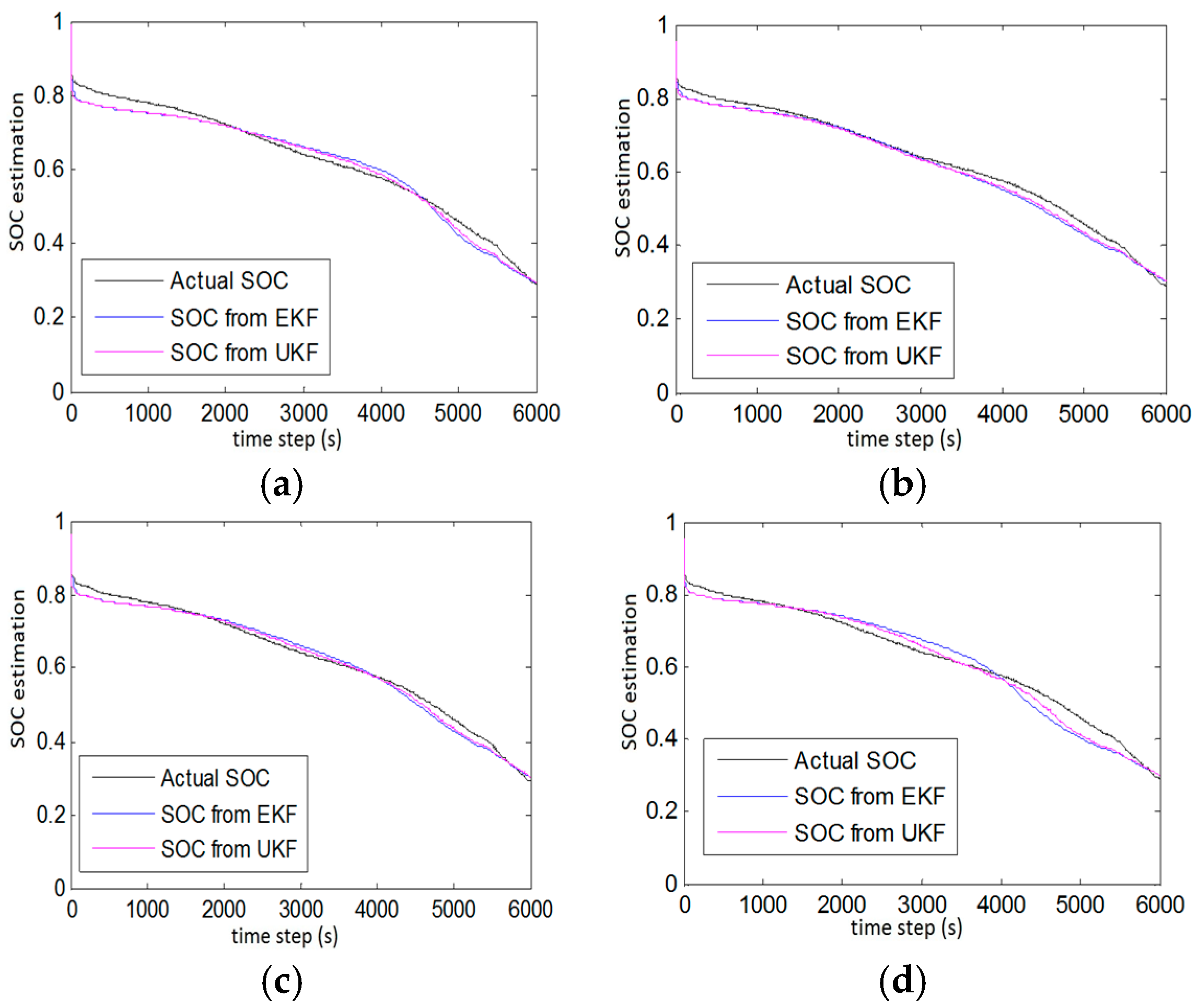
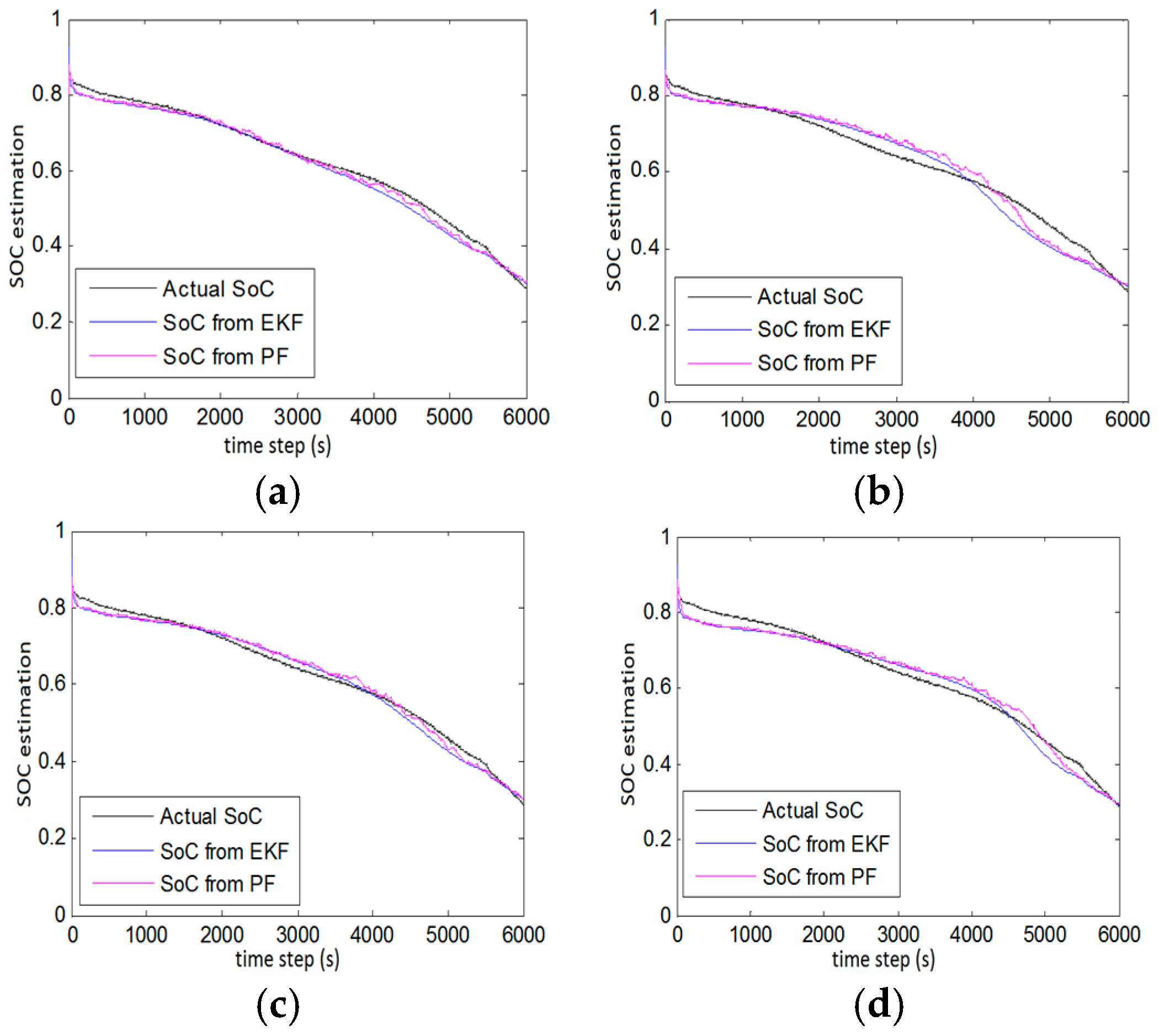
Figure 5 and
Figure 6 show the battery SoC estimation using the EKF, UKF and PF. During the experiments, 200 particles were chosen, but it was observed that the PF algorithm showed the same error even with 1000–2000 particles at the cost of high computational time.
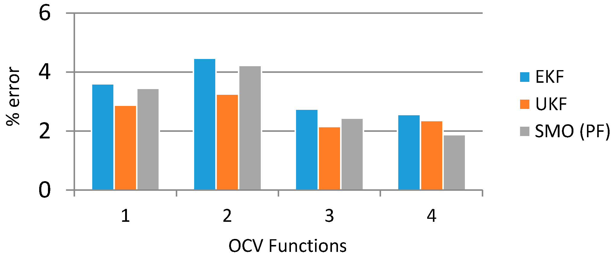
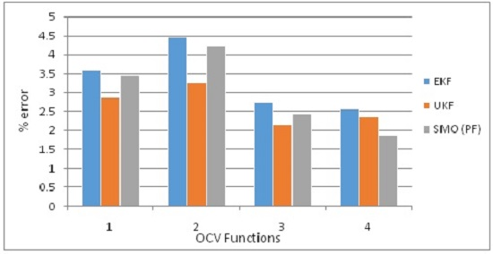
Choosing the right OCV function is the key to better estimating the SoC of the battery. Good estimation results were obtained when a logarithmic, exponential model with a polynomial exponent and high order polynomial functions were used. The overall performance of the logarithmic and high order polynomial functions is much better than that of exponential model with a polynomial OCV function (
Figure 7).
The higher the order of the polynomial function the better it fits as can be seen in
Figure 5b,c and
Figure 6a,c where a 4th order polynomial function produced better estimation results then a 3rd order polynomial function (
Table 5). However, the logarithmic function showed good estimation results with PF, but overall, UKF not only better tracked the actual SoC but also produced good estimation results.
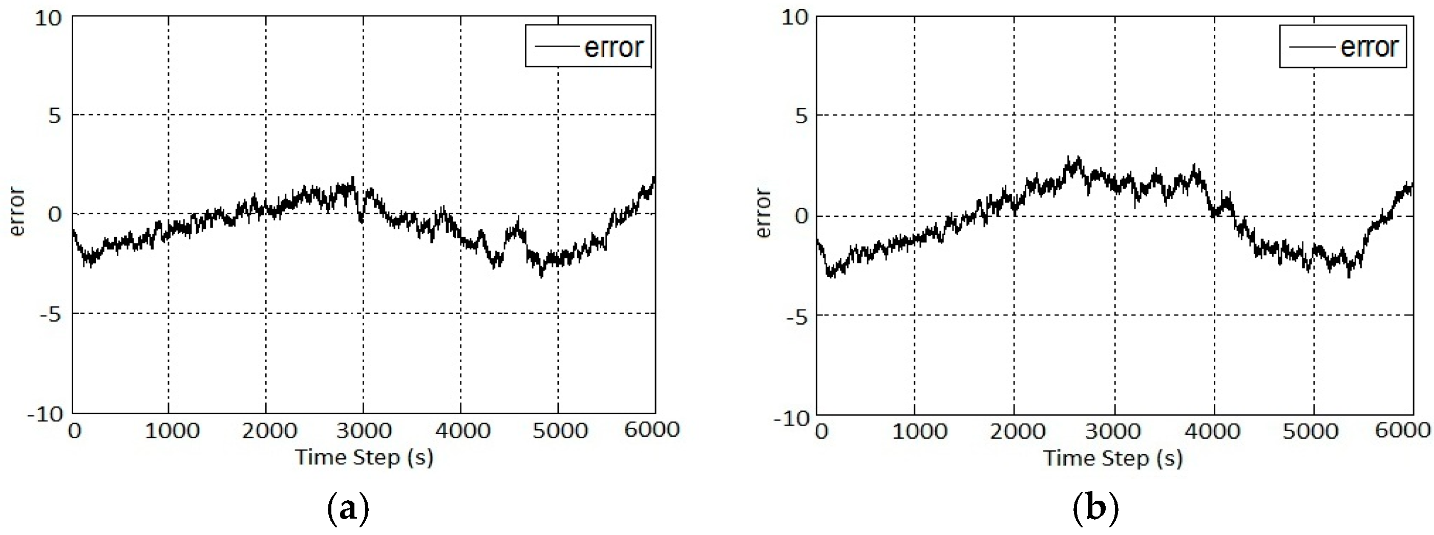
During the experiments it was noticed that all the SoC estimation methods, i.e., EKF, UKF and PF, exhibited a large error when the SoC is between 65% and 45%. The smoothness of the OCV-SoC curve is responsible for this estimation error.
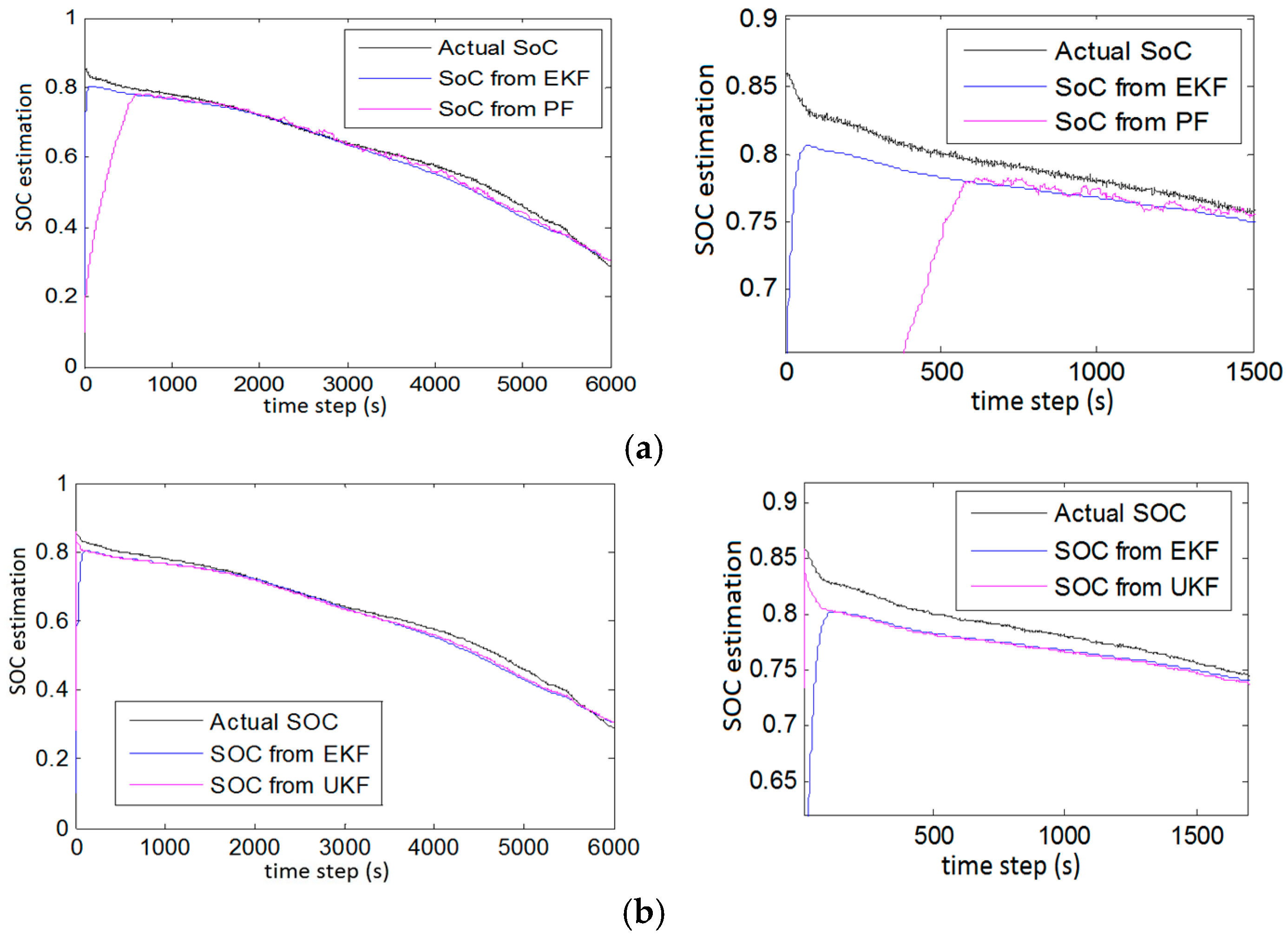
In
Figure 8a, it can be seen that when incorrect SoC is given, i.e., initial SoC = 0.1, PF was affected the most. Although it started tracking the actual SoC later, it took some time to recover the initialization error. However, UKF proved better than EKF though they also suffered from initialization error recovery as shown in
Figure 8b. Although both EKF and UKF were faster in terms of initialization error recovery but PF outperformed EKF when the battery model was affected by Gaussian noise or a higher order battery model is used which will add more non-linearity to the overall system shown in
Figure 9.
This experiment showed that both methods can be used as an alternative to the traditional EKF method in overcoming its weakness, i.e., higher order battery models, initialization error recovery and low accuracy. The overall percentage error is listed in
Table 6.


