1. Introduction
Software tools for thermodynamic modeling of internal combustion engines (ICEs) [
1,
2,
3,
4] have become indispensable for developing and optimizing the ICEs. Models that rely on engine maps constructed from steady-state measurements or models that use correction techniques to enhance the accuracy of the map-based modes in transient operation [
5] can be considered as an alternative to the thermodynamic engine models when modeling vehicle drive cycle performance. However, due to the higher level of prediction and the availability of all required sensor and actuator channels that are exchanged with the engine control unit, thermodynamic engine models are favored in the early stages of development where measurement data are not yet available. This applies to various model in the loop, software in the loop or hardware in the loop applications related to the development of engine controls and in applications where more detailed data on transients of gas path dynamics and engine torque (including cycle resolved torque) as well as on thermal responses of the components are required. Therefore, this paper focuses on the thermodynamic engine models.
Due to hardware performance constraints and due to computational time limitations, commercial thermodynamic engine simulation tools for modeling the complete internal combustion engine, including intake and exhaust manifolds, rely on 0D and 1D modeling approaches and do not incorporate three-dimensional (3D) modeling approaches, or just take advantage of using coupling to the 3D software to resolve phenomena in a specific selected component. Although the 0D and 1D models are based on a mechanistic basis, they incorporate many tuning parameters. Tuning parameters are employed due to the inability of the 0D and 1D models to fully capture 3D fluid flow and heat transfer phenomena, which are additionally coupled with mass transfer phenomena and chemical kinetics mechanisms during fuel injection, evaporation and the combustion phase. Tuning parameters in general include friction and heat transfer multipliers as well as combustion parameters. Tuning parameters have a clear physical interpretation and can, therefore, be adjusted within a meaningful range characteristic for particular phenomena. Adjusting of the tuning parameter to meet the accuracy threshold that is generally required in advanced projects (agreement of measured and simulated engine results should typically be in the range of 1% to 3%) is time-consuming and presents a considerable part of the work load of the whole project.
It has already been shown that optimization methods are suitable for determining optimized configurations of the components, e.g., manifold geometry [
6], valve lift profiles and timings [
7,
8,
9,
10,
11,
12], shape of the injection rate [
13], exhaust gas recirculation (EGR) rates and multiple injections [
14], injection timings [
15], constants of the heat transfer model [
16] and parameters of the combustion model [
17,
18,
19]. These analyses either use a calibrated ICE simulation model as a starting point for evaluation of the optimized configuration [
6,
7,
8,
9,
10,
11,
12] or tune a specific sub-model by optimization methods and compare simulation results to the measurement data [
17,
18,
19].
The authors of [
20] offer the automated calibration of combustion and heat transfer parameters in a cylinder (e.g., the radiation coefficient, the combustion terminal angle, the oil-drop breaking length, the rolling absorption rates before and after combustion, the rolling absorption rate after impaction, the early rolling fluctuation rate, the early rolling duration, the combustion speed and the flame retarding coefficient) of the ICE model in Reference [
2], using the advantages of a combination of two optimization algorithms, the ant colony and genetic algorithm, respectively. The methodology is focused on only three engine output results, e.g., power, brake specific fuel consumption and the turbocharger turbine inlet temperature at engine full-load steady-state operation. Additionally this methodology does not take into account potential calibration parameters (CBPs) of the intake, exhaust and EGR system which also influence the accuracy of the simulation results. Furthermore, differences between simulation and measurement results of the power and of the turbine inlet temperature in four of five engine speeds seems to still be high without any detailed information about the magnitude (e.g., in %).
The number of the tuning parameters required to calibrate the simulation model of the advanced turbocharged compression-ignited ICE with a variable turbine geometry and EGR system can vary in a range between 15 and 40. This might be inconvenient if only the optimization methods should be employed to calibrate the simulation model, since the effectiveness of the optimization techniques decreases with the increasing number of optimization parameters [
18,
21]. Furthermore, different searched calibration sets might be obtained for identical initial conditions after rerunning the optimization methods. This can be attributed to the relatively weak linear independence of the particular sets of CBPs and also to a large elongated space which consists of potentially several regions with very similar or even identical minimum values of the objective function. Weak linear independence of the tuning parameters can be identified and demonstrated also during manual calibration procedures. These trends were observed and analyzed by the authors during an attempt to calibrate 20 parameters of the entire ICE simulation model (ICESM) in one step, applying a widely used commercial optimization software tool package in Matlab
® [
22] for the model-based calibration (MBC Toolbox) by trying Multistart points gradient-based, Patternsearch and Genetic algorithms. Additionally, the required time for ICESM calibration using the optimization methods increases approximately exponentially with the number of tuning parameters, which imposes an additional limitation when applying a large number of tuning parameters characteristic of models of modern engines.
To efficiently address the issues encountered by the application of the optimization methods to calibrate a large number of tuning parameters that are characteristic of modern engines, an innovative method based on a combination of physics-based methods and optimization methods (denoted the Hybrid Calibration Method, HCM) is presented in this paper. In addition, to efficiently address issues imposed by the relatively weak linear independence of particular sets of CBPs, the proposed hybrid calibration method relies on a consistent division of the simulation model of the ICE into sub-systems. This division into sub-systems is based on the available measurement data, which provide well-defined boundaries of the sub-systems, from the system division and measurement validation point of view. The framework features a high level of generality to comply with various sets of available measurement data. The calibration process of the innovative HCM is thus performed in two steps. The goal of the first step is to tune parameters of the ICESM sub-systems applying physics-based approaches, while the objective of the second step is to perform calibration of a reduced number of the most dominating parameters in several loops by using entire the ICE simulation model together with an application of the optimization methods.
Division of the ICESM into feasible sub-systems enables a reduction of the total number of degrees of freedom of the entire ICESM, yielding better control over the calibration process and resulting in a faster calibration process and more accurate calibration results. Physics-based calibration of the suitable sub-systems makes possible an accurate and fast evaluation of the corresponding CBPs. This is preferably performed by the same code as used for model simulation, ensuring high level of consistency and a lower implementation demand as presented in this paper; however, the applicability of the method is not limited to such cases. Therefore, modular-based HCM enables fast and accurate calibration of ICESMs with an arbitrary number of CBPs.
2. Engine Simulation Model
HCM is applicable for any engine topology (ICESM), an arbitrary number of CBPs and various sets of available measurement data required for the calibration. In the presented analysis HCM will be demonstrated on the ICESM shown in
Figure 1. The ICESM is represented by a four-stroke, four-cylinder, 1.4 l turbocharged compression ignited engine with variable turbine geometry, high pressure-cooled EGR system and the cylinder compression ratio 17.5. The ICESM was developed in the commercial software tool package AVL CRUISE M™ [
4] and it enables the simulation of the thermodynamic process of an ICE covering the complete intake, exhaust and EGR system (air path) as well as cylinders including the engine block structure. In the demonstrated model, the air path is modeled with a combination of 0D and 1D elements based on a filling and emptying approach and it interacts with the crank angle-resolved 0D cylinders [
23,
24]. However, the applicability of the HCM is much more general and can also cover models featuring higher and lower levels of fidelity until it is possible to divide them into sub-systems (in the most general case it can also be applied to non-ICE related applications, however this lies outside of the scope of this paper). Application objectives of the ICESM in the presented work are high-fidelity-system-level simulations covering steady-state and hot transient operating conditions at arbitrary engine speed and load.
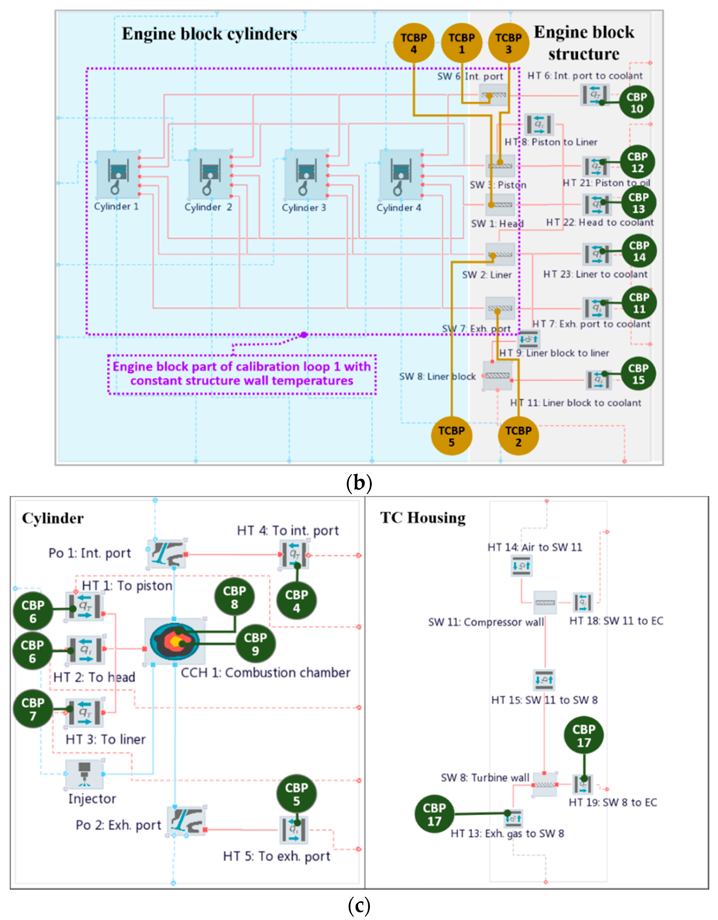
According to these objectives of the ICESM and according to the objectives of the paper (elaboration of the calibration method for system-level simulation models of ICEs), the paper focuses on the internal combustion engine simulation model, which interacts with its adjacent domains via the boundary conditions. The ICESM thus includes the engine cooling domain (
Figure 2a,b), which comprises: (1) convective heat transfer between the lumped solid walls of the engine block structure and the coolant or oil temperature boundary (e.g., HT 6: Int. port to coolant, HT 21: Piston to oil, …, HT 11: Liner block to coolant (
Figure 2b), (2) conductive heat transfer between the piston and liner, the liner and liner block and between the liner block and exhaust manifold (e.g., HT 8: Piston to Liner, …, HT 11: SW 9 Eng. block (
Figure 2a,b), and (3) coolant and oil temperature boundary (e.g., Amb 2: Coolant T, Amb 3: Oil T (
Figure 2a). The engine cooling domain is inherently a part of the engine. The engine cooling domain interacts with the cooling and lubrication circuit domain presented in [
25] via the heat flux between the engine block structure and the cooling as well as lubrication fluids. Therefore, the ICESM uses the coolant and oil temperature specified in the temperature boundaries as boundary conditions. Analogically to the cooling and lubrication circuit domain, the ambient air temperature represents a boundary condition of the intercooler and coolant of the EGR cooler represented by SW 4: IC coolant T and SW 11: EGR coolant T in
Figure 1. Ambient temperature, pressure and composition also represent boundary conditions of the engine air path (SB 1: Eng. inlet, SB 2: Eng. outlet in
Figure 1). In steady-state simulations, which will be the main focus of this paper as they provide a basis for a systematic analyses of the accuracy of the model, the engine model propels a brake (MC 1: ICE brake in
Figure 1), representing another boundary element that maintains engine speed and consumes the torque. In transient simulations that are presented in
Appendix C, the ICESM is propelled by the engine brake running in speed mode. Likewise, transient cold start functionality can be modeled if the ICESM is coupled to the model of the cooling and lubrication circuit as presented in [
25], whereas these simulations are outside of the scope of this paper.
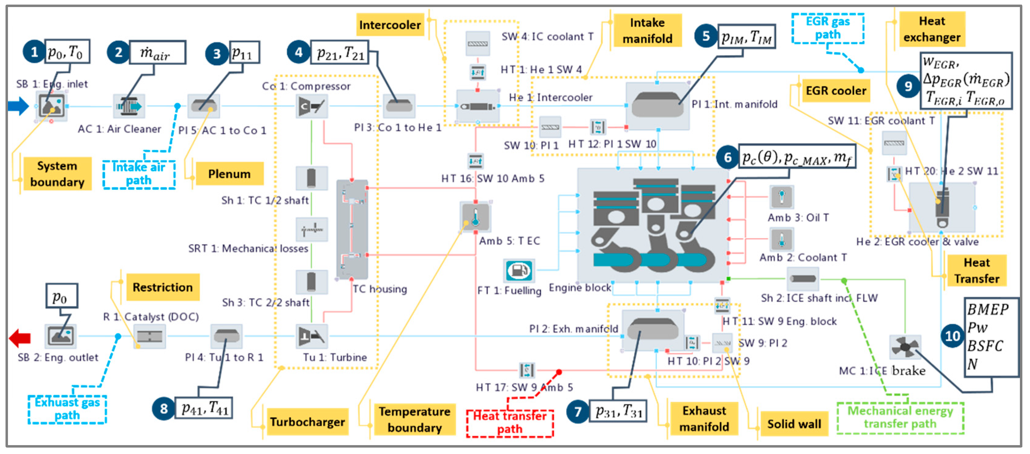
Figure 1 additionally presents available measurement data applied for the ICESM calibration and their positions (labeled positions 1, 2, …, 10) with respect to the sensor positions in the analyzed engine on the test bed, which represent a typical set of measured data in standard measurement investigations of a turbocharged engine. As mentioned in the Introduction, the HCM features a high level of generality and it is therefore able to comply with various sets of available measurement data. Therefore, the presented case used for demonstration of the applicability of the method should by no means be considered as the sole application case.
In
Figure 1, labeled quantities
,
denote the static pressure and temperature at a certain position, whereas subscript
i denotes: 0 is the ambient, 11 is the compressor inlet, 21 is the compressor outlet,
is the intake manifold, 31 is the exhaust manifold, 41 is the conditions at the turbine outlet,
is the EGR cooler inlet and
is the EGR cooler outlet conditions.
represents the air mass-flow,
is the injected fuel mass per cylinder per engine cycle,
is the cylinder pressure trace,
is the peak firing pressure,
is the EGR cooler pressure drop at the reference EGR mass-flow
,
is the EGR rate,
is the brake mean effective pressure,
is the brake power,
is the brake specific fuel consumption and
is the rotational speed of the ICE. In order to reach the target boost pressure (
in plenum Pl 3: Co to He 1) at a certain operating point (OP) a proportional-integral-derivative (PID) controller was applied in the ICESM to set the proper vane positions of the turbine. An additional PID controller was employed to control the target air mass-flow rate by the ICE part load operation by steering the EGR valve position. The engine friction mean effective pressure (FMEP) used in the ICESM as a two-dimensional (2D) map depending on the engine speed and load (BMEP) was extracted from the similar (type and size) measured engine.
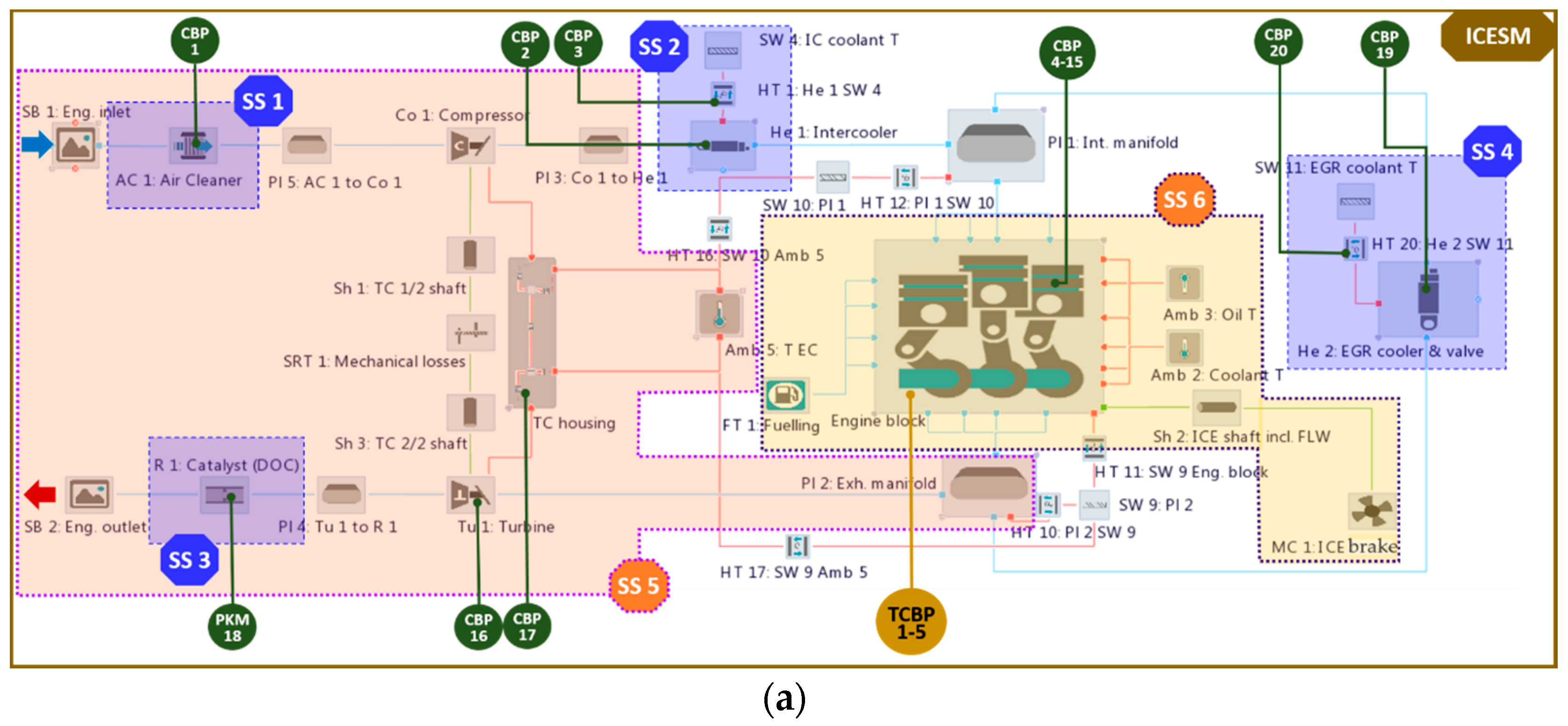
Based on the available measurement data (
Figure 1), the ICESM is divided into sub-systems presented in
Figure 2a marked with SS 1, SS 2, …, SS 6. The employed division complies with the availability of a typical set of measurement data in standard measurement investigations of the turbocharged engine. However, for other potentially available sets of measurement data, the division should be adapted accordingly. The sub-systems in
Figure 2a represent: the air cleaner (SS 1), intercooler (SS 2), catalyst (SS 3), EGR cooler (SS 4), turbocharger with part of the intake and complete exhaust system (SS 5) and cylinder (SS 6).
Figure 2b,c show a detailed view of the engine block, cylinder and turbocharger housing, respectively.
Additionally,
Figure 2 shows CBPs that are marked with green and golden-yellow circles. CBPs in green circles labeled with CBP # denote all the ICESM calibration parameters to be tuned. CBPs are classified according to the means of their calibration, i.e., physical or optimization based, which is described in detail in
Section 4.3. This classification is indicated with superscripts 1–4 in
Table 1.
Additionally, CBPs are divided into global CBPs (denoted with superscript 5) that are characterized by the fact that they feature a single constant value, which means that they are not operating point-dependent, and operating point-specific CBPs. For points that are not calibrated, operating point-specific CBPs are determined by linear interpolation between the values in the operating points that were subjected to CBP determination. Temporal CBPs comprise CBPs of the components representing the boundaries of the particular ICESM domain, which is described in detail in
Section 4.2. They are subjected to calibration only in the particular loop which covers the domain including temporal CBPs. CBPs in golden-yellow circles labeled with TCBP # represent CBPs to be temporally tuned in the particular loop of the entire ICESM. The meaning of the particular parameter and its data range is listed in
Table 1. Quantity
in
Table 1 denotes the engine coolant temperature.
4. Calibration Method
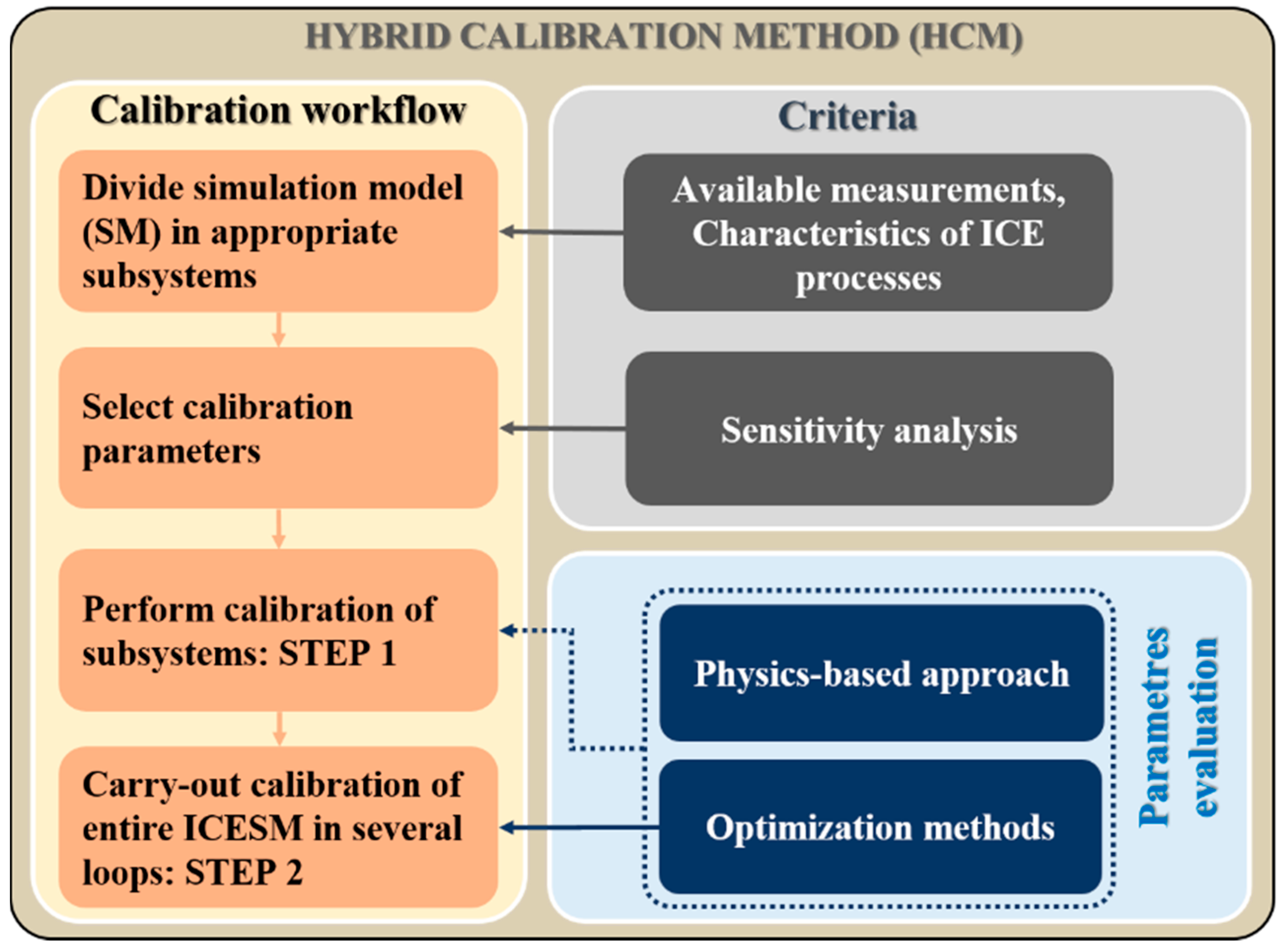
The basic calibration workflow, criteria of CBP selection and approaches to evaluate CBPs in the framework of the proposed HCM are presented in
Figure 4. The workflow consists of: the division of the ICESM into feasible sub-systems, the selection of the influencing CBPs, the calibration procedures of the sub-systems, and finally the calibration of the entire ICESM in several loops. In
Figure 4, STEP 1 represents the calibration of the ICESM sub-systems with physics-based approaches or optimization methods whereas STEP 2 is the calibration of the entire ICESM applying optimization methods.
The proposed innovative workflow was developed with the objective to comply with or to solve the following challenges of the ICESM calibration: coping with a large number of CBPs and consequently long computational time, issues encountered due to a potential weak linear independence between CBPs, and inherent potential multiple solutions as well as lower accuracy of the simulation results.
Division of the ICESM into sub-systems enables: (1) evaluation of some CBPs by a physics-based approach, which (2) reduces the number of degrees of freedom of the calibration procedure of the entire ICESM, and (3) increases the stability and accuracy of the calibration method. Physics-based approaches enable much faster evaluation of the target CBPs (no need for DoE execution, response function creation and searching parameters with an optimization algorithm) and an accurate evaluation of CBPs. Potential measurement errors outside of the expected error tolerances might also be detected.
A lower number of CBPs (degrees of freedom) which are consequently subjected to the calibration of the entire ICESM using the optimization methods yields the following advantages: enables better controlled convergence of the merit function to a global minimum; reduces the potential possibility for encountering issues due to the weak linear independence between CBPs; and requires a smaller design matrix and consequently less time is needed for the DoE simulations, response model (functions) generation, and finally for the parameter search with an optimization algorithm (
Section 3.2 and
Section 3.3). Additionally, better-fitting quality of the response models characterized by the factors
and
might also be achieved [
22,
34,
35]. The latter influences the accuracy of determined CBPs and consequently the simulation results. Carrying out the calibration of the entire ICESM in several loops offers an additional option to keep lower numbers of CBPs in one optimization round. A lower number of CBPs does not completely exclude the possibility for weak linear independence between CBPs which might result in multiple solutions. However, a lower number of CBPs enables easier and faster handling of this issue by narrowing intervals of inequality constraints and therefore the repetition of the optimization process as elaborated in
Section 4.5.4. In summary, HCM enables faster and more accurate calibration of the ICESM with an arbitrary number of CBPs in comparison with procedures based on the optimization methods only (e.g., Reference [
20]).
4.1. Division of the ICESM into Sub-Systems
Division into sub-systems is based on characteristics of the ICE processes in the observed sub-systems (e.g., pressure drop, heat transfer, high pressure phase within cylinder, etc.) and the available measurement data, which provide well-defined (from the system division and measurement validation point of view) boundaries of the sub-systems (
Figure 2). This is the first step to reduce the number of CBPs that are calibrated by the optimization methods.
As the number of the CBPs that remain for calibration by the optimization methods might still be too large, an additional division of the entire ICESM can be performed based on the division of the entire ICESM into domains, e.g., the engine domain (typically the main object of interest), cooling and lubrication as well as the underhood (ambient) domain. These domains always interact at the solid wall that features much longer characteristic times compared to the integration time steps of the model, thus providing an appropriate boundary for the domain decoupling. In addition, the engine calibration is initially performed for steady-state operation and thus it is possible to set plausible temperature values for the lumped solid walls. Therefore, it is possible to reduce the number of CBPs that are calibrated in the first calibration loop as shown in
Figure 2b, which improves stability as well as robustness of the optimization method. The remaining CBPs of the non-engine domains can therefore be calibrated in the second calibration loop, helping to achieve the objectives of the HCM.
It can also be mentioned that for steady-state simulation, CBPs of the engine domain only (calibrated in the first calibration loop) are usually sufficient, whereas to obtain accurate transient results CBPs of other domains are needed as they influence the time-dependent boundary conditions of the engine domain as shown in
Figure 2b.
4.2. Selection of the Calibration Parameters
Objectives of the selection procedure of CBPs are to identify parameters which significantly influence a variety of target simulation results depending on the change of a certain CBP, and additionally to define the lower and upper bound of each CBP. Therefore, it is proposed to perform the sensitivity analysis of all potential CBPs which cannot be determined by physics-based approaches to provide the basis for later selection of the influencing CBPs. Sensitivity analysis is thus generally performed for CBPs that are included in the governing equations of the applied ICESM (
Section 3) and that influence observed simulation quantities, e.g., the typical set of measurement data presented in
Figure 1.
Different approaches are proposed for sensitivity analysis [
41]. For the applied ICESM, the final set of CBPs shown in
Figure 2 and listed in
Table 1 was determined based on the sensitivity analysis using response models (
Section 3.2) according to [
22]. Bounds of the CBPs were defined based on the previous experiences with ICE simulations in [
4]. Responses models were generated from DoE data representing relative differences between the simulation results of the initial ICESM which was the subject of the later calibration and measurements (Equation (34)) for the quantities listed in
Table 2 (e.g.,
).
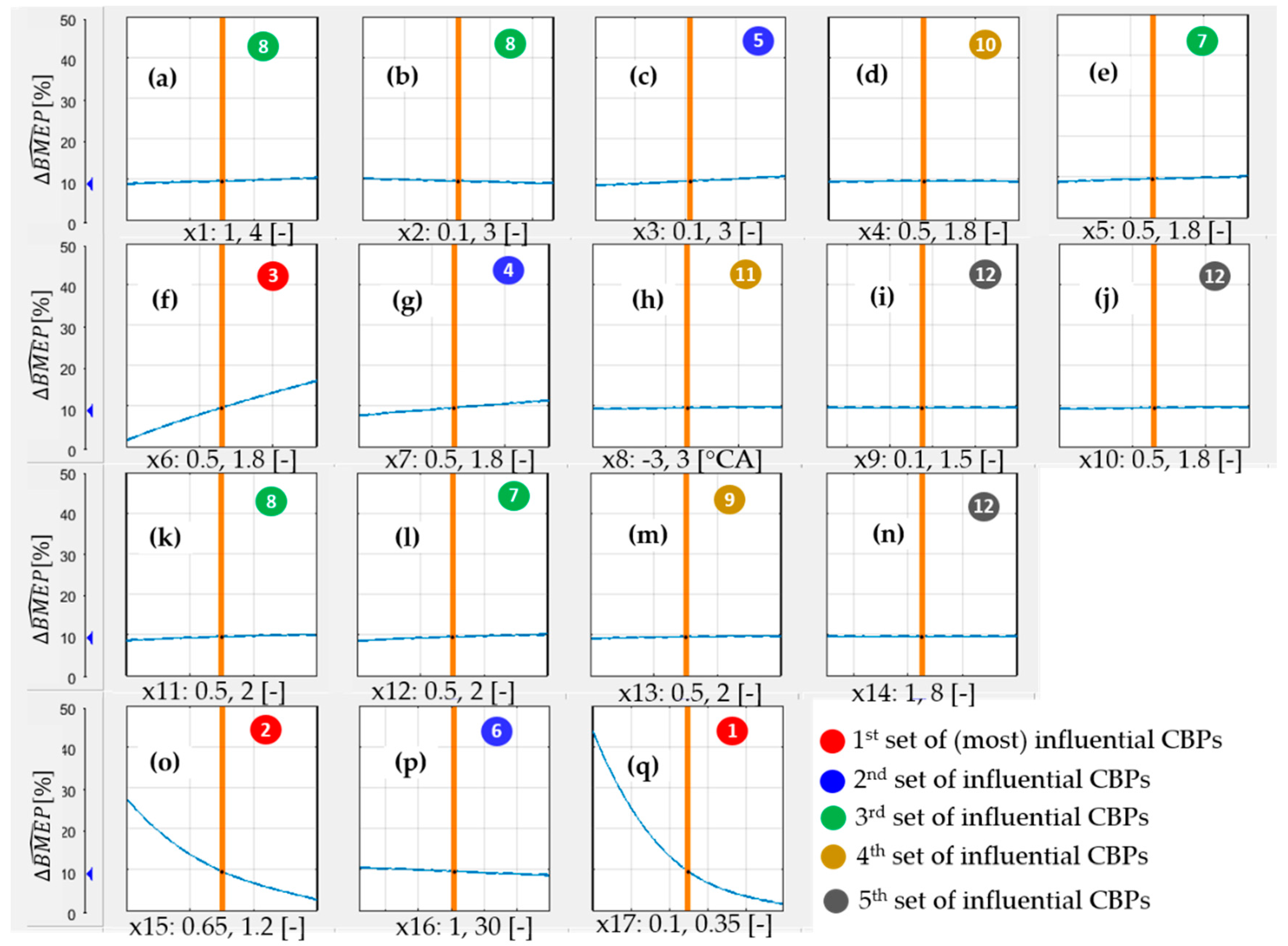
Sensitivity analysis was performed at minimum and maximum engine speed (e.g., 1000 rpm and 3800 rpm) at engine full-load and steady-state operation. Ranking and selection of the most influential parameters was finally carried out; it depended on the magnitude of the rate of change of a certain quantity (
,
,
,
,
,
,
,
,
,
and
) for the given interval of the single calibration parameter as shown in
Figure 5. For illustration purposes,
Figure 5 also includes CBPs which were evaluated by physics-based approaches (except the combustion characteristics in the cylinder described in
Section 4.4.2), whereas (as stated above) they are not included in the proposed workflow. It should be noted that
Figure 5 demonstrates only 1 of 11 analyzed quantities during the sensitivity analysis.
If a certain CBP showed an evidently higher influence on the single analyzed quantity, only it was selected (criteria for selection of CBPs was the magnitude of the rate of change >3% on the entire interval of the particular CBP, e.g., from the comparison x17 in
Figure 5q vs. x13 in
Figure 5m only x17 would be selected). The latter turned out to be the case (especially for CBPs in the air path) influencing the heat transfer, the pressure drop and the pressure in the sub-systems SS 1, …, SS 5 (
Figure 2a). Therefore, this confirms the plausibility of the evaluation of certain CBPs by a physics-based approach as explained in
Section 4.4. The influence of certain calibration parameters generally changes with the engine speed. CBPs feature a similar magnitude of the rate of change of the particular observed simulation quantity and indicate very similar trends at different operating points can be characterized as global CBPs (e.g., CBPs of the sets 4 and 5 in
Figure 5).
4.3. Classification of Calibration Parameters
After the division of the ICESM into sub-systems and a sensitivity analysis, classification of CBPs in the following groups can be performed:
CBPs determined by the physics-based approaches (
Figure 4).
CBPs determined by the optimization methods (
Figure 4), which can be further divided into:
- 2a.
CBPs characterized by the dominant influences of a single CBP on only one observed simulation quantity excluding those of item 1.
- 2b.
CBPs related to the engine domain excluding those of item 1 and 2a.
- 2c.
CBPs related to a non-engine domain excluding those of item 1, 2a and 2b.
It should be noted that the above classification clearly divides parameters into different groups, whereas in the calibration with the optimization methods it is also possible to optimize the various parameters of items 1 and 2 jointly in a single optimization loop as indicated below.
4.4. Physics-Based Calibration of the Sub-Systems
Physics-based approaches represent the first part of STEP 1 in the workflow of the HCM presented in
Figure 4. They rely on the same governing equations presented in
Section 3.1 as used in the ICESM. The most efficient approach is to use inverted equations of the same code used for the ICESM simulation to evaluate the CBPs of the sub-systems with lower complexity and thus a smaller number of CBPs, e.g., single components such as air cleaner (SS 1), intercooler (SS 2), catalyst (SS 3), EGR cooler (SS 4) and engine block (SS 6), marked in
Figure 2a.
4.4.1. Air Cleaner, Intercooler, Catalyst and Exhaust Gas Recirculation Cooler (SS 1–4)
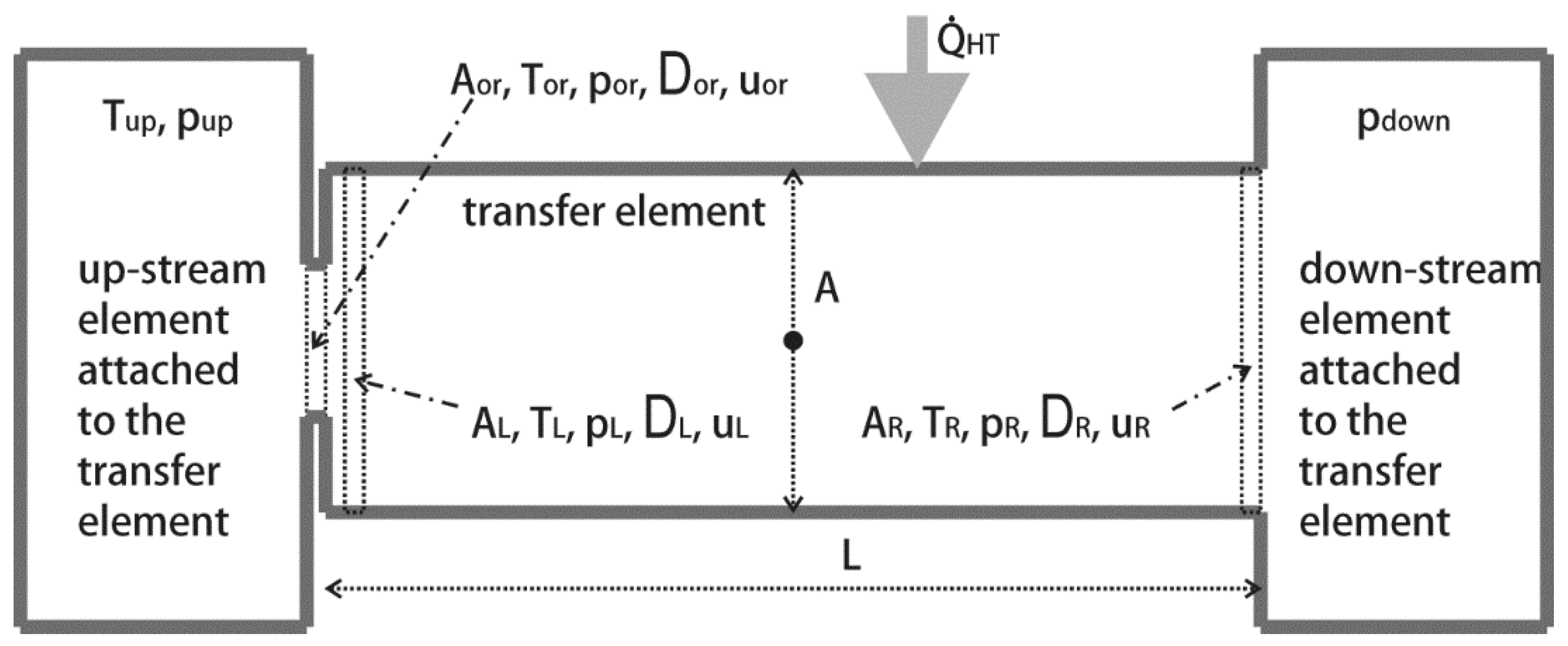
A transfer element with a finite length (
Section 3.1.9) was employed for the air cleaner, intercooler and EGR cooler modeling and a transfer element (
Section 3.1.8) was employed for the catalyst. Therefore, governing Equations (13)–(22) were employed for deriving appropriate CBPs, respectively.
FrMp was identified as a CBP of the air cleaner, intercooler and EGR cooler for the pressure drop calibration according to Equation (20), whereas the orifice flow coefficient (
) was identified for the catalyst according to Equation (13). In addition,
HTMp was selected as a CBP for tuning of the temperature difference across the intercooler and EGR cooler according to Equation (19). A flowchart of the evaluation procedure of the CBPs is presented in
Figure 6, covering the required input data (step s1) and workflow of the CBPs’ evaluation (step s2). Further,
and
were considered to calculate the pressure function
according to Equation (17) in [
29] (p. 2998), respectively.
4.4.2. Combustion Model (SS 6)
Sub-system SS 6 represents a high pressure phase of the in-cylinder process between the intake valve closure (IVC) and the exhaust valve opening (EVO). The objective of introducing SS 6 is to evaluate the rate of heat release (ROHR) in the engine cylinder (
Table 1) with the physics-based approach, applying Equation (9) together with other the cylinder balance equations outlined in
Section 3.1.5. Again, inverted equations of the same code are efficiently applied to evaluate ROHR, as was the case in the present study where the specialized software tool [
17] was applied. Evaluated ROHRs were later used in a map of tables [
26] as functions of the engine speed and load (injected fuel mass) in the applied ICESM. A high pressure phase can be employed also to determine CBPs other than ROHR traces, for example parameters of the Vibe combustion model, e.g., [
17].
Required input data for the piston, head, and cylinder liner wall temperature that ensure a sufficient accuracy of the evaluated ROHR are known to experienced users or they can be taken from the measurements of a similar engine type and displacement. However, the applied solid wall temperatures for ROHR evaluation might differ from the ones that finally took place in the employed ICESM. Therefore, the evaluated ROHR might include a small error resulting from the wall heat losses calculation (Equations (9) and (12)) which could consequently influence the BMEP. According to the author’s experience, this error is relatively small when an error interval of the employed wall temperatures is within 80 °C. Alternatively, it is also possible to perform a refinement calculation of the ROHR after the required input temperatures are calibrated by the HCM, afterwards repeating STEP 2 for the entire ICESM calibration (
Figure 4).
4.5. Evaluation of the Calibration Parameters with Optimization Methods
Application of the optimization methods is applied to sub-systems in which CBPs cannot be determined analytically and for the entire ICESM calibration (items 2a–c in
Section 4.3). Two approaches are proposed in the framework of application for optimization techniques:
Direct search of CBPs in a closed loop with the simulation model and searching algorithm based on simple control logic (e.g., bisection method or application of the PID controller elements [
26]).
Selection of the suitable optimization procedure is determined by two criteria: (1) whether the CBP dominantly influences only a single or several observed simulation quantities as discussed in
Section 4.2. and (2) the number of CBPs.
Generally RSM-based optimization methods can be applied for any type of CBP determination in a single loop or more loops, i.e., the CBPs listed in items 2a–c of
Section 4.3. However, it is beneficial to apply a direct search procedure for CBPs that are characterized by the dominant influences of a single CBP on only one observed simulation quantity (item 2a in
Section 4.3). This is done to determine the values of these CBPs or to obtain good starting values for their further optimization by the RSM, which improves robustness and reduces computational times of the RSM-based optimization. A direct search procedure is thus part of STEP 1 of the HCM as demonstrated in
Section 4.5.1. It should also be noted that the number of CBPs for the direct search procedure should not be too large to ensure the convergence stability of the applied simulation model. This condition is generally fulfilled as indicated in
Section 4.5.1, whereas if there are too many CBPs that could be calibrated by the direct search procedure then the RSM-based optimization approach is proposed. It should be emphasized that the direct search method is also much faster than RSM-based optimization because it does not require carrying out DoE simulations.
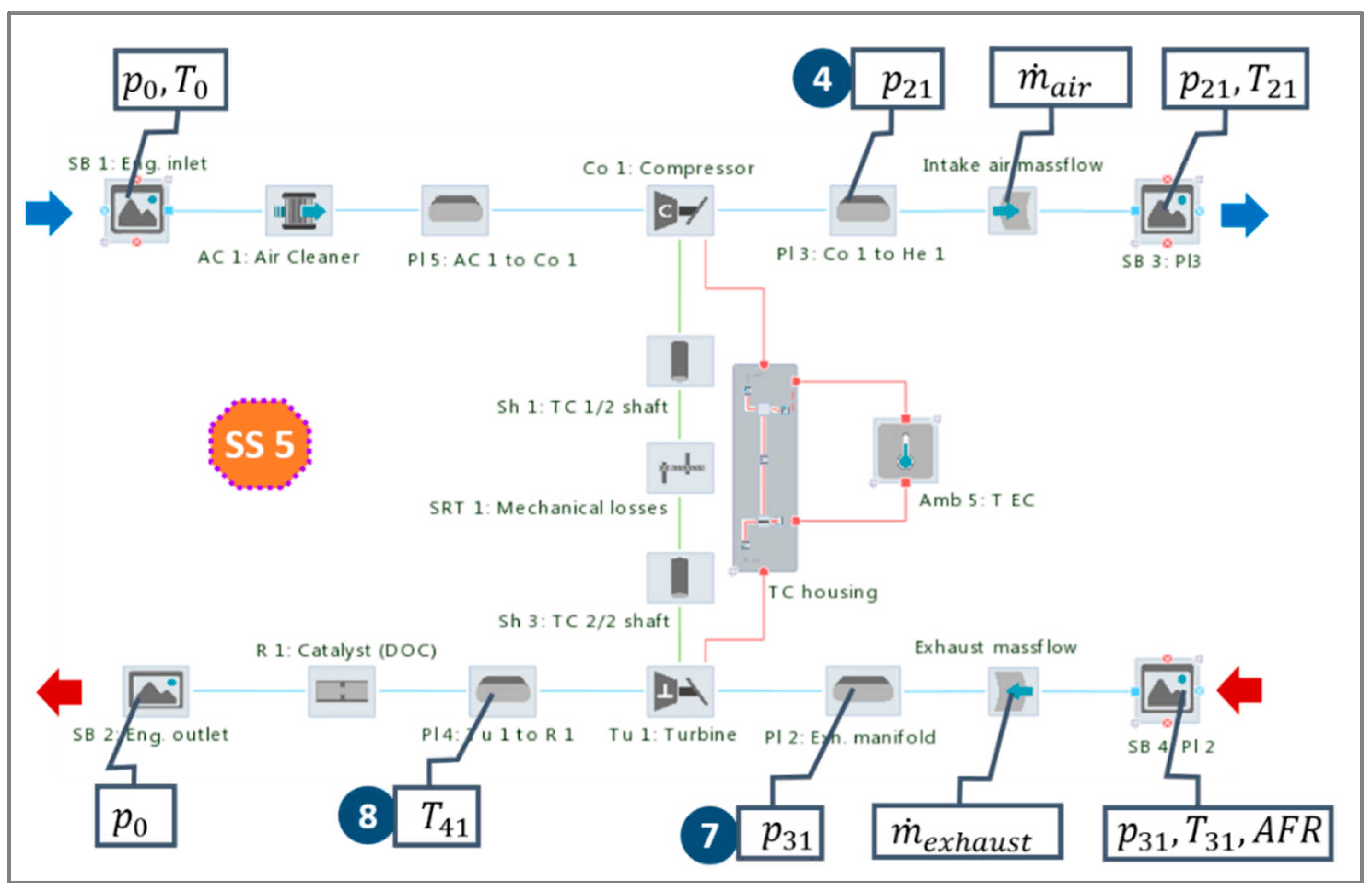
4.5.1. Calibration of the Turbocharger (SS 5)
The turbocharger sub-system (
Figure 7) represents the illustrative example for the application of the direct search optimization approach for CBP evaluation subjected to STEP 1 of the HCM (
Figure 4). The applied searching algorithm is based on a simple control logic realized by PID controller elements in a closed loop within the simulation model of the sub-system. Two target CBPs, the turbine
(Equation (3)) and the turbine efficiency correction factor (
Section 3.1.10), which are the dominant influences on individual observed simulation quantities, the turbine outlet temperature
and exhaust manifold pressure
, respectively, are determined. Besides the intuitive reasoning based on the analyses of the governing equations (Equations (23) and (24)), this fact is also confirmed by the sensitivity analysis (
Section 4.2). In addition to the turbine
and the turbine efficiency correction factor, the PID controller is also considered in the SS 5 simulation model for steering the turbine vane positions depending on the target compressor outlet pressure (
Section 2).
The SS 5 simulation model in
Figure 7 is inherently based on the mean value air path [
23,
26] due to the employed cycle-averaged measurement data for the boundary conditions. However, in the entire ICESM a highly pulsating flow is taking place [
23,
26] which can finally result in slightly different CBPs due to different flow conditions through the turbocharger [
23,
26]. Therefore, CBPs evaluated during the SS 5 calibration provide good starting values for the entire ICESM calibration (
Section 4.5.4) and additionally ensure better stability of the calibration of the entire ICESM. This represents an example of how CBPs from item 2a in
Section 4.3 can first be calibrated by the direct search procedure and can later be included in the RSM-based optimization.
Similarly to the SS 5 simulation model presented here, other topologies relating to the engine turbocharging, i.e., single-stage electrically assisted or two-stage ones, can be pre-calibrated in a similar way by using the direct search optimization approach as the number of CBPs is sufficiently small to allow for convergence stability of the applied simulation model for these topologies. This is determined by the fact that in the case of the direct search optimization approach, the authors experienced stable ICSEM behavior with up to six employed CBPs.
4.5.2. Calibration of the Entire ICESM
In this section, the term entire ICESM will be used as the entire engine model is always subjected to the RSM-based optimization methods. However, this does not necessarily mean that all remaining CBPs (this term will be used for the CBPs that are not subjected to STEP 1) are optimized simultaneously. If the number of the remaining CBPs for optimization is sufficiently small, optimization can be performed in a single loop comprising all remaining CBPs and, if required, selected CBPs that were subjected to optimization in STEP 1 can also be added to this optimization. As this is generally not the case for modern complex engine topologies due to the large number of CBPs, a multi-loop approach is applied in the HCM. This latter approach will be analyzed here to present the proposed optimization framework in a most general manner as simplification of the method in the case of a small number of CBPs is relatively straightforward. If the number of CBPs for the simultaneous optimization of all CBPs in a single loop is too large, the optimization is performed in multiple calibration loops, where the number of calibration loops is determined by the following criteria:
Number of the remaining CBPs.
Type of the remaining CBPs.
Strength of influence of the CBPs of different calibration loops or calibration STEPs on the merit function.
The number of selected remaining CBPs for one calibration loop depends on the proposed maximum number of the CBPs which still allow for an efficient utilization of the optimization methods. Simultaneous application of all CBPs should be theoretically possible in one loop. However, according to the authors’ experiences (similar findings were also presented in [
18]) based on the required computing time and coping with the weak linear independence between CBPs for the analyzed ICESM, efficient utilization of the optimization methods based on RSM is possible up to eight or 10 CBPs.
Considering this limitation on the maximum number of CBPs, calibration loops are formed based on classification of CBPs (
Section 4.3). Generally, CBPs of the engine domain (item 2b in
Section 4.3) are subjected to the first calibration loop and those of the non-engine domain (item 2c in
Section 4.3) are subjected to the second calibration loop.
As all CBPs are not calibrated in a single calibration loop if the number of CBPs is large and, as fitting quality of the response models is in general better if a smaller number of CBPs is applied for response model generation, a third calibration loop is introduced if the number of CBPs is larger and if remaining CBPs are not calibrated in a single calibration loop. This third calibration loop is introduced with the objective to more accurately determine the reduced number of CBPs with the most significant influence on the merit function (Equation (31)). This is reasoned by the fact that the model that enters calibration loop 3 already features well-defined values of CBPs and by the fact that the accuracy of determined CBPs is dependent on the fitting quality of the response models of the merit function and constraints featured by the factors
and
(
Section 3.2), which in general improves with the reduced number of CBPs. Therefore, CBPs with a prevailing influence on the magnitude of the merit function (Equations (31) and (32)) are selected for calibration in the third calibration loop.
4.5.3. Response Surface Methodology-Based Calibration Approach
The calibration workflow applying RSM-based optimization (
Section 3.2 and
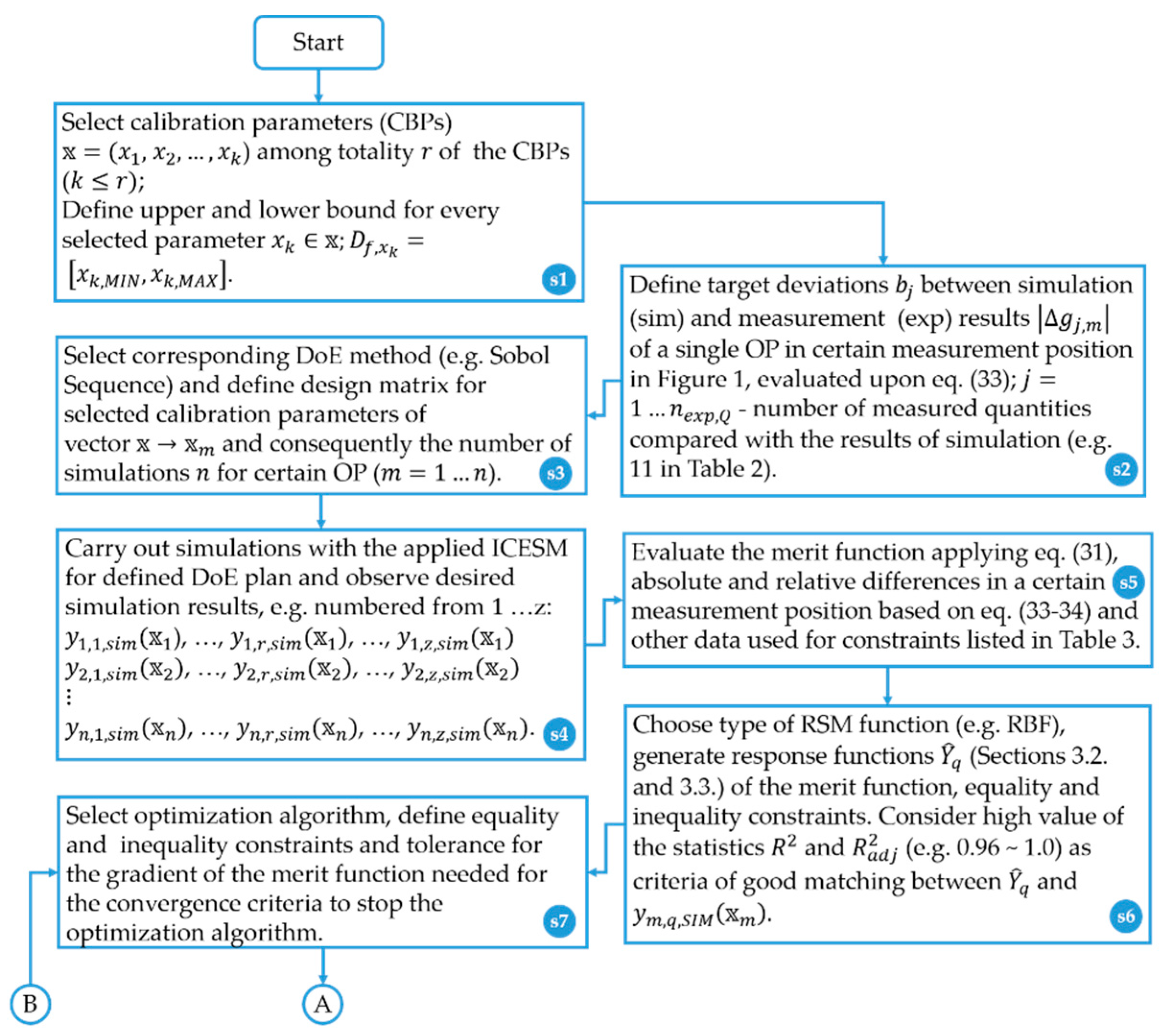
Section 3.3) was carried out according to the flowchart presented in
Figure A1 and
Figure A2 (
Appendix A). The flowchart corresponds to one calibration loop and consists of the steps labeled s1–s16. Step s1 comprised the selection of CBPs represented with the variables vector
and the specification of the bounds denoted by the
for each of the CBPs (
Table 1). During step s2 the target differences (
) between the results of simulation and the measurement for the quantities listed in
Table 2 were defined with the initial value of 3%. Step s3 comprises the creation of a design matrix for the selected CBPs from step s1 applying the Sobol Sequence DoE method as presented in
Section 3.2. Simulations with the employed design matrix data in the applied ICESM (
Figure 1) were performed in the simulation environment AVL CRUISE M™ [
4] (step s4). Step s5 requires data evaluation for the generation of the response models of the: (1) merit function; (2) constraints; and (3) absolute and (4) relative differences between the results of simulations and measurements (Equations (31)–(34) in
Section 3.3). Data were evaluated based on the results obtained in step s4. Data needed for inequality constraints 1–9 listed in
Table 3 were calculated based on Equation (33). In step s6 the response models of the merit function, the equality and the inequity constraints (
Section 3.3) listed in
Table 3, were generated by applying the Radial Basis Function as presented in
Section 3.2.
Steps s7–s9 comprised the execution of RSM-based optimizations using a gradient-based Sequential Quadratic Programming algorithm as presented in
Section 3.2. The objective of the optimization process was aimed at finding a minimum of the merit function (dependent on the applied CBPs represented by the variables vector
) for the employed equality and inequality constraints listed in
Table 3. Values of
defined in step s2 were initially employed for the target values of inequality constraints 1–9 in
Table 3. If it appeared that no solution was found with the initial values of the applied inequality constraints, their values were gradually increased until a single solution was found. However, an opposite trend can also appear when the optimization process converges to multiple solutions. In the latter case, convergence to the single solution was achieved by gradually decreasing the values of the inequality constraints 1–9 in
Table 3. Occurrence of both possible circumstances depends on the actual absolute differences between the results of the performed DoE simulations (step s4) and measurements (Equation (33)) used for the response model generation of the inequality constraints 1–9 in
Table 3 (step s6). Therefore, it is proposed to take the median value of a range of the actual absolute differences of the particular inequality constraint (e.g., 1–9 in
Table 3) for the initial target value of the same particular inequality constraint. A smaller median value of the actual absolute differences generally demands a smaller target value of the particular inequality constraint and vice versa.
Steps s10–s16 were continued after optimizations were finished for all engine operating points that were subjected to the performed calibration loop. Values of the global CBPs (
Section 2,
Section 4.2 and
Table 1) were determined in step s10 according to Equation (35). If the latter took place, this was followed by the repetition of the optimizations (s7–s11) for all engine operating points with the applied values of the global CBPs in the variables vector denoted as
(s10–s12).
Steps s13–s14 were followed after the optimizations were finished (s7–s12) and consisted of simulations with the applied ICESM and verification of the simulation results. Simulation results were obtained by the performed simulations with the employed optimized CBPs (s7–s12) in the applied ICESM. Verification of the simulation results with the measurements (
Section 2) was based on the comparison of the absolute differences (Equation (33)) and the values of
defined in step s2. If a sufficient agreement was achieved, the calibration process was ended; otherwise, it was continued with step s15.
4.5.4. Calibration Loops of the Employed ICESM
For illustrative purposes the calibration process will be demonstrated in this section to additionally explain the applied method and, in particular, the methodology of calibration loops on a real example of the applied ICESM presented in
Figure 1 and
Figure 2. CBPs in all calibration loops were determined with applied RSM-based optimizations according to the steps described in
Section 4.5.3.
For the analyzed ICESM, the number of remaining CBPs is 13 (
Table 1). As this number exceeded the number of CBPs proposed for one calibration loop according to the criteria in
Section 4.5.2, multi-loop calibration was performed. CBPs that correspond to the engine domain (item 2b in
Section 4.3) were calibrated in calibration loop 1; CBPs of the non-engine, i.e., cooling, domain (item 2c in
Section 4.3) were calibrated in calibration loop 2, whereas calibration loop 3 covered fine-tuning of two CBPs from calibration loop 2, which predominantly influence the merit function (
Section 4.5.2). Additionally, selected CBPs determined during calibration STEP 1 (
Figure 4) were applied in the RSM-based optimizations.
Calibration loop 1 covered CBPs of the engine domain and, additionally, one CBP (turbine efficiency correction factor) from SS 5 (
Table 1) with the most significant influence on the merit function identified during the sensitivity analysis (
Section 4.2). Global CBPs were determined by averaging CBPs characterized as global of all calibrated engine speeds after finished optimizations (
Section 2, and
Section 4.5.2 and
Table 1). By considering the values of global CBPs in variables vector, optimizations were repeated according to steps s12 and s7–s14 (
Figure A1 and
Figure A2). In calibration loop 1 it was also assumed: (1) a default value for the
HTMp of the convective heat transfer between the gas and the wall of the cylinder head and the wall of piston; (2) a constant wall temperature of the intake port defined depending on the coolant temperature by considering the relationship
, and (3) dependency of the cylinder head temperature on the piston temperature by considering the relationship
. The latter two applied assumptions were made based on the description presented in
Section 4.4.2.
Calibration loop 2 comprised CBPs of the cooling domain and two CBPs from SS 5 (the turbine efficiency correction factor and the turbine
HTMp). The turbine efficiency correction factor also showed the most significant influence on the merit function in calibration loop 1 (
Table 1), identified during the sensitivity analysis (
Section 4.2). The turbine
HTMp fixed values determined by the SS 5 calibration were used in calibration loop 1, due to the upper limit of eight of the total employed CBPs. However, the SS 5 featured different flow conditions (
Section 4.5.1) compared to the entire ICESM. Therefore, the turbine
HTMp was included in calibration loop 2.
As presented in
Section 4.5.3, calibration loop 3 aims at fine-tuning two CBPs with the most significant influence on the merit function. These two CBPs were identified during the sensitivity analysis (
Section 4.2) and, in the analyzed case, comprise the start of combustion offset and the turbine efficiency correction factor (
Table 1). The start of combustion offset significantly influences the peak cylinder pressure whereas the turbine efficiency correction factor influences the exhaust manifold pressure.
4.6. Calibration Method Summary
The HCM presented in this work represents a methodological background for the calibration procedure of the ICESM, which is intended to be implemented in an ICE modeling tool to support automatic execution the entire HCM workflow, where the user will be guided by the graphical user interface. This workflow comprises: (1) automated division of ICESM into sub-systems based on checking measuring points via the pre-prepared graphical user interface (GUI) functionality in the elements of the ICESM (
Section 4.1); (2) automated reading of the corresponding measurement data from the reference file using element-specific identification; (3) automated physical-based evaluation of CBPs in sub-systems (
Section 4.4) applying inverted equations of the same code as that used for ICESM simulation; (4) automated update of the evaluated CBPs by the physical-based evaluation in the corresponding elements; (5) automated execution of the sensitivity analysis (
Section 4.2); (6) automated classification of the CBPs (
Section 4.3), the proposed number of calibration loops and the assignment of CBPs to a calibration loop; (7) possibility for the user to change the number of calibration loops and CBP assignments to a particular calibration loop; (8) automated execution of optimization methods (
Section 4.5); and (9) verification of the simulated results with the measurement data and error analysis.
5. Results and Discussion
Results are presented for the ICESM shown in
Figure 1 and cover four, six or 13 full-load and six part-load operating points. The ICESM comprised, in total, 13 full-load and six part-load operating points. This section will focus on steady-state results as they provide a basis for analysis of the accuracy of the model, which was calibrated against steady-state data. Comparison of the measured and simulated data (presented in
Appendix B) thus provides the basis for the systematic analysis of the proposed calibration methodology. To confirm the prediction capability of the calibrated ICESM in transient operating conditions as well,
Appendix C presents the results of the hot transient operating conditions of the ICESM coupled with the engine brake running in speed mode.
5.1. Comparison of Different Approaches to Determine the Calibration Parameters
In this section, three different approaches to determine the calibration parameters (CBPs) of the applied ICESM are compared to highlight their characteristics and applicability. These approaches comprise:
Comparison of the simulation results in
Figure 8 and
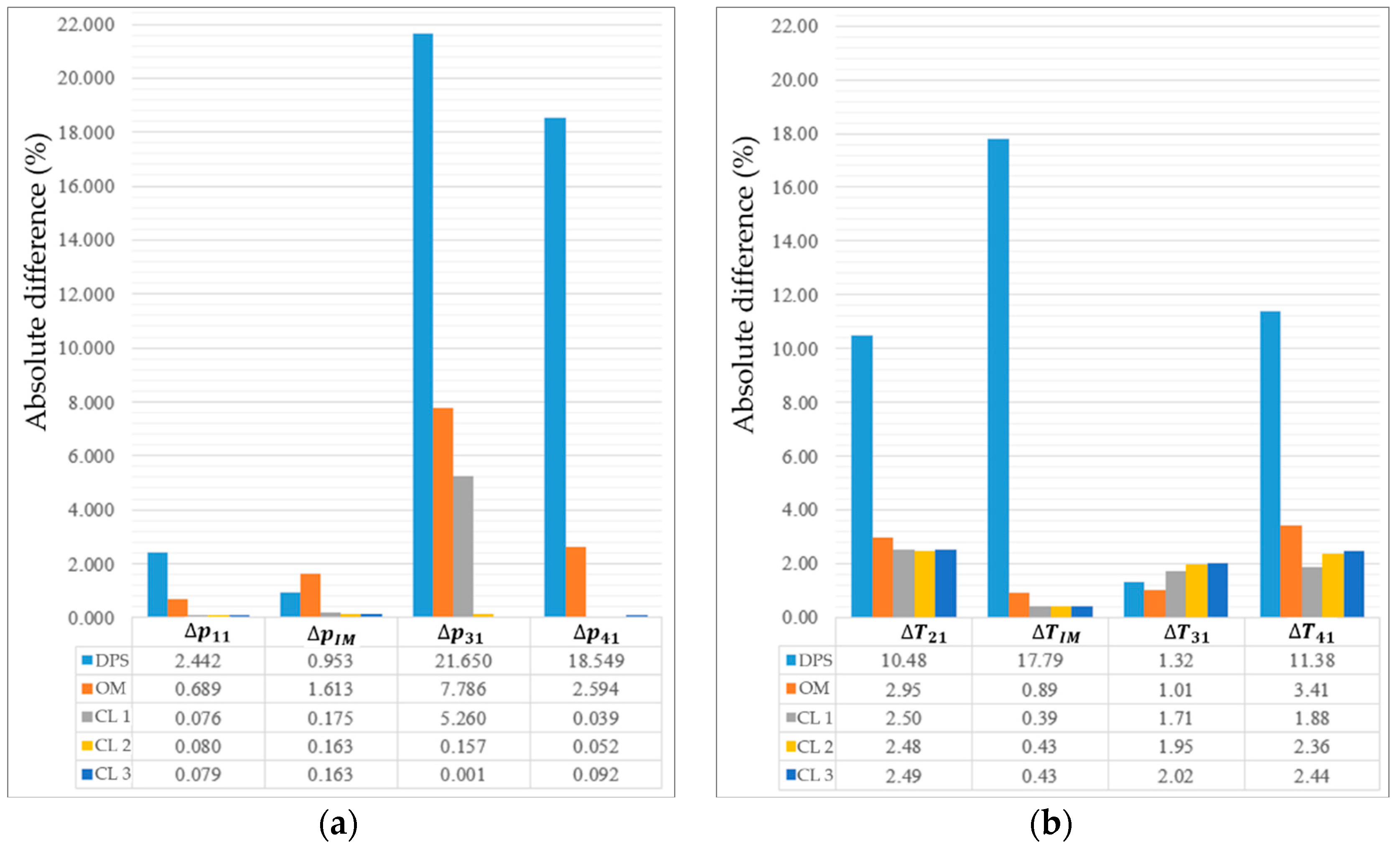
Figure 9 show that there exists a need for performing a calibration of the CBPs of the applied ICESM after model creation is finished as default parameter values (CBPs), although featuring plausible values, do not achieve very good agreement with measurement results.
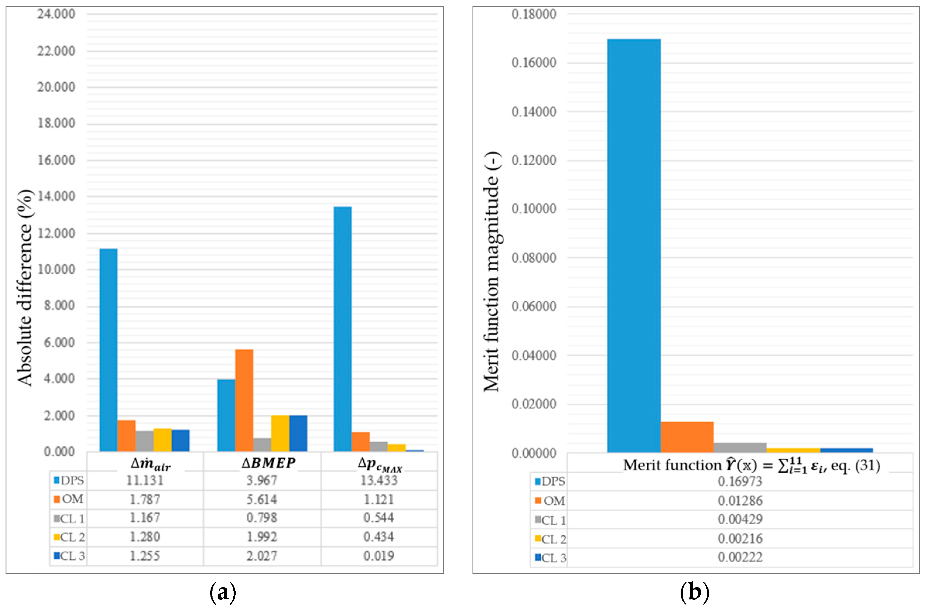
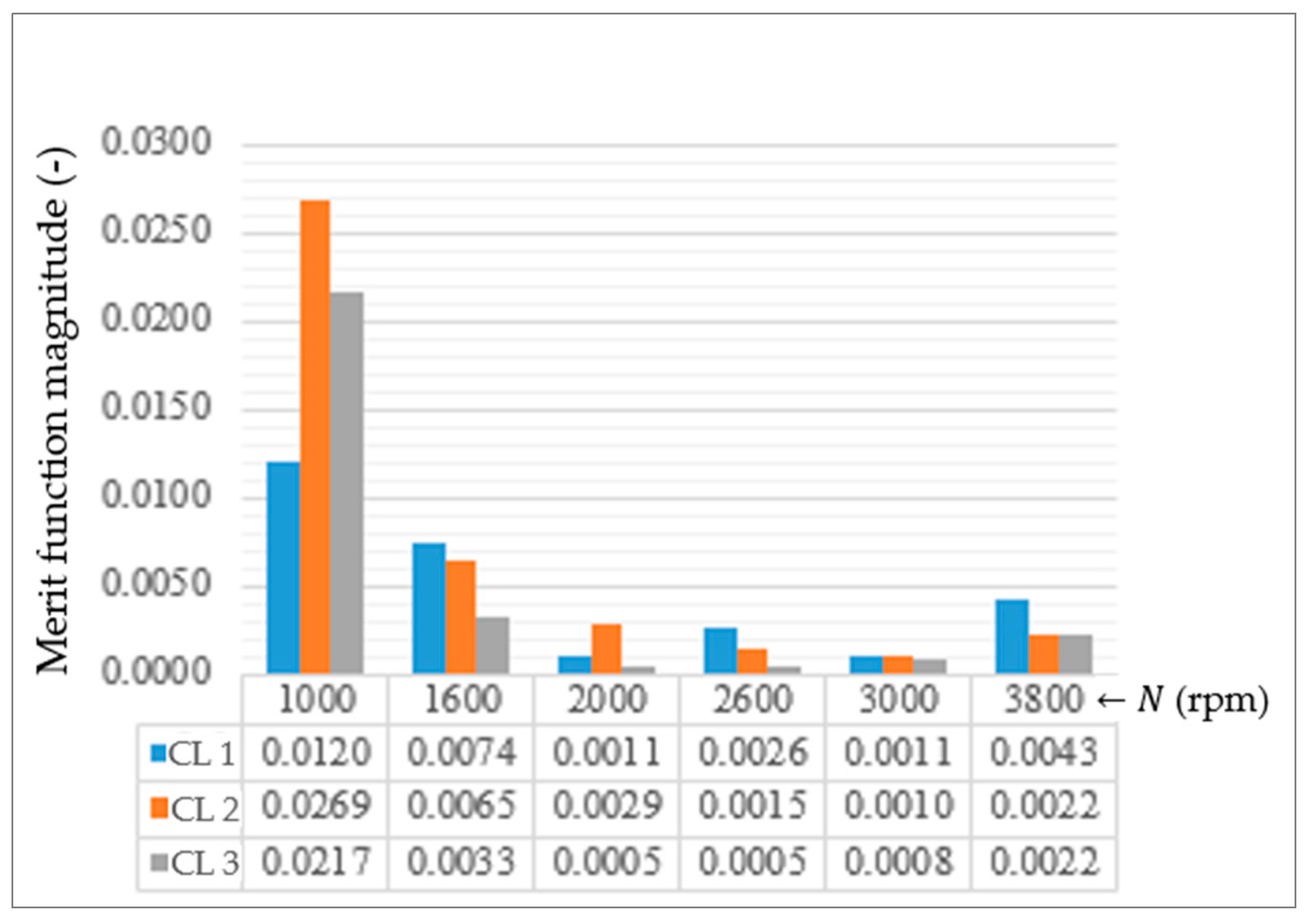
The merit function presented in
Figure 9b, whose magnitude in the ideal case should be 0, indicates the highest magnitude (several times higher than the merit function obtained by the OM and the HCM approach) when the default parameter values of the CBPs are employed in the ICESM.
The merit function of the one-step optimization method (OM) to optimize all CBPs at once shows a better result than the DPS method but the values of the merit function are still far from 0, thus indicating a clear potential for further improvements. An additional drawback of the OM is highlighted by the large values of the
and
(Equation (33)) presented in
Figure 8a and
Figure 9a. Especially the larger deviation of the
is crucial because it is one of the key simulation results of the ICEs simulations. In general,
should be below approximately 3%, being a much smaller value than the one achieved after calibration with the OM. Furthermore, OM converges to multiple solutions with five sets of CBPs, all with a similar
, and additionally consumes more time for the ICESM calibration than HCM as shown in
Figure 10.
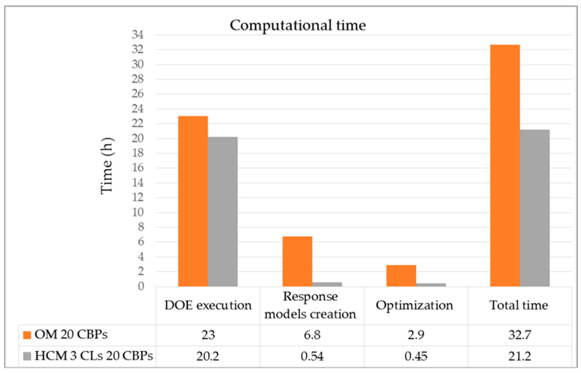
Details of the HCM (
Figure 4) are discussed in
Section 5.2; therefore, only basic data required for the comparison of the computational time between the one-step optimization method and the HCM are provided here. The HCM comprised 2928 simulations (20 CBPs) whereas the one-step optimization method comprised 3260 simulations (20 CBPs). Simulations were carried out on a Windows 7 PC with i7-4800MQ CPU @ 2.7 GHz using four CPUs in parallel for DoE executions whereas a single CPU was used for the remaining tasks presented in
Figure 10.
The HCM features the best results with an approximately six-times-smaller magnitude of the merit function than OM and a 78-times-smaller magnitude than DPS. Additionally the HCM features a higher level of robustness and better controlled convergence to the minimum of the merit function due the conceptual design introduced in
Section 4. Furthermore, a discernible advantage of the HCM is the 35% reduction in consumed computational time for the applied ICESM calibration as presented in
Figure 10. HCM is generally faster than OM in all four compared calibration tasks shown in
Figure 10. A discernible advantage of HCM is observed in the reduced computational time of the response model creation and the CBP search with the RSM-based optimization due to the smaller number of CBPs in one calibration loop (eight, eight, and two (
Section 5.2) vs. 20).
It can thus be concluded that the HCM fulfilled all the requirements raised in the Introduction and that it also performs better than the OM. Therefore, the HCM represents a unique and powerful workflow for the modern ICESM calibration with a large number of calibration parameters.
5.2. Results Obtained with Hybrid Calibration Method
To provide a deeper insight into the calibration workflow in STEP 1 and in STEP 2 of the HCM, this section presents and discusses results obtained with the physics-based approaches and optimization methods presented in
Section 4.4 and
Section 4.5.
The calibration procedure with the applied entire ICESM was performed at four full-load operating points and six part-load steady-state operating points. Full-load operating points covered engine speeds of 1000, 2000, 3000 and 3800 rpm whereas part-load operating points covered engine speeds of 775, 1000, 1600, 1800, 2200 and 2400 rpm. However, validation of the simulation results at full load was performed at six operating points with the objective to verify the capability of the HCM in the operating points that were not subjected to the calibration procedure.
The calibration procedure of the entire ICESM consisted of three calibration loops which comprised full-load and part-load operating points. Calibration loops (
Section 4.5.4) at full-load operating points comprised the following number of CBPs: eight (calibration loop 1), eight (calibration loop 2), two (calibration loop 3); calibration loop 3 at part-load operating points comprised three CBPs (
Table 1). During the calibration process of the sub-systems (
Section 4.4 and
Section 4.5.1), the following number of CBPs was involved: one (SS 1), two (SS 2), one (SS 3), two (SS 4), two (SS 5), one (SS 6). CBPs presented in table form in the following sub-sections apply the same nomenclature of the CBP superscripts as
Table 1.
The DoE plan for the RSM-based optimizations comprised, at full-load operating points, in calibration loop 1 and calibration loop 2 covered 1304 simulations per one loop (326 per one engine speed) and 320 simulations in calibration loop 3. Additionally, calibration loop 2 covered 720 simulations at part-load operating points whereas calibration loop 3 covered 320 simulations.
5.2.1. Results of Physics-Based Calibration of Sub-Systems SS 1–4
This section comprises results of the CBPs obtained in STEP 1 with the employed physics-based approaches discussed in
Section 4.4 and
Section 4.4.1. CBPs of the air cleaner, intercooler, catalyst and EGR cooler (
Section 4.4.1) determined with the employed inverted equations presented in
Section 3.1.8 and
Section 3.1.9. (Equations (13), (19) and (20)) are presented (
Table 1).
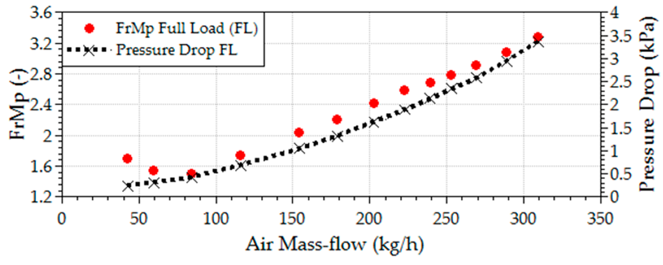
As indicated in the Introduction, tuning parameters are employed due to the inability of the 0D and 1D models to fully capture the 3D fluid flow and heat transfer phenomena, which are additionally coupled with mass transfer phenomena and chemical kinetics mechanisms during fuel injection, evaporation and the combustion phase. Moreover, very detailed geometrical parameters are also very often not known exactly when setting up a system-level simulation.
Figure 11 thus shows the importance of introducing tuning parameters to reproduce experimental results for the case of an air cleaner.
Figure 11 indicates that the measured pressure drop exhibits an approximately quadratic trend with the increasing air mass-flow. Although Equation (20) includes a quadratic velocity term and pipe friction coefficient determined through empirical correlation (Equations (21) and (22)), it can be seen in
Figure 11 that after calibration, values of the
FrMp differ by more than a factor of two due to the reasons exposed at the beginning of this paragraph. This illustrative example clearly exposes the need to include the tuning parameters to allow for reproducing experimentally measured trends.
CBPs of the air cleaner, intercooler, catalyst and EGR cooler (
Section 4.4.1) that were determined through the physics-based calibration are listed in
Table 4 for full-load operating points and in
Table 5 for part-load operating points. Similar to an air cleaner, the
FrMp of the intercooler and EGR cooler indicates a similar magnitude range. Furthermore, due to unknown detailed geometrical parameters of the EGR cooler, the
HTMp of the EGR cooler features values up to 14 (
Table 5).
5.2.2. Results of the Optimization-Based Calibration of the Turbocharger Sub-System (SS 5)
Two CBPs of the turbocharger sub-system (
Section 4.5.1) determined in STEP 1 with the direct search optimization method (
Section 4.5) are outlined in
Table 6.
The turbine HTMp attains values up to 21. This is reasoned by the lack of detailed geometrical data and mainly due to the application of a simple heat transfer correlation.
5.2.3. Results of the Entire ICESM Calibration
This section comprises, in table form, results of all the CBPs determined according to the HCM workflow (
Figure 4) in STEP 2 (
Section 4.5.4). CBPs are determined in calibration loops 1–3 (
Table 1).
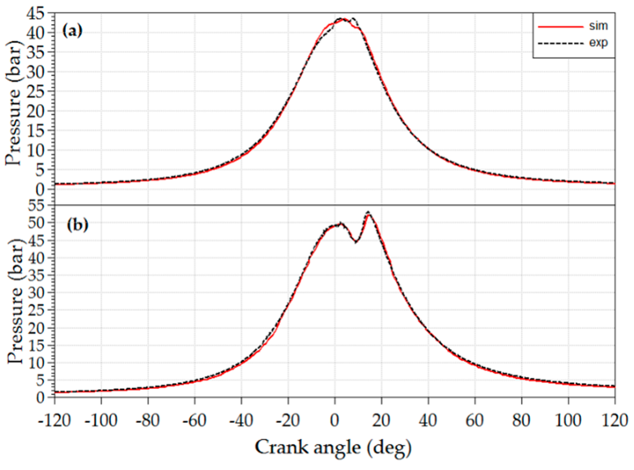
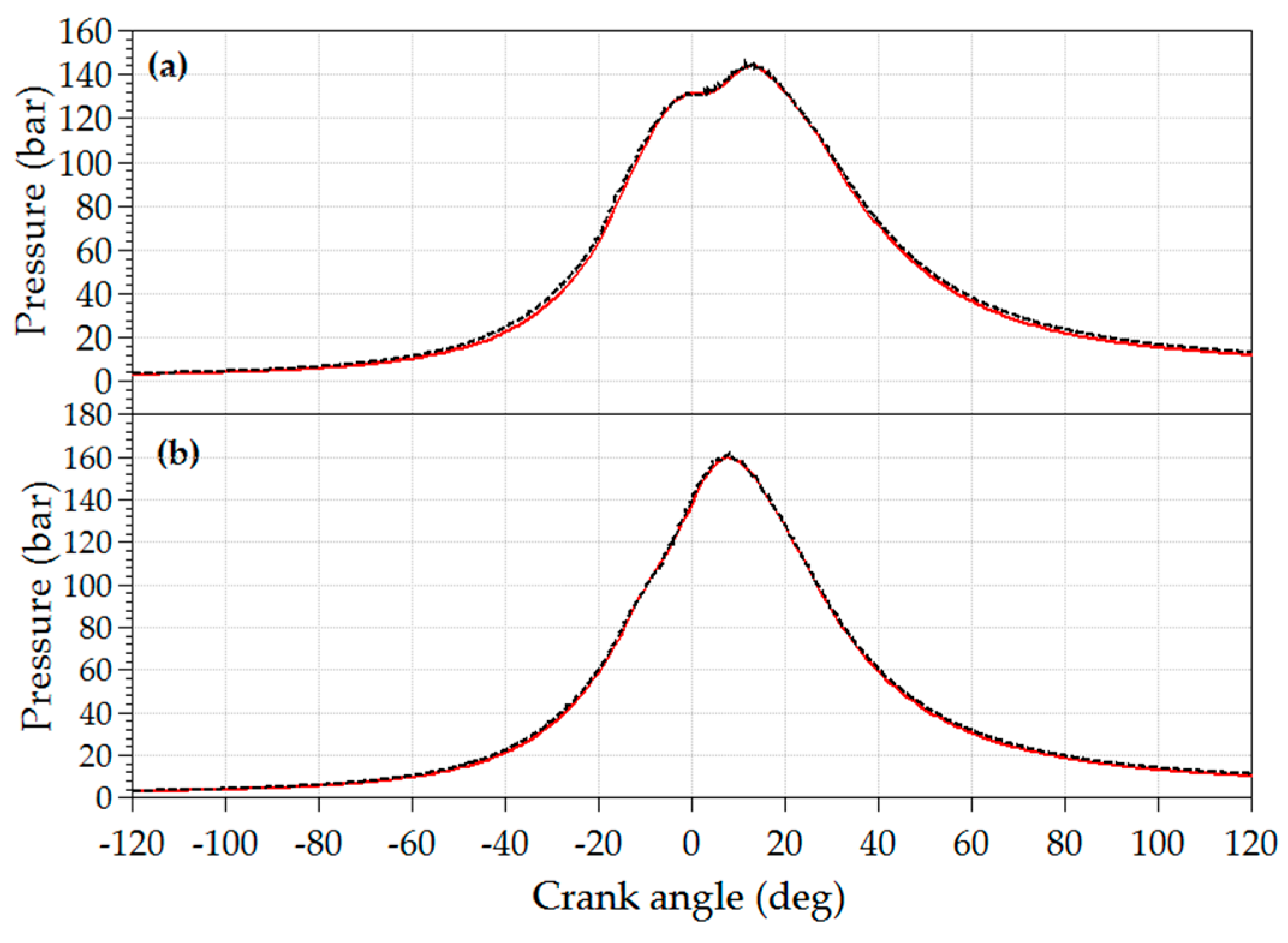
Additionally, agreement between the results of simulations and measurements (e.g.,
Table 2) obtained with the CBPs employed from STEP 1 and STEP 2 in the applied ICESM (
Figure 1) are presented, including cylinder pressure traces and the trends of the merit function. Results of the CBPs obtained at full-load operating points with respect to calibration loops 1–3 are listed in
Table 7,
Table 8 and
Table 9, and at part-load operating points in
Table 10, respectively.
Comparison of the results for the:
CBP 16 indicates that the CBP changes the values in each calibration loop as shown in
Table 7,
Table 8 and
Table 9. Calibration in multi-loops improves the final agreement between the results of the simulation and measurements as shown in
Figure B1c (
Appendix B).
CBP 8 listed in
Table 7 and
Table 9 also indicates different values in calibration loop 1 and calibration loop 3 and enables a stepwise improvement of the simulation results as presented in
Figure B1j.
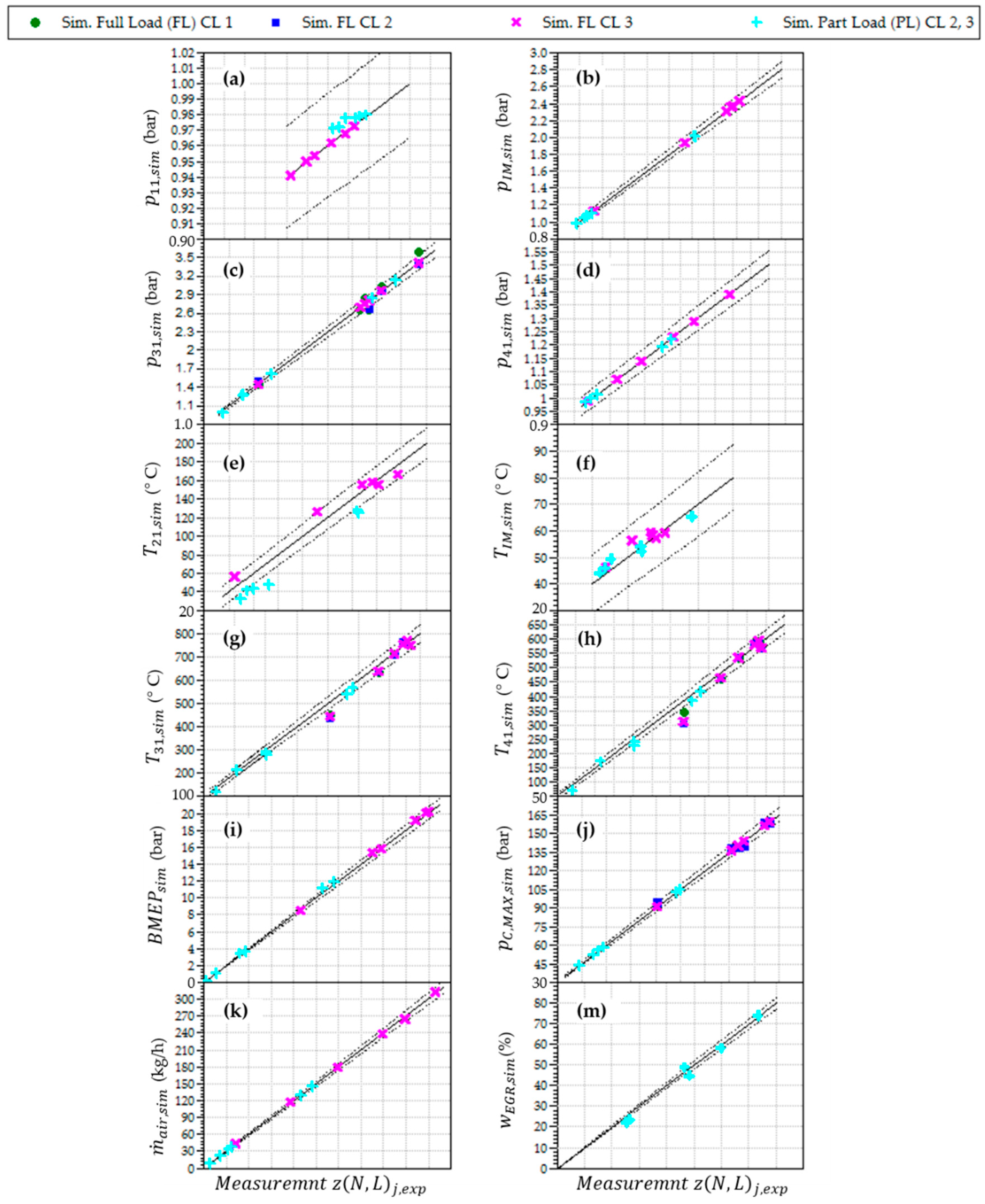
In
Figure B1a–m, comparisons are presented between the results of the simulations and measurements at steady-state operation for six full-load and six part-load operating points. Results are compared in the form of parity plots including the deviation interval ±3.5%, marked with dotted lines. Measurement data are presented with x-axes whereas simulation results of the same quantity are presented with y-axes.
Figure B1m shows only the result of the part-load operating points (EGR is closed at full load). In all the remaining figures in
Figure B1 the simulation results of calibration loop 3 are presented. In
Figure B1c,g,h,j also the results of calibration loop 1 and calibration loop 2 are presented with the aim to identify their influence on the achieved simulation results.
The following conclusions can be summarized from the result comparisons
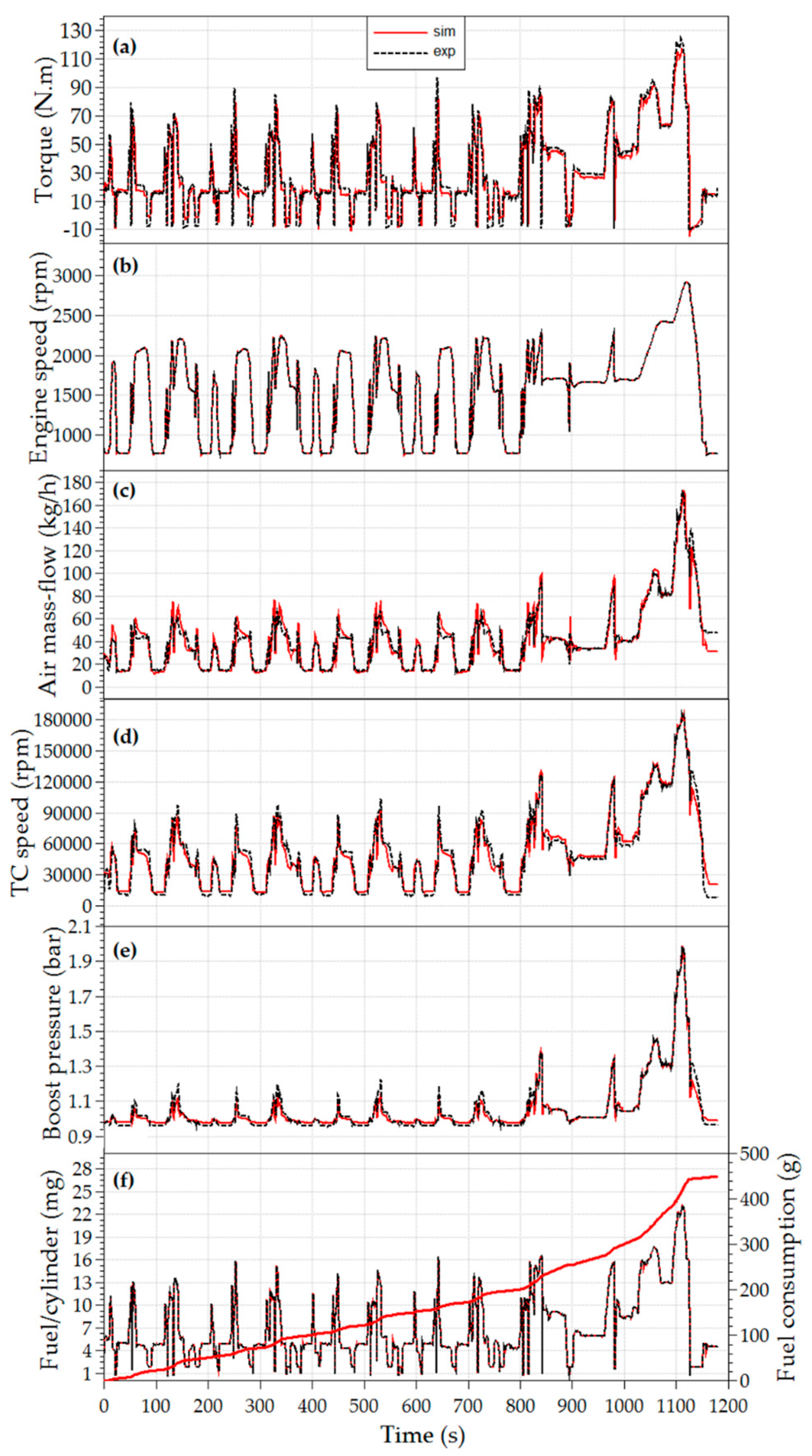
Figure C1 (
Appendix C) shows, compared to the steady-state results, good agreement between the results of the simulations and measurements during hot transient operation of the New European Driving Cycle (NEDC).
6. Conclusions
An innovative Hybrid Calibration Method (HCM) for high fidelity calibration of system-level ICE simulation models featuring a large number of tuning parameters is proposed in this paper. The innovativeness of the method arises for the novel interaction between optimization methods and physically-based methods for calibrating parameters in selected ICE sub-systems. HCM thus relies on consistent division of the simulation model of the ICE on sub-systems based on the available measurement data. The calibration process of the innovative HCM is performed in two steps. The first step comprises the determination of the calibration parameters of sub-systems applying physics-based approaches and the determination of parameters using the direct search procedure. The second step comprises calibration of the reduced number of parameters in several loops at the level of the entire ICESM. RSM-based optimization methods are employed in the second step. In the case of large numbers of remaining parameters for the second step, a multi-loop approach with systematic classification of calibrating parameters is proposed. This approach allows for omitting or at least significantly reducing issues imposed by the weak linear independence of particular sets of CBPs and therefore enables more robust and accurate calibration. Furthermore, in comparison with the one-step optimization method, HCM features shorter calibration times. It can thus be concluded that HCM presents a promising approach for calibrating modern system-level ICE simulation models as it allows for the calibration of a large number of tuning parameters in a robust, repeatable and time-efficient manner.
The HCM presented in this work represents a methodological background of the calibration procedure of ICESM, which is intended to be implemented in an ICE modeling tool to support automatic execution of the entire HCM workflow, as indicated in the paper. The framework features a high level of generality to cover various engine topologies and is, to a large extent, flexible, depending on available measurement data, which, however, certainly influences the fidelity of the method as is also the case for all other calibration methods. Applicability of the HCM is general and it can be applied also to non-ICE-related applications; however, this lies outside of the scope of this paper.


