Article

Static Formation Temperature Prediction Based on Bottom Hole Temperature

1
School of Energy Resources, China University of Geosciences, Beijing 100083, China
2
Department of Petroleum and Geosystems Engineering, University of Texas at Austin, Austin, TX 78712, USA
3
Petroleum Engineering College, Yangtze University, Wuhan 430100, China
*
Author to whom correspondence should be addressed.
Energies 2016, 9(8), 646; https://doi.org/10.3390/en9080646
Submission received: 4 June 2016 / Revised: 29 July 2016 / Accepted: 2 August 2016 / Published: 17 August 2016

Abstract

:
Static formation temperature (SFT) is required to determine the thermophysical properties and production parameters in geothermal and oil reservoirs. However, it is not easy to determine SFT by both experimental and physical methods. In this paper, a mathematical approach to predicting SFT, based on a new model describing the relationship between bottom hole temperature (BHT) and shut-in time, has been proposed. The unknown coefficients of the model were derived from the least squares fit by the particle swarm optimization (PSO) algorithm. Additionally, the ability to predict SFT using a few BHT data points (such as the first three, four, or five points of a data set) was evaluated. The accuracy of the proposed method to predict SFT was confirmed by a deviation percentage less than ±4% and a high regression coefficient R2 (>0.98). The proposed method could be used as a practical tool to predict SFT in both geothermal and oil wells.

Graphical Abstract

1. Introduction

Deep drilling is necessary for the exploitation of deep geothermal reservoirs [1]. In this case, borehole drilling is a complicated process in which a constant thermal anomaly (in addition to the circulating drilling mud) affects the static formation temperature (SFT) around the borehole [2]. Determining SFT at any depth demands a lot of time to measure the bottom-hole temperature (BHT) and shut-in time [3]. Measuring BHT can be costly due to the usage of sophisticated logging equipment and the necessity to temporarily stop the wellbore drilling [4].
Optimal estimation of SFT is required for several applications, including the determination of geothermal heat flow, analysis of well logs, estimation of geothermal potential, evaluation of in situ thermophysical formation properties [5], and the determination of hydrocarbon properties in petroleum systems [6,7,8].
Estimation of SFT is usually achieved by analytical and numerical simulation methods. Most of the analytical methods are based on the constant linear and cylindrical heat source models. Analytical methods most commonly used to estimate SFT include the Horner-plot method (HM), or the line-source method [9]; the Kutasov-Eppelbaum method (KEM), or the generalized Horner method [10]; the Manetti method (MM), or the cylindrical source with a conductive heat flow method [11]; the Hansan and Kabir method (HK), or the cylindrical heat source with a conductive-convective heat flow method [12]; the Bernnand method (BM), or the radial source with a conductive heat flow method [13]; the spherical and redial heat flow method (SRM) proposed by Ascencio et al. [14]; and the Leblanc method (LM), or the cylindrical source with a conductive heat flow method [15].
These methods determine SFT by using BHT and shut-in time data as input, and the linear or nonlinear regression models as solutions [16]. Nevertheless, large errors are likely encountered in the prediction of SFT. In this case such errors may arise from various sources, including unrealistic models proposed to describe the drilling process, heat transfer models based on simple assumptions, measurement errors in the BHT data, and total uncertainties in SFT estimation [17].
Numerical simulation is another method to estimate SFT, which can also be applied to determine geothermal gradients and describe the thermal history [18]. For example, Garcia et al. [19] developed the numerical simulator TEMLOPI for estimating the transient temperature distribution in a wellbore and the surrounding rock formation. Application to well Az-29 from the Los Azufres Mexican geothermal field shows satisfactory results. This simulator could be used by drilling engineers to determine the optimal design of cement slurries and their setting times during well construction.
However, both analytical and numerical simulation methods have some limitations, such as the excessive amount of some other data that is needed in addition to BHT and shut-in time, (e.g., thermophysical and transport properties of the wellbore, drilling and cementing materials, and formation and rock materials, whose data is rarely available and, therefore, limits the usage of these methods) and the accurate circulation time that is usually unknown or difficult to determine under drilling conditions.
Against this background, a reliable and practical tool to estimate SFT is still required in geothermal and petroleum industries. In this paper, a mathematical function has been proposed to correlate BHT and shut-in time. The coefficients of the function were obtained from the particle swarm optimization (PSO) algorithm based on the least squares fit target.
PSO is a stochastic, population-based optimization method that was introduced by Kennedy and Eberhart [20]. It belongs to the family of swarm intelligence computational techniques and is inspired by social interaction in human beings and animals (especially bird flocks and fish schools). PSO optimizes a problem by having a population of candidate solutions, dubbed particles here, and moving these particles around in the search-space according to simple mathematical formulae over the particle’s position and velocity. Each particle’s movement is influenced by its local best known position, but is also guided toward the best known positions in the search-space, which are updated as better positions are found by other particles. The PSO algorithm has been used in many numerical solution problems and shows its wide applicability [21,22,23].
PSO has some advantages in solving optimization problems, for example, it requires few parameters to be tuned by users, it is highly accurate, it is less affected by initial solutions compared with other algorithms, it has fast convergence, and it is easy to code due to the simple underlying concepts and demands no requirement for preconditions, such as continuity or differentiability of the objective functions [24].

2. Methodology

A function correlating BHT and shut-in time was derived to fit the BHT data and the estimated SFT. The coefficients of this function can be obtained from least squares fit method using the particle swarm optimization (PSO) algorithm. Additionally, other methods were also introduced for comparison purposes with the new method. Statistical tests were applied to evaluate the validity of the predicting methods.

2.1. Method Development

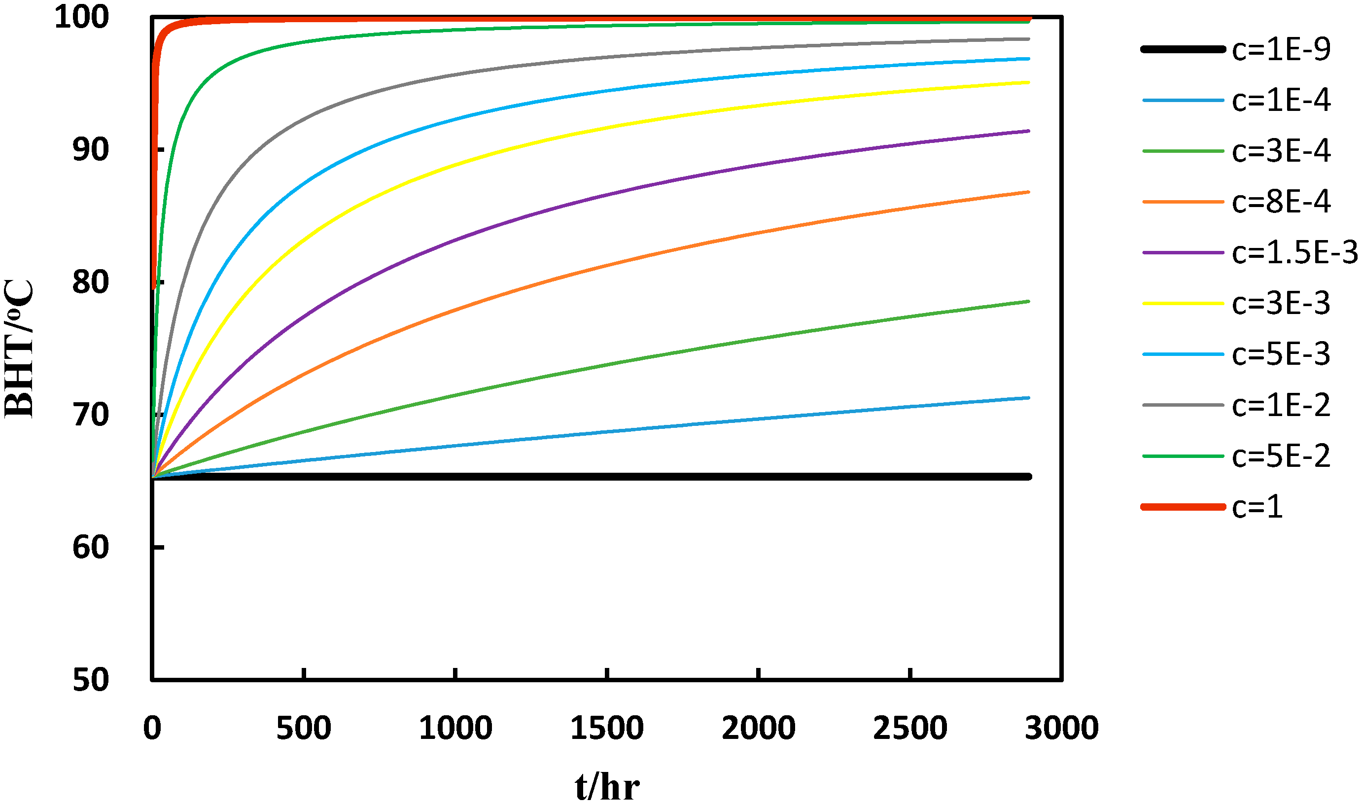
2.1.1. Function Derivation

The Horner method for determining the static formation temperature is widely used in the oil and gas industry [9]. This analytical method is based on the assumption that thermal effect of drilling is a constant linear heat source. The approximate solution is given by:
BHT ( t ) = T H M ( b H M ) ·  log { ( t C + t ) / t }
where T H M is the static formation temperature,  log { ( t C + t ) / t } is the dimensionless Horner time (DHT), and t C and t are the circulation time before shut-in and the time elapsed since the circulation stopped, respectively. One of the problems in Equation (1) is that of being inconsistent with the boundary conditions. BHT approaches the static formation temperature, T H M when t approaches to infinity. However, BHT cannot be obtained when t approaches or is equal to zero. This problem may also decrease the fitting quality of the model. We propose the following mathematical model in order to solve this problem in Equation (1). The modified model is expressed as:
BHT ( t ) = a b   ·  log { 1 ( 1 + c   ·   t ) + 1 } .
where a, b, and c are constants, a is actually equal to T H M , which can be estimated using Equation (2) when shut-in time tends to infinity:
SFT ^ = lim t BHT = a
Equation (2) meets all of the boundary (time) conditions:
As t approaches infinity, maximum BHT is obtained:
BHT m a x = T H M = a
When t approaches to zero, the minimum BHT is obtained:
BHT m i n = a b   ·  ln 2
One can observe that the problem in Equation (1) has now been solved by Equation (2). When the maximum and minimum values of BHT have been determined, the shape of the BHT-time curve will only depend on the value of c. The curve of the BHT-time function is illustrated in Figure 1. The equation can characterize the BHT-time function in a large scope, as shown in Figure 1.

2.1.2. Solutions to the Three Parameters in the New Function

In order to obtain the best fit of the equation, the least squares fit target is applied. The difference between the proposed function and the measured value of temperature is denoted by Q, which is obtained using the following equation:
Q = i = 1 n ( BHT i BHT c i ) 2
where BHT i and BHT ci are measured and calculated BHT using Equation (2).
The least squares fit method requires minimization of Q. Here we used the particle swarm optimization (PSO) algorithm to obtain the best fitting coefficients of a, b, and c that yields the minimum value of X.
The position and velocity of the ith particle are respectively denoted by X i and V i , which are the best position and velocity attained by each particle and therefore referred to as its personal best. For the ith particle, the position vector of its personal best is denoted by P i and its objective value is denoted by P b e s t . The best position attained by the swarm is referred to as either the swarm best, global best, or leader. It is denoted by P g and its objective is denoted by g b e s t . At each iteration t, the positions and velocities of all particles are updated by Equations (7) and (8) which are also called the update equation [24]:
V i ( t + 1 ) = ω V i ( t ) + C 1 r 1 ( P i X i ) + C 2 r 2 ( P g X i )   ( i = 1 , 2 , ,   N P )
X i ( t + 1 ) = X i ( t ) + V i ( t + 1 )   ( i = 1 , 2 , ,   N P )
where ω is inertia weight; C 1 is the cognitive acceleration coefficients, which prompts the attraction of the particle towards its own personal best; C 2 is the social acceleration coefficients, which prompts the attraction of the particle towards the swarm best; and r 1 and r 2 are two random numbers in [0,1].
A schematic of the solving process of the proposed method is depicted in Figure 2.

2.2. Existing Methods

2.2.1. Selection of the Analytical Methods

A few previous analytical methods have been discussed in this paper for comparison with the newly-proposed method in this paper. The three most commonly used analytical methods were introduced in Table 1. The equations, analytical models and sources of these methods are listed in Figure 1. Basically, two regression models were applied to obtain the coefficients in each analytical method.

2.2.2. Selection of the Regression Models

Two regression methods were used as regression models to obtain the coefficients in the three analytical methods: the ordinary linear regression (OLR) model and quadratic regression (QR) model.
The general equation of the OLD model is: y = a + bx , where a and b are the intercept and the slope of the fitted straight line [16], while that for the QR model is given by: y   = a + bx + c x 2 , where a, b, and c represent the polynomial coefficients [16].

2.3. Statistical Evaluation

2.3.1. Deviation Percentages (DEV%)

In order to test the estimation accuracy of the estimated SFT, the deviation percentages (DEV%) between the estimated and reference SFT values were used:
DEV % = [ ( S F T ^ S F T ) S F T ] × 100
where S F T ^ is the value of SFT estimate, and SFT is the true SFT value reported in the literature.
It should be noted that this evaluation test was not applied from datasets without reference SFT (Data 7 and Data 8). The closer the DEV% to zero, the better the estimation of SFT.

2.3.2. Regression Coefficient (R2)

The regression coefficient (R2) is applied for testing the fitting ability of each method. The value can be obtained from:
R 2 = 1 ( y i y ^ i ) 2 ( y i y ¯ ) 2 .
where y i is the measured value of BHT, y ^ i is the estimated BHT, and y ¯ is the mean of the measured BHT values. The fitting is more satisfactory if the value of R2 is closer to 1.

2.3.3. Residual Sum of Squares (RSS)

The fitting result of each method can also be evaluated through estimation of the normalized residual sum of squares (RSS), which is calculated by the following equation:
RSS = i = 1 n ( y i y ^ i ) 2 n .
where y i and y ^ i are same as in Equation (10), n is the total numbers of elements in a BHT dataset. The smaller the value of RSS in a dataset, the better the fitting result. The goodness of fit can be evaluated by DEV% and R2. However, the comparison between different methods should be based on the whole accuracy and fitting ability of each method. To evaluate each method comprehensively, the following synthetic statistical parameters were also used.

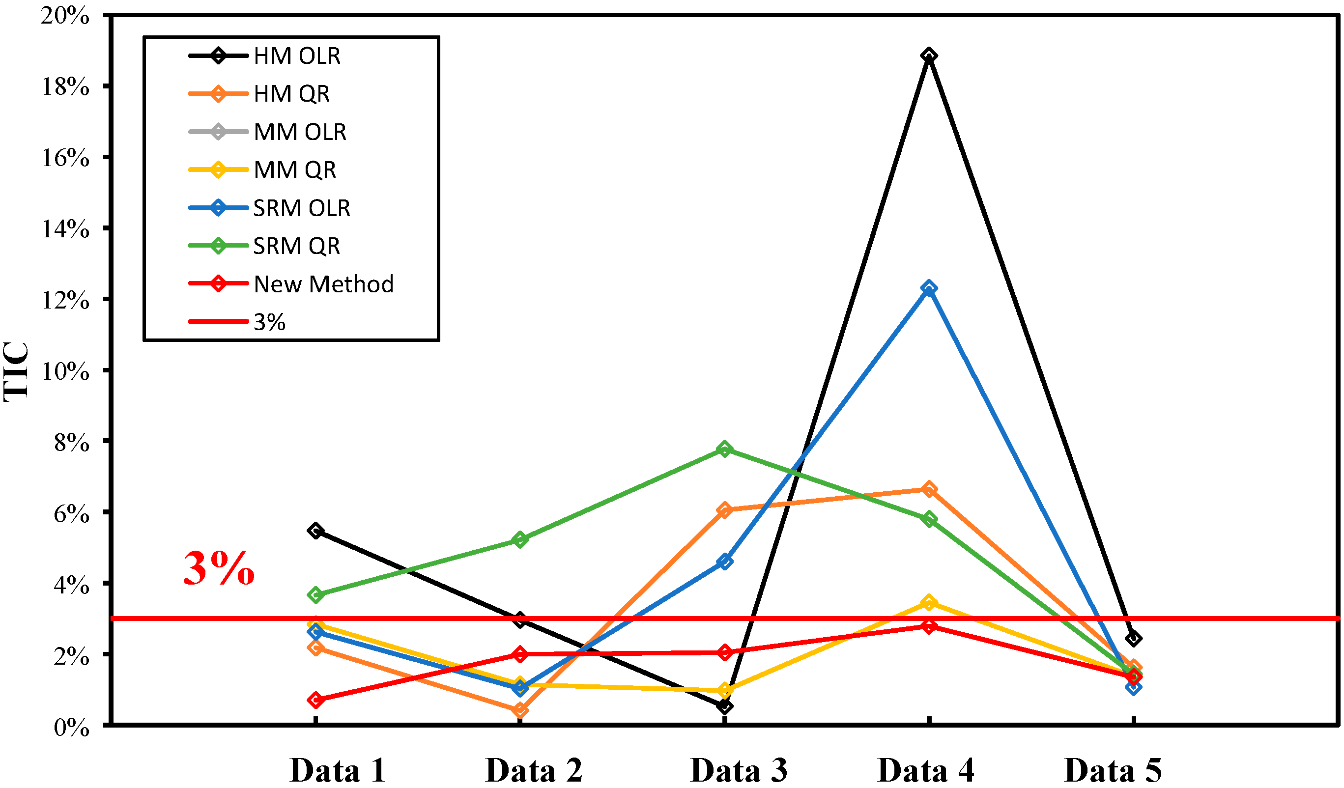
2.3.4. Theil Inequality Coefficient (TIC)

TIC is applied to test the estimation accuracy comprehensively when only very few BHT data are available. For each dataset and each method used, the TIC value can be obtained from:
TIC = i = 3 5 ( S F T ^ i S F T ) 2 i = 3 5 S F T ^ i 2 + S F T
where S F T ^ i is the SFT estimate using the first i of the dataset.
The value of TIC is in [0,1], and could be used to compare between different datasets. For each method, the closer the TIC to zero, the more accurate the method is.

2.4. Data Sources

Eight thermal recovery datasets were collected from the published literature (see Table 2) for the accuracy and application tests. They include:
(1)
Four synthetic datasets selected from the literature; and
(2)
Four datasets logged in some boreholes from long logging work in geothermal and petroleum fields.
These datasets are summarized in Table 2 [25,26,27,28,29,30].
It should be pointed out that the datasets 1–6 all have reference SFT values, which can be very useful to evaluate the application of the proposed method and conduct comparisons between different methods.

3. Validation and Discussion

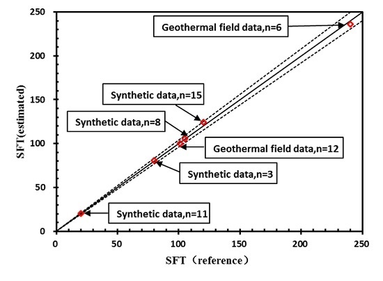
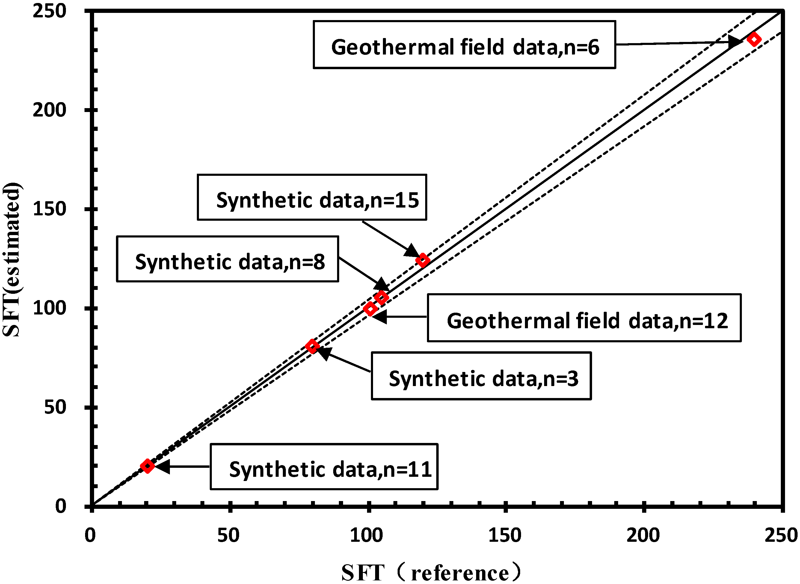
3.1. Accuracy of the Static Formation Temperature (SFT)

For each dataset, coefficients a, b, and c were solved by the PSO algorithm based on the least squares fit target. After applying Equation (2), the BHT data were recalculated at each shut-in time of the borehole and entitled calculated BHT. The DEV% between SFT estimate and reference SFT were obtained by Equation (9), as described in the “Methodology” section. A comparison between data from the literature and data estimated by our proposed method is depicted in Figure 3, in which yellow circles represent measured BHT values (in this case reference BHT), black dots represent calculated BHT, red full lines represent reference SFT, and the black dashed lines represent values of SFT estimate.
Using the synthetic set of Data 1, the SFT value estimated by the proposed method was 80.99 °C, which is in agreement with the true SFT, 80 °C. The error in this case is 1.24%. The SFT estimated in Data 2 is about 4 °C higher than the true value (120 °C), with an acceptable percentage of 3.52%. For those data sets from well-logging (Data 4 and 5), the deviation percentages fall in the range of −2% to 1%. Data 6 was recorded at three shut-in times, with an SFT value of 105.296 °C estimated accurately by the proposed method, and a deviation percentage of 0.28% with the reference SFT value of 105 °C.
Figure 4 shows the comparison between estimated SFT values using the proposed method and true SFT values for six datasets using the true SFT values ranging from 20.25 to 240 °C, during the last shut-in time from 1.5 h to 600 h. The number of the dataset varies from three to 15. The DEV% of each dataset is in [−2%, 4%], a satisfactory range for a practical predicting tool.

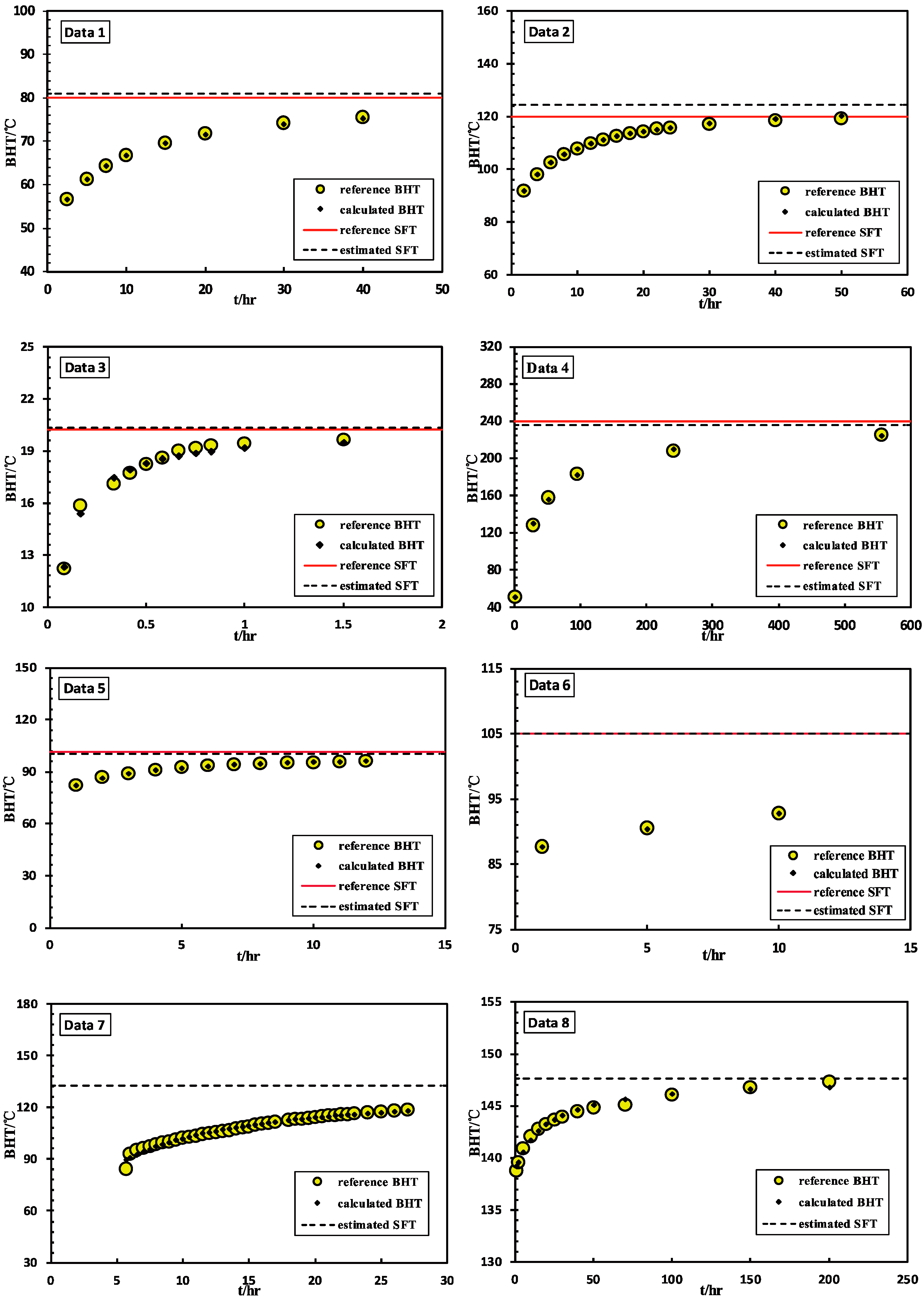
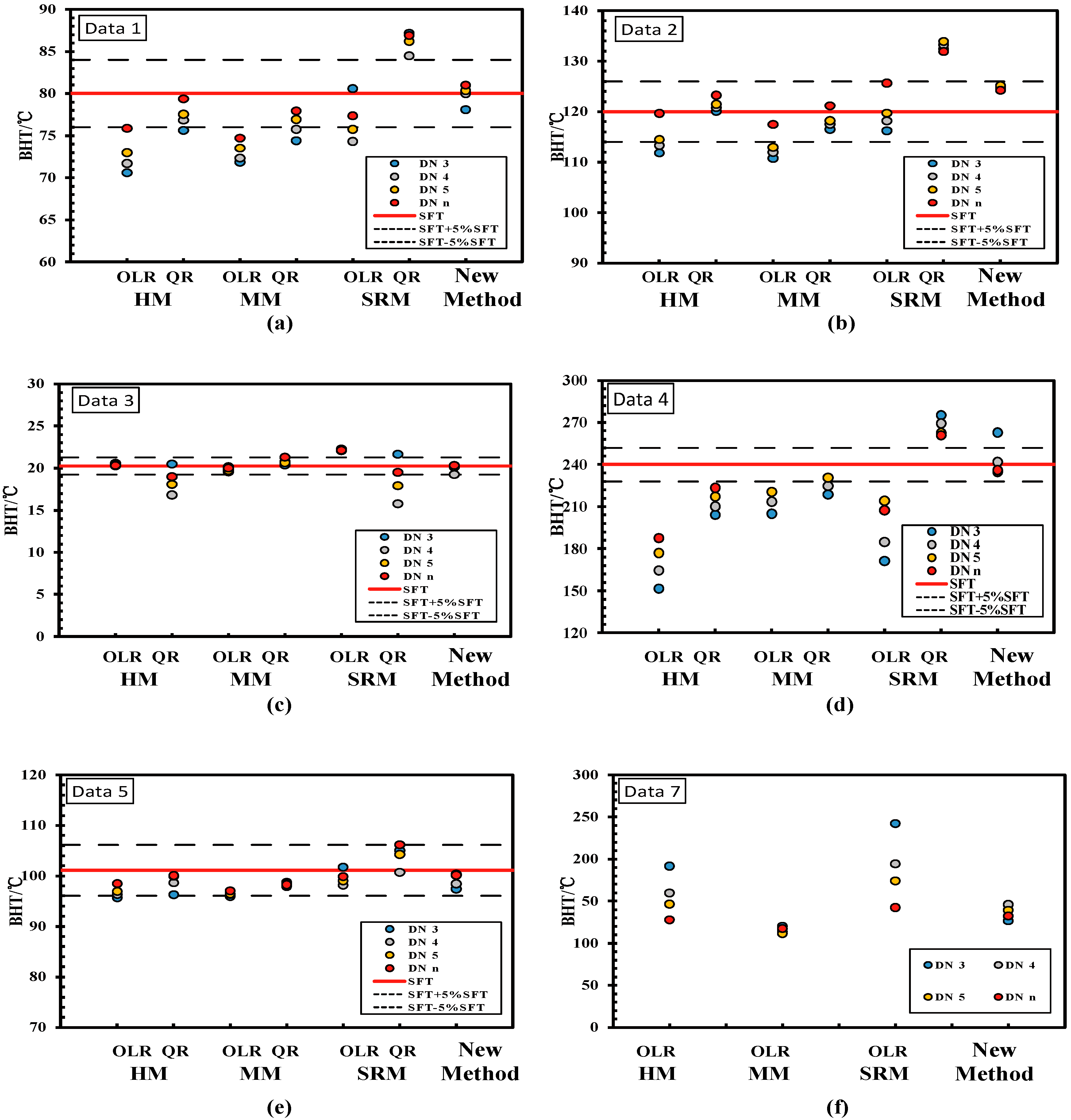
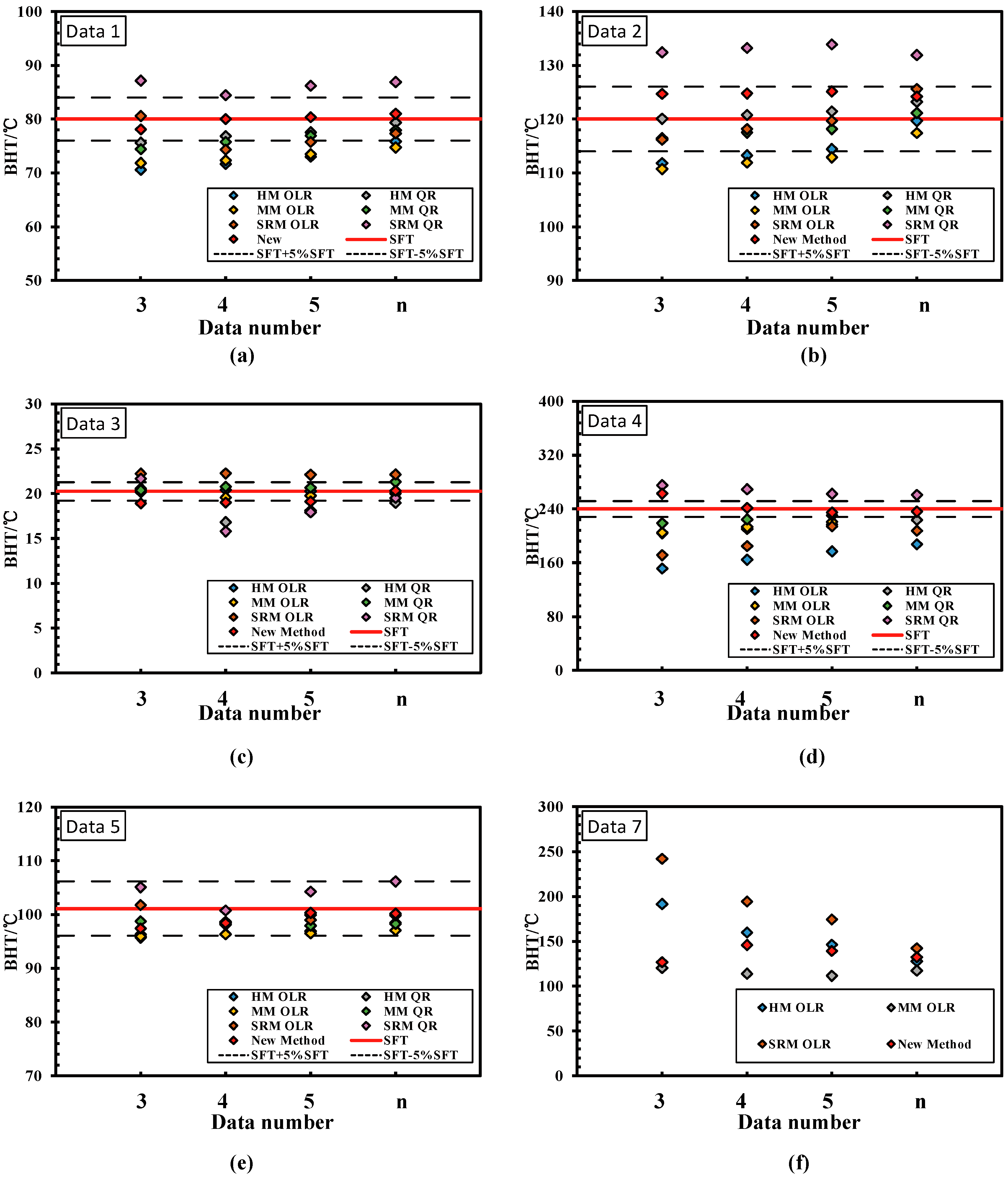
3.2. Fitting Results

The regression coefficients R2 determined by Equation (10) and the normalized RSS by Equation (11) were calculated for all datasets using the proposed method. The calculation results are presented in Table 3, and the BHT values calculated by the proposed method are also shown in Figure 3. For the datasets 1 and 2, the values of R2 are both greater than 99.9%, which indicates that the proposed method can fit the BHT data accurately. As for those BHT datasets obtained from well-logging, the proposed method also showed a good fitting ability because the R2 for each dataset is greater than 98%. Based on the good matching results, the proposed method seems to provide acceptable correlations between BHT and shut-in time.
In addition, comparisons of estimates and reference SFT values using various methods was carried out, the results of which are shown in Table 4. It is obvious that the SFT values predicted by the proposed method are much better than others.

4. Applications in the Case of a Small Number of Data Points

The fitting ability of the proposed method has been tested in the cases of a set having a small number of BHT data points. Three different analytical methods with two different regression models mentioned in Section 2 were applied for comparison, the results were shown in Table 5. The first three, four, or five data points of each dataset were applied to estimate SFT in different analytical methods including the proposed method. The results are discussed in this section.
Figure 5 and Figure 6 present the SFT estimation results using different methods when the first three, four, or five data points or all the n data points in each set (i.e., DN 3, DN4, DN 5, and DN n) are used. The red full line in Figure 5a–f (plotted based on the dataset 1 to 6) represents the true value of SFT for each dataset, whereas the black dashed lines above and below the red line represent the SFT values with the DEV% of 5% and −5% of the true SFT value, respectively. The circles in Figure 5 and the diamonds in Figure 6 represent the results of SFT estimations using different methods. It should be mentioned that the red diamonds in Figure 6 represent the SFT estimates of our proposed method. The results of deviation percentages between each estimate with the reference SFT value are listed in Table 4 for reference. The SFT estimates discussed here were obtained using seven methods when the first three, four, or five points, or all data elements in each set, were applied, in the ranges [SFT −5% SFT to SFT +5% SFT], which is called “the acceptable range”.
By comparing the SFT estimates with the reference SFT values, it can be observed in Figure 5 that the SFT values estimated by the Horner method (HM) when OLR model is applied were typically underestimated in all datasets except for Data 3. Additionally, the aspheric heat-flow method (SRM) with the OLR model was likely to overestimate the SFT, as mentioned in [17]. As for the regression models, results showed that SFT values estimated by using an ordinary linear regression model were less than those by the quadratic regression model in Figure 5. This observation was also reported in other literature [16,17].
For Data 1 and 2 set, the proposed method is the only method in which all the SFT estimates lie in the acceptable range. It can be concluded that both the HM and MM method with the QR model are two good estimating methods, except for the proposed method from Figure 5a,b. However, the SFT estimates obtained using the two methods for only the first three points of Data 1 set were both out of the acceptable range. Estimation results for the Data 3 set using the three methods were all in the acceptable range. The three methods in this case involved HM with the OLR model, MM with the OLR model, and the proposed method. For this dataset use of the SRM methods with the OLR and QR models could not yield good results for the estimated SFT. For Data 4, application of DN 3 in all methods resulted into the SFT being out of the acceptable range. However, it should be noted that the proposed method was the only method in which the estimates laid in the acceptable range (using DN 4, DN 5 and DN n). All but one SFT estimated by the MM method with QR model on the DN n were unacceptable. For Data 5, the predicting results of the proposed method and other four methods all lied in the acceptable range. For Data 7 without the reference SFT value, the predicting ability of each method can still be seen in Figure 5f. The estimates obtained from HM method with OLR model and SRM method with the OLR model were uncertain, with a range of 63.77 °C and 99.74 °C, respectively. However, the proposed method, as well as the MM method with the OLR model, can still be used to estimate SFT reliably. Except for the SRM method with the QR model, using our proposed method, the estimates using other methods were likely to be underestimated when only the first three, four, or five points of the dataset were used, while the estimates by the SRM method with the QR model were more likely to be exaggerated. However, estimates obtained from the proposed method were likely to distribute but close on both sides of the reference SFT value (red full lines in Figure 5), which is also an indication of the advantage of the proposed method.
Based on the results of these statistical tests and the analysis above, the proposed method can be considered to estimate SFT accurately and reliably in the cases with few data.
Both data quantity and method will affect the accuracy of prediction, and some methods under specific conditions may have better results than the newly-proposed method, so the Theil inequality coefficient (TIC), an overall evaluation, was used to assess all of the data. The value of the TIC is in [0,1], and could be used to compare the results of different datasets. For each method, the closer the TIC is to zero, the more accurate that method is. The results of the TIC are depicted in Figure 7. It is to be observed that the new proposed method is the only one in which the TIC values for all datasets are less than 3%, indicating that the newly-proposed method cannot only estimate SFT using a few data points accurately, but also reliably.
Note that the SFT may vary with depth and rock type of the formation because the corresponding thermal stress varies with depth and rock type of the reservoir. This, however, has not been investigated in the current study and a research plan has been embarked to further explore the possible relationship between SFT and depth, as well as rock type.

5. Conclusions

(1)
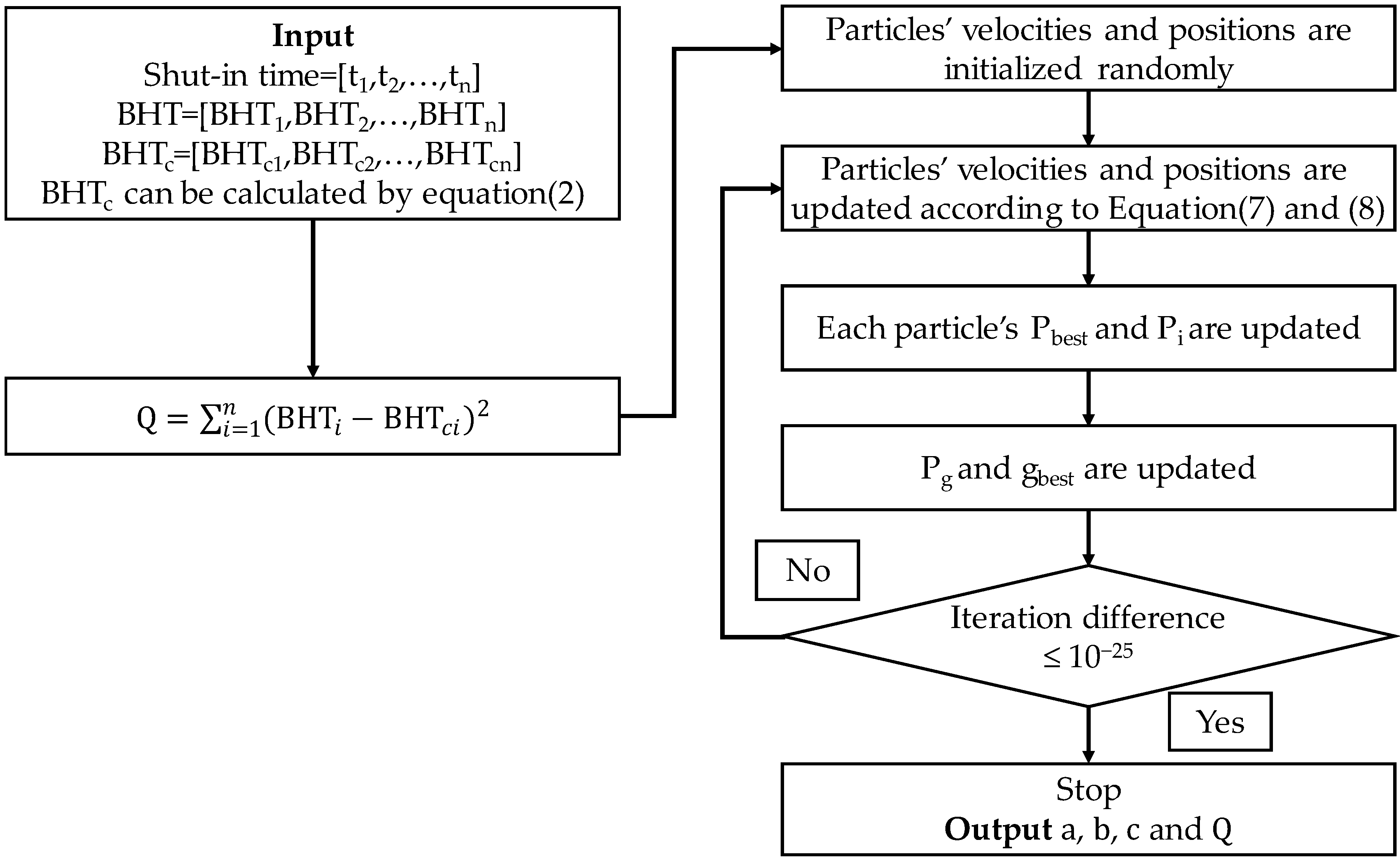
A numerical method was proposed to estimate SFT from the BHT data and shut-in time. The unknown coefficients of the model were derived from the least squares fit by the particle swarm optimization (PSO) algorithm.
(2)
The estimation accuracy and fitting ability of the proposed method was verified using eight BHT datasets, including synthetic, geothermal, and petroleum field data. The deviation percentages are less than ±4% and the regression coefficient R2 are greater than 0.98.
(3)
A comparison among different methods was conducted. The new proposed method could estimate SFT accurately and reliably, even by using a small number of BHT data points (the TIC values for all datasets are less than 3%). This might be used as a practical tool to predict SFT in both geothermal and oil wells.

Acknowledgments

Thanks are due to Youguang Chen, Lin Jia and Dong Ma for assistance with the calculations and to Kewen Li for valuable suggestions.

Author Contributions

This study was done as part of Changwei Liu’s doctoral studies supervised by Kewen Li. Changwei Liu revised the models and conducted the calculations. Kewen Li established the main research ideas and wrote the manuscript. Youguang Chen mainly performed the fitting. Lin Jia and Dong Ma were responsible for the data analysis and editing and of the manuscript.

Conflicts of Interest

The authors declare no conflict of interest.

References

  1. Saito, S.; Sakuma, S.; Uchida, T. Drilling Procedures, Techniques and Test RM Results for a 3.7 km Deep, 500 °C Exploration Well, Kakkonda, Japan. Geothermics 1998, 27, 573–590. [Google Scholar] [CrossRef]
  2. Fomin, S.; Chugunov, V.; Hashida, T. Analytical Modelling of the Formation Temperature Stabilization during the Borehole Shut-in Period. Geophys. J. Int. 2003, 155, 469–478. [Google Scholar] [CrossRef]
  3. Santoyo, E.; Garcia, A.; Espinosa, G.; Hernandez, I.; Santoyo, S. Static_temp: A Useful Computer Code for Calculating Static Formation Temperatures in Geothermal Wells. Comput. Geosci. 2000, 26, 201–217. [Google Scholar] [CrossRef]
  4. Wisian, K.W.; Blackwell, D.D.; Bellani, S.; Henfling, J.A.; Normann, R.A.; Lysne, P.C.; Förster, A.; Schrötter, J. Field comparison of conventional and new technology temperature logging systems. Geothermics 1998, 27, 131–141. [Google Scholar] [CrossRef]
  5. Bassam, A.; Santoyo, E.; Andaverde, J.; Hernández, J.A.; Espinoza-Ojeda, O.M. Estimation of Static Formation Temperatures in Geothermal Wells by Using an Artificial Neural Network Approach. Comput. Geosci. 2010, 36, 1191–1199. [Google Scholar] [CrossRef]
  6. Melton, C.E.; Giardini, A.A. Petroleum Formation and the Thermal History of the Earth’s Surface. J. Pet. Geol. 1984, 7, 303–312. [Google Scholar] [CrossRef]
  7. Armstrong, P.A.; Chapman, D.S.; Funnell, R.H.; Allis, R.G.; Kamp, P.J.J. Thermal Modeling and Hydrocarbon Generation in an Active-margin Basin: Taranaki Basin, New Zealand. Aapg Bull. 1996, 80, 1216–1241. [Google Scholar]
  8. Stephan, K.M. Reservoir Simulation: Mathematical Techniques in Oil Recovery. Geofluids 2008, 8, 344–345. [Google Scholar]
  9. Dowdle, W.L.; Cobb, W.M. Static Formation Temperature from Well Logs—An Empirical Method. J. Pet. Technol. 1975, 27, 1326–1330. [Google Scholar] [CrossRef]
  10. Kutasov, I.M.; Eppelbaum, L.V. Determination of Formation Temperature from Bottom-hole Temperature Logs—A Generalized Horner Method. J. Geophys. Eng. 2005, 2, 90–96. [Google Scholar] [CrossRef]
  11. Manetti, G. Attainment of Temperature Equilibrium in Holes during Drilling. Geothermics 1973, 2, 94–100. [Google Scholar] [CrossRef]
  12. Hasan, A.R.; Kabir, C.S.; Hasan, A.R. Static Reservoir Temperature Determination from Transient Data after Mud Circulation. SPE Drill. Complet. 1994, 9, 17–24. [Google Scholar] [CrossRef]
  13. Brennand, A.W. A New Method for the Analysis of Static Formation Temperature Test. In Proceedings of the 6th New Zealand Geothermal Workshop, Auckland, New Zealand; 1984. Available online: https://www.geothermal-energy.org/pdf/IGAstandard/NZGW/1984/Brennand.pdf (accessed on 4 June 2016). [Google Scholar]
  14. Ascencio, F.; García, A.; Rivera, J.; Arellano, V. Estimation of Undisturbed Formation Temperatures under Spherical-radial Heat Flow Conditions. Geothermics 1994, 23, 317–326. [Google Scholar] [CrossRef]
  15. Lech, P.J.; Pappoe, R.; Nakamura, T.; Russell, S.J. The Temperature Stabilization of a Borehole. Virology 2012, 46, 1301–1303. [Google Scholar]
  16. Espinoza-Ojeda, O.M.; Santoyo, E.; Andaverde, J. A New Look at the Statistical Assessment of Approximate and Rigorous Methods for the Estimation of Stabilized Formation Temperatures in Geothermal and Petroleum Wells. J. Geophys. Eng. 2011, 8, 233–258. [Google Scholar] [CrossRef]
  17. Wongloya, J.A.; Andaverde, J.; Santoyo, E. A new practical method for the determination of static formation temperatures in geothermal and petroleum wells using a numerical method based on rational polynomial functions. J. Geophys. Eng. 2012, 9, 711–728. [Google Scholar] [CrossRef]
  18. Tragesser, A.F.; Crawford, P.; Crawford, H. A method for calculating circulating temperatures. J. Pet. Technol. 1967, 19, 1507–1512. [Google Scholar] [CrossRef]
  19. Garcia, A.; Hernandez, I.; Espinosa, G.; Santoyo, E. Temlopi: A Thermal Simulator for Estimation of Drilling Mud and Formation Temperatures during Drilling of Geothermal Wells. Comput. Geosci. 1988, 24, 465–477. [Google Scholar] [CrossRef]
  20. Kennedy, J.; Eberhart, R. Particle Swarm Optimization. In Proceedings of the IEEE International Conference on Neural Networks, Perth, WA, Australia, 29 November–1 December 1995.
  21. Chen, M.R.; Li, X.; Zhang, X.; Lu, Y.Z. A Novel Particle Swarm Optimizer Hybridized with Extremal Optimization. Appl. Soft Comput. 2010, 10, 367–373. [Google Scholar] [CrossRef]
  22. Ziari, I.; Jalilian, A. Optimal Placement and Sizing of Multiple APLCs Using a Modified Discrete PSO. Int. J. Electr. Power Energy Syst. 2012, 43, 630–639. [Google Scholar] [CrossRef]
  23. Mahor, A.; Rangnekar, S. Short Term Generation Scheduling of Cascaded Hydroelectric System Using Novel Self-adaptive Inertia Weight PSO. Int. J. Electr. Power Energy Syst. 2012, 34, 1–9. [Google Scholar] [CrossRef]
  24. Jordehi, A.R. A Review on Constraint Handling Strategies in Particle Swarm Optimization. Neural Comput. Appl. 2015, 26, 1–11. [Google Scholar] [CrossRef]
  25. Cooper, L.R.; Jones, C. The Determination of Virgin Strata Temperatures from Observations in Deep Survey Boreholes. Geophys. J. Int. 1959, 2, 116–131. [Google Scholar] [CrossRef]
  26. Kutasov, I.M.; Technologies, M.S.; Monica, S. Applied Geothermics for Petroleum Engineers; Elsevier: Amsterdam, The Netherlands, 1999; p. 347. [Google Scholar]
  27. Li, D.X. Non-linear Fitting Method of Finding Equilibrium Temperature from BHT Data. Geothermics 1986, 15, 657–664. [Google Scholar]
  28. Schoeppel, R.J.; Gilarranz, S. Use of Well Log Temperatures to Evaluate Regional Geothermal Gradients. J. Pet. Technol. 1966, 18, 667–73. [Google Scholar] [CrossRef]
  29. Shen, P.Y.; Beck, A.E. Stabilization of Bottom Hole Temperature with Finite Circulation Time and Fluid Flow. Geophys. J. R. Astron. Soc. 1986, 86, 63–90. [Google Scholar] [CrossRef]
  30. Cao, S.; Lerche, I.; Hermanrud, C. Formation Temperature Estimation by Inversion of Borehole Measurements. Geophysics 2012, 53, 979–988. [Google Scholar] [CrossRef]
Figure 1. The relationship between bottom hole temperature (BHT) and shut-in time, when a = 100, b = −50, and c varies from 1 × 10⁻⁹ to 1.
Energies 09 00646 g001
Figure 2. Schematic representation of the solving process of the proposed method.
Energies 09 00646 g002
Figure 3. Comparisons for the bottom-hole temperature (BHT) and Static formation temperature (SFT).
Energies 09 00646 g003
Figure 4. Comparison of the SFT estimates using the proposed method and reference SFT values. (n is the number of data points of each dataset).
Energies 09 00646 g004
Figure 5. SFT estimates for each method using the first three, four, five, or n points of a dataset. (e.g., DN 3 represents use of the first three points of a given dataset, (a) to (f) plotted based on the dataset 1 to 5 and 7).
Energies 09 00646 g005
Figure 6. SFT estimates for each method using the first three, four, or five points, or all (n) data of a set, (a) to (f) plotted based on the dataset 1 to 5 and 7.
Energies 09 00646 g006
Figure 7. Comparison of Theil Inequality Coefficient (TIC) values for each dataset and various estimating methods.
Energies 09 00646 g007
Table 1. A summary of the analytical methods used for comparison with the method developed in this paper.
MethodPhysical ModelEquationSources
Horner (HM)Constant Linear heat source BHT ( t ) = T H M b H M l n ( t + t c t ) Dowdle and Cobb (1975)
Manetti (MM)Conductive cylindrical heat source BHT ( t ) = T M M b M M l n ( t t t c ) Manetti (1973)
Ascencio (SRM)Spherical-radial heat flow BHT ( t ) = T S R M b S R M l n ( 1 t ) Ascencio et al. (1994)
Table 2. Summary of the bottom-hole temperature (BHT) datasets used in this paper.
DataTypentc (h)SourcesData Name in This Paper
SHBESynthetic data85Shen and Beck (1986)Data 1
CLAHSynthetic data155Cao et al. (1988)Data 2
CJONSynthetic data120.2Cooper and Jones (1959)Data 3
KJ-21Geothermal field data62.5Steingrimsson and Gudmundsson (1989)Data 4
SGGeothermal field data123Schoeppel and Gilarranz (1966)Data 5
MOUSynthetic data310Mou (2013)Data 6
DA-XINGeothermal field data405Da-Xin (1986)Data 7
UASMPetroleum field data1410Kutasov (1999)Data 8
Table 3. Results of each dataset using the proposed method.
NO.Coefficients of the Proposed MethodSTFSFTDEV%R2RSS
abc(Reference)(Estimated)
Data 181.00045.9600.17280.00081.0001.2491.0000.025
Data 2124.23263.4590.243120.000124.2323.5270.9990.089
Data 320.32730.86528.29920.25020.3270.3800.9870.073
Data 4236.084280.8370.039240.000236.084−1.6320.9992.243
Data 5100.13221.1110.694101.111100.132−0.9680.9990.026
Data 6105.29626.4810.067105.000105.2960.2821.0000.000
Data 7132.459133.5880.289N/A132.459N/A0.97911.053
Data 8147.60012.8090.071N/A147.600N/A0.9790.085
Table 4. Comparison of estimates and reference Static formation temperature (SFT) values using various methods.
NO.HMMMSRMProposed MethodReference SFT
OLRQROLRQROLRQR
Data 175.87179.37274.71377.93677.36286.91480.99980
Data 2119.66123.26117.45121.15125.63131.91124.231120
Data 320.32818.98120.00321.30222.13219.49920.32720.25
Data 4187.60223.5220.64230.65207.39260.87236.084240
Data 598.449100.0797.04898.25799.858106.16100.133101.111
Data 694.26198.53594.971N/A94.334101.23105.296105
Table 5. Deviation percentages of the SFT estimates using different methods.
MethodData 1Data 2
Data NumberData Number
345(n)345(n)
HMOLS−11.756−10.378−8.765−5.161−6.808−5.583−4.608−0.283
QR−5.456−3.944−3.058−0.7850.0670.6581.2172.717
MMOLS−10.186−9.576−8.091−6.609−7.708−6.708−5.908−2.125
QR−6.975−5.304−3.828−2.580−2.933−2.100−1.5080.958
SRMOLS0.734−7.094−5.307−3.298−3.142−1.517−0.2504.692
QR8.9705.6017.7818.64310.36711.01711.5929.925
Proposed method−2.3670.0280.4701.2493.9293.9714.2893.527
MethodData 3Data 4Data 5
Data NumberData NumberData Number
345(n)345all345(n)
HMOLS1.6000.8350.2120.385−36.800−31.438−26.250−21.833−5.350−4.717−4.125−2.632
QR1.215−16.928−10.731−6.267−14.917−12.404−9.500−6.875−4.779−2.457−1.191−1.029
MMOLS−0.435−3.289−2.528−1.220−14.583−11.029−8.067−8.067−5.123−4.740−4.602−4.017
QR0.6522.5882.0745.195−8.842−6.358−3.896−3.896−2.332−2.546−3.131−2.822
SRMOLS9.8529.9319.1519.294−28.617−22.992−10.754−13.5880.613−2.937−2.070−1.238
QR6.963−22.089−11.501−3.70914.69612.2139.3678.6963.907−0.3863.1064.995
Proposed method−4.958−4.844−0.5430.3809.5010.784−2.198−1.632−3.667−2.661−0.781−0.967

