
An Integer Linear Programming Model for an Ecovat Buffer


Abstract
:1. Introduction
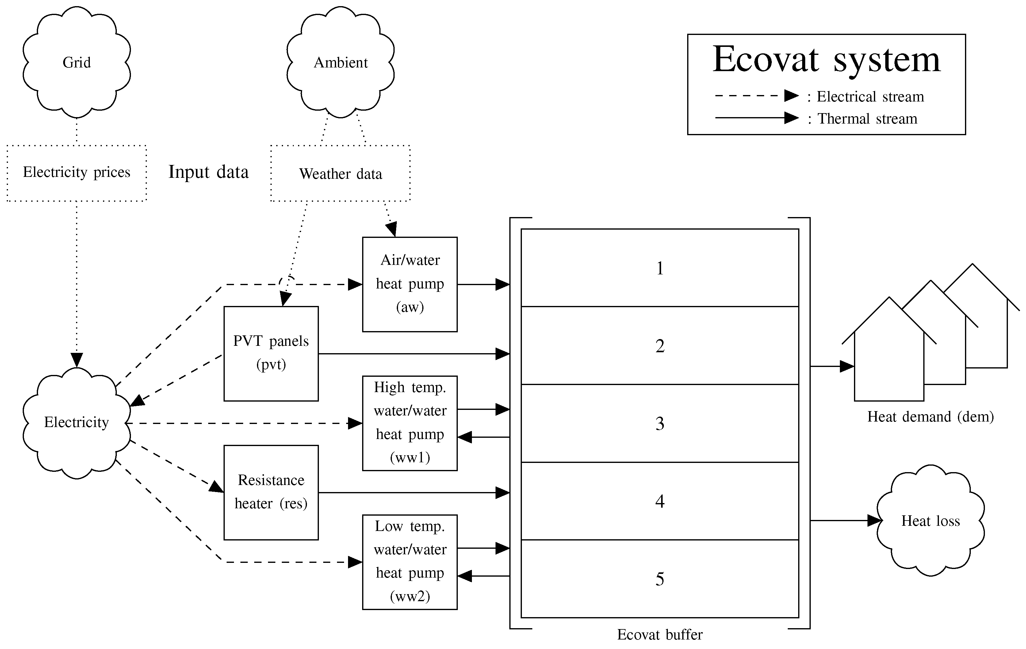
2. Model
2.1. Decision Variables
2.2. PVT Panels
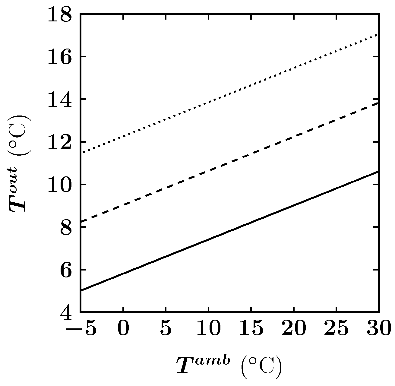
2.3. Air/Water Heat Pump
2.4. Water/Water Heat Pumps
2.5. Resistance Heater
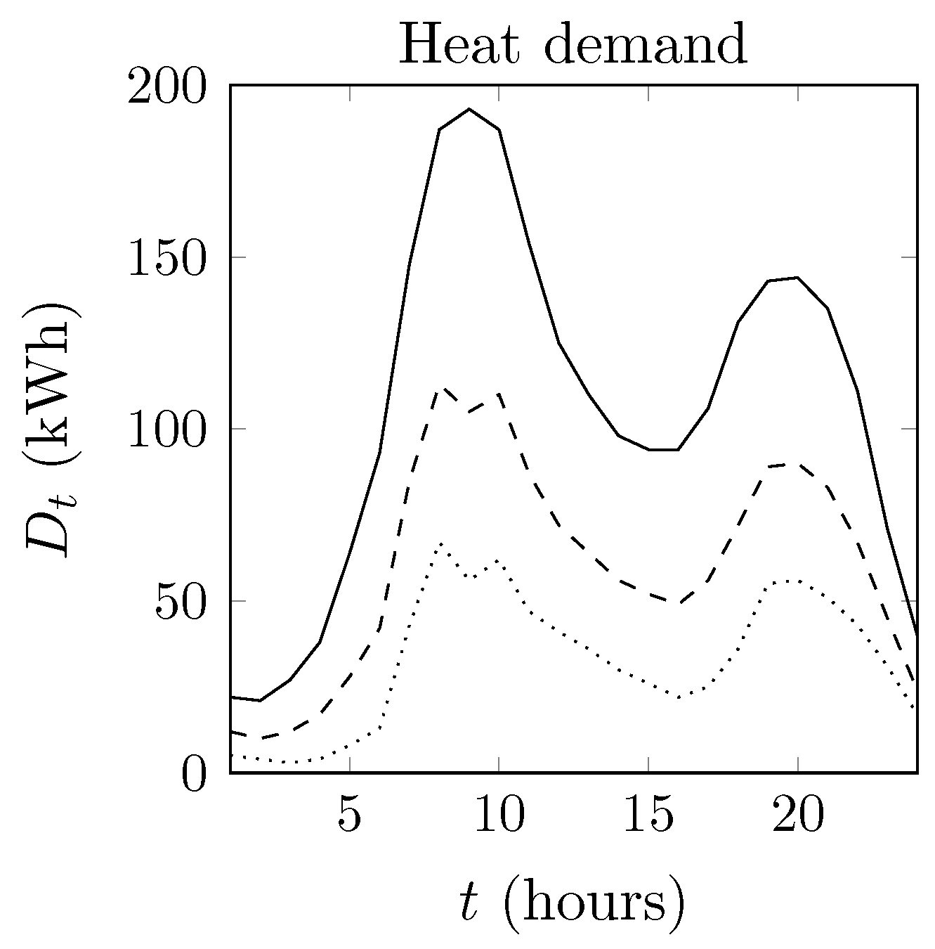
2.6. Heat Demand
2.7. Heat Losses
2.8. Coefficients of Performance
2.9. Temperature Evolution
2.10. Objective Function
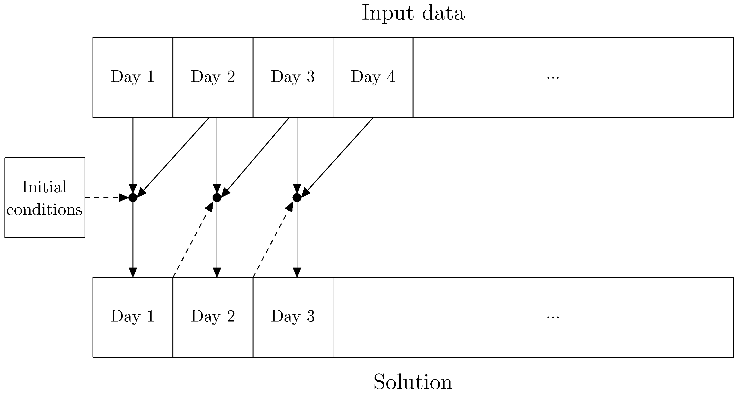
2.11. Summary of the Heuristic Model
3. Optimization Setup
- the gap between the best bound and the best solution found by the solver is less than 0.2 % or
- the solver takes longer than an hour to reach a gap smaller than this percentage.
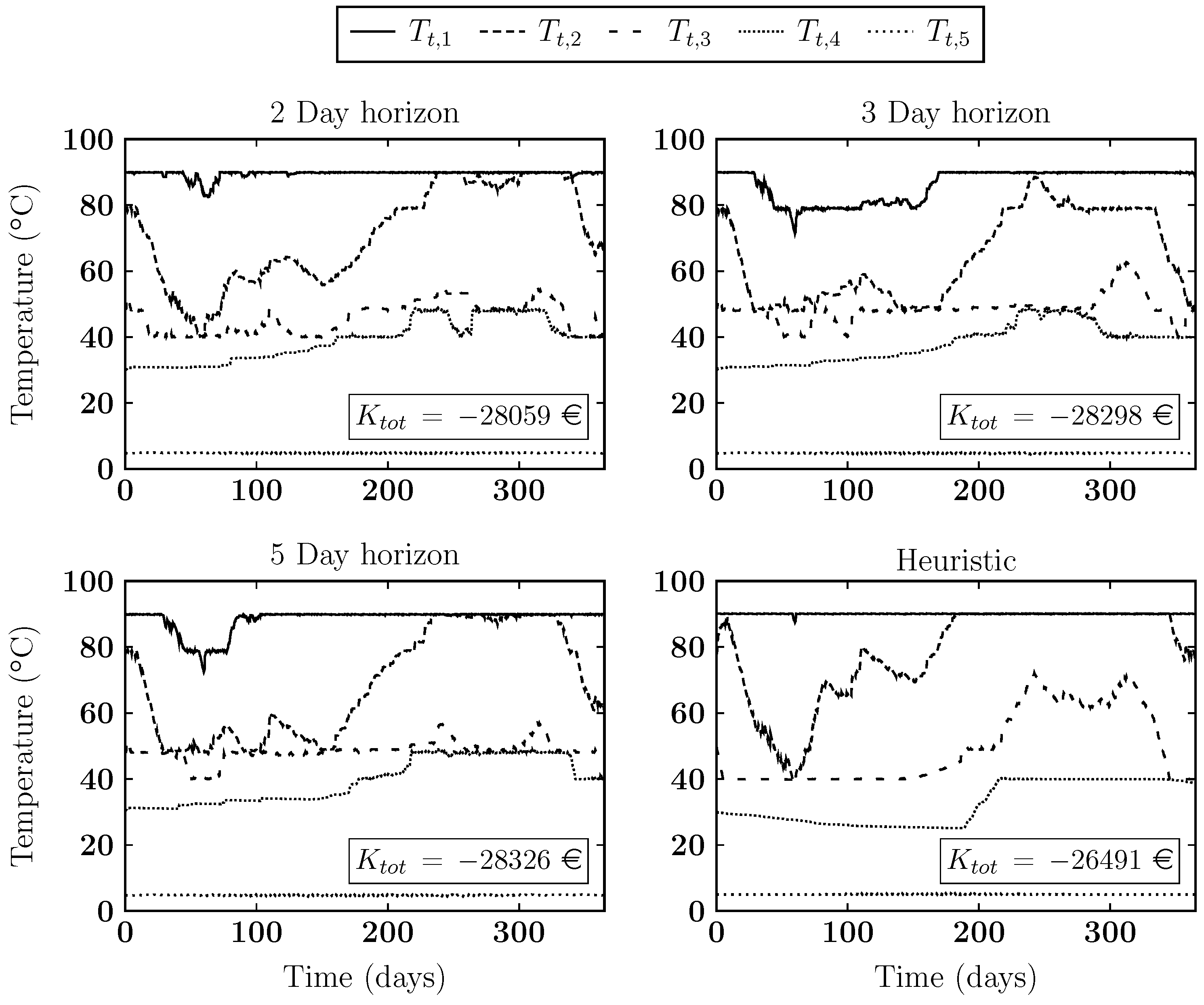
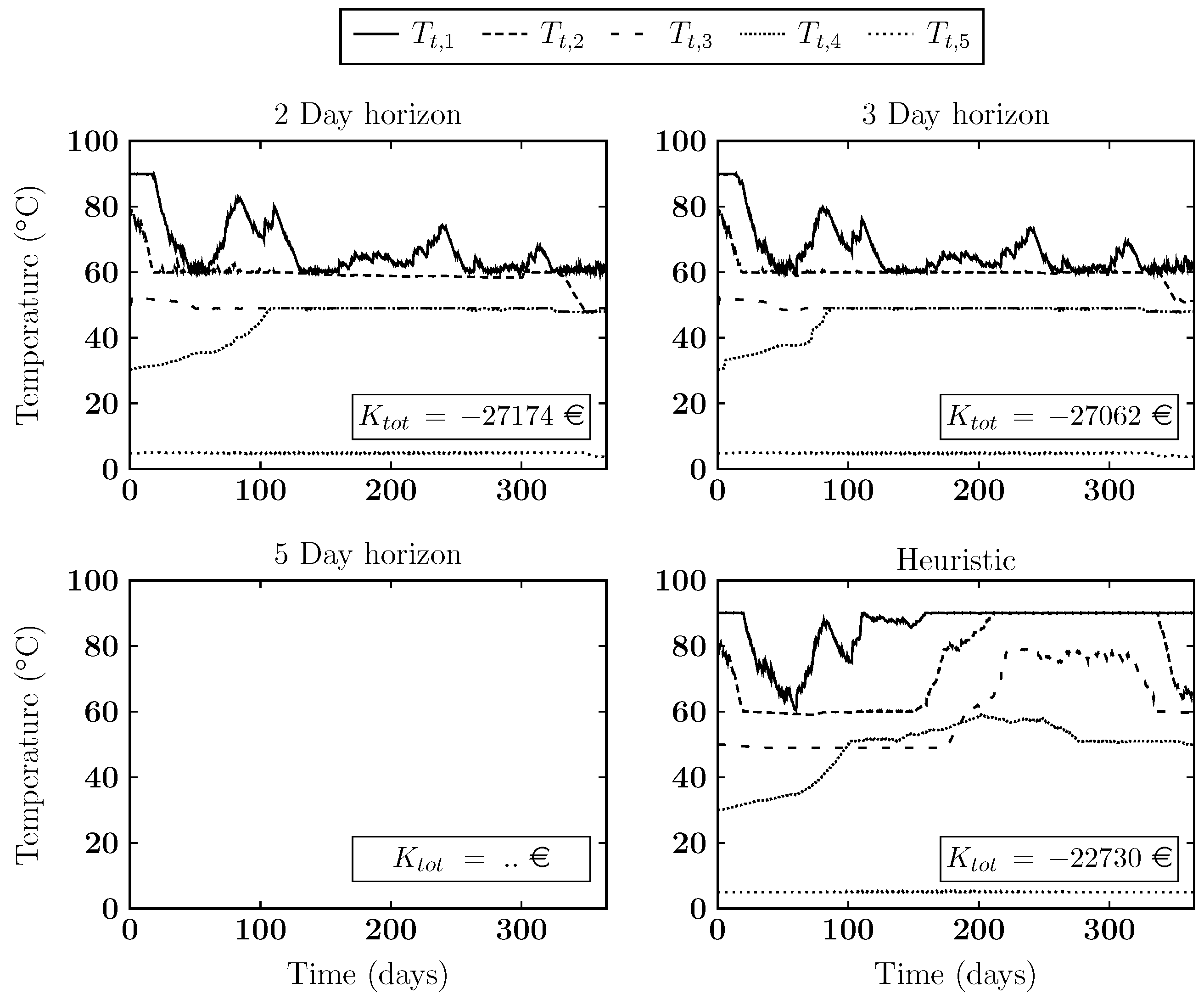
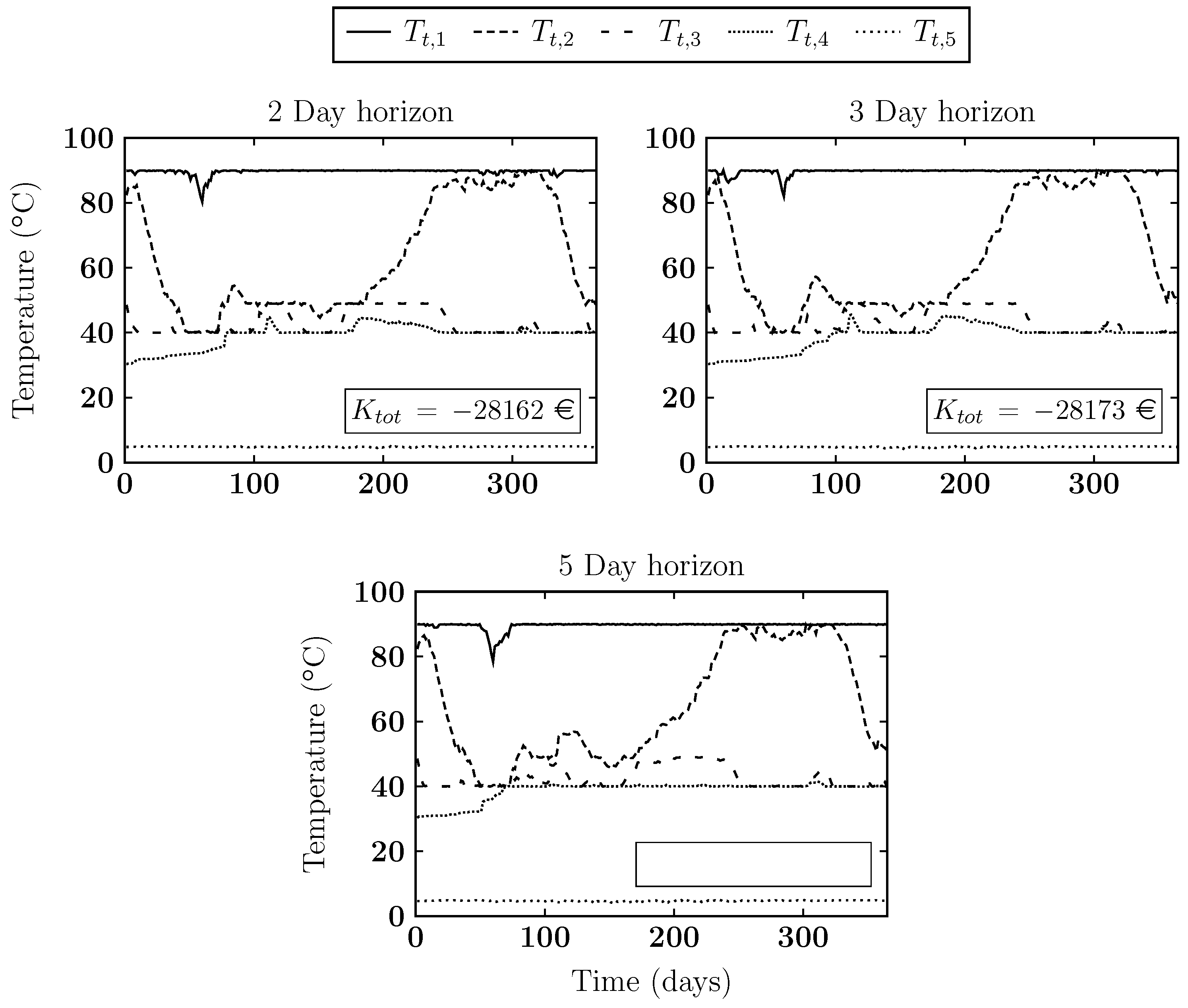
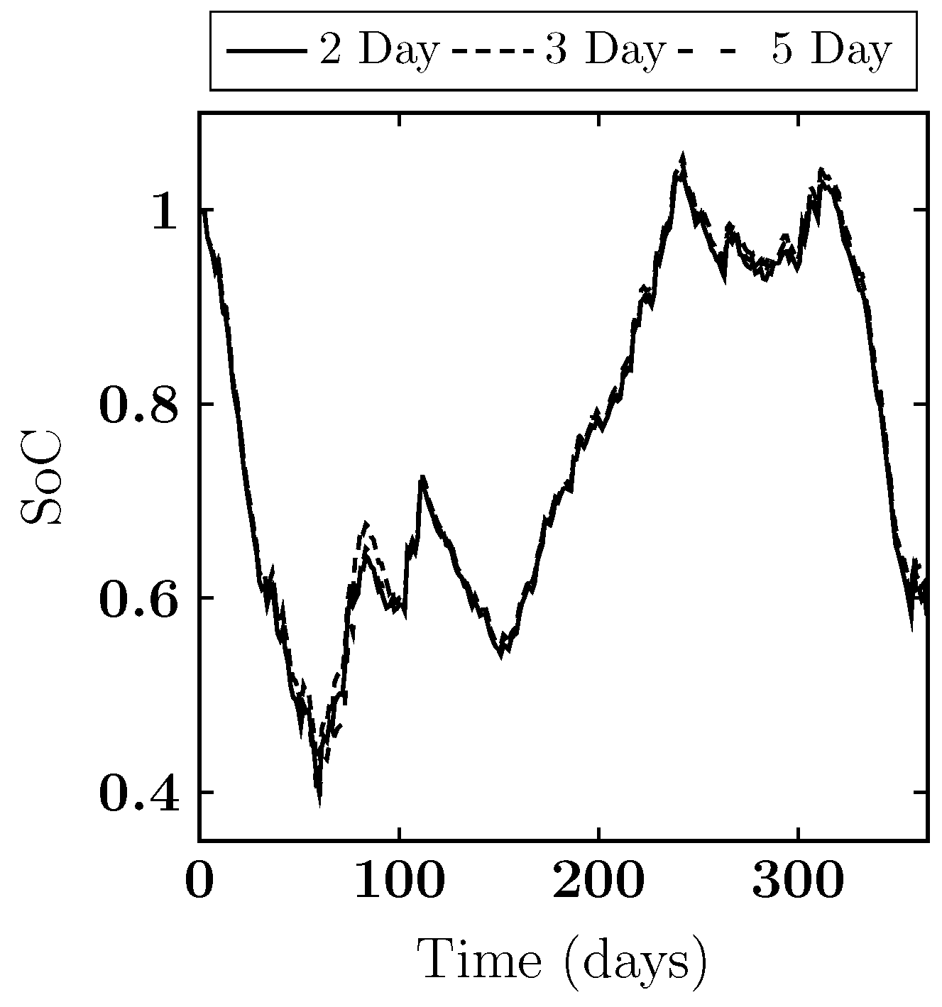
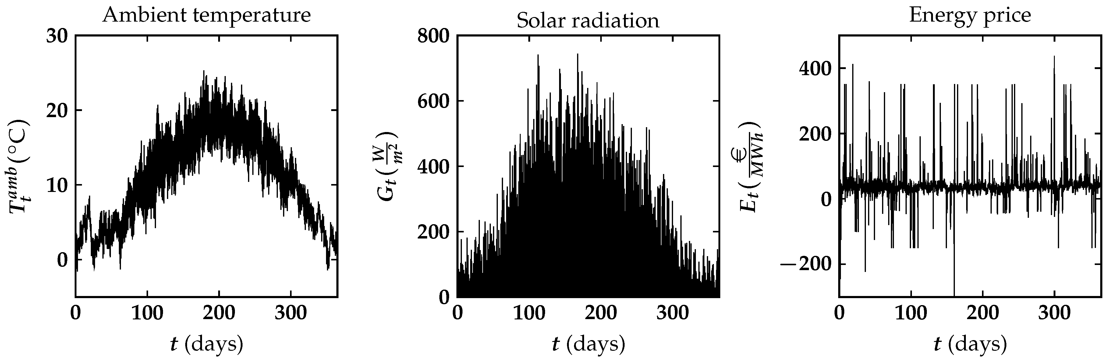
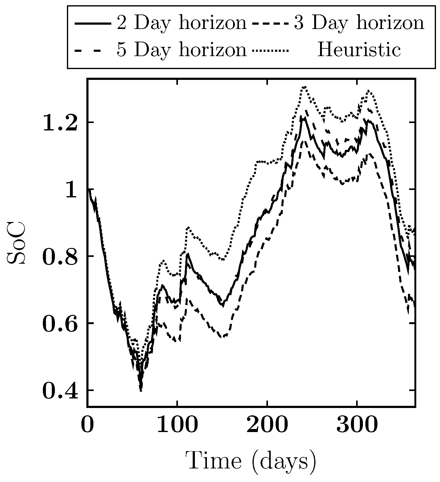
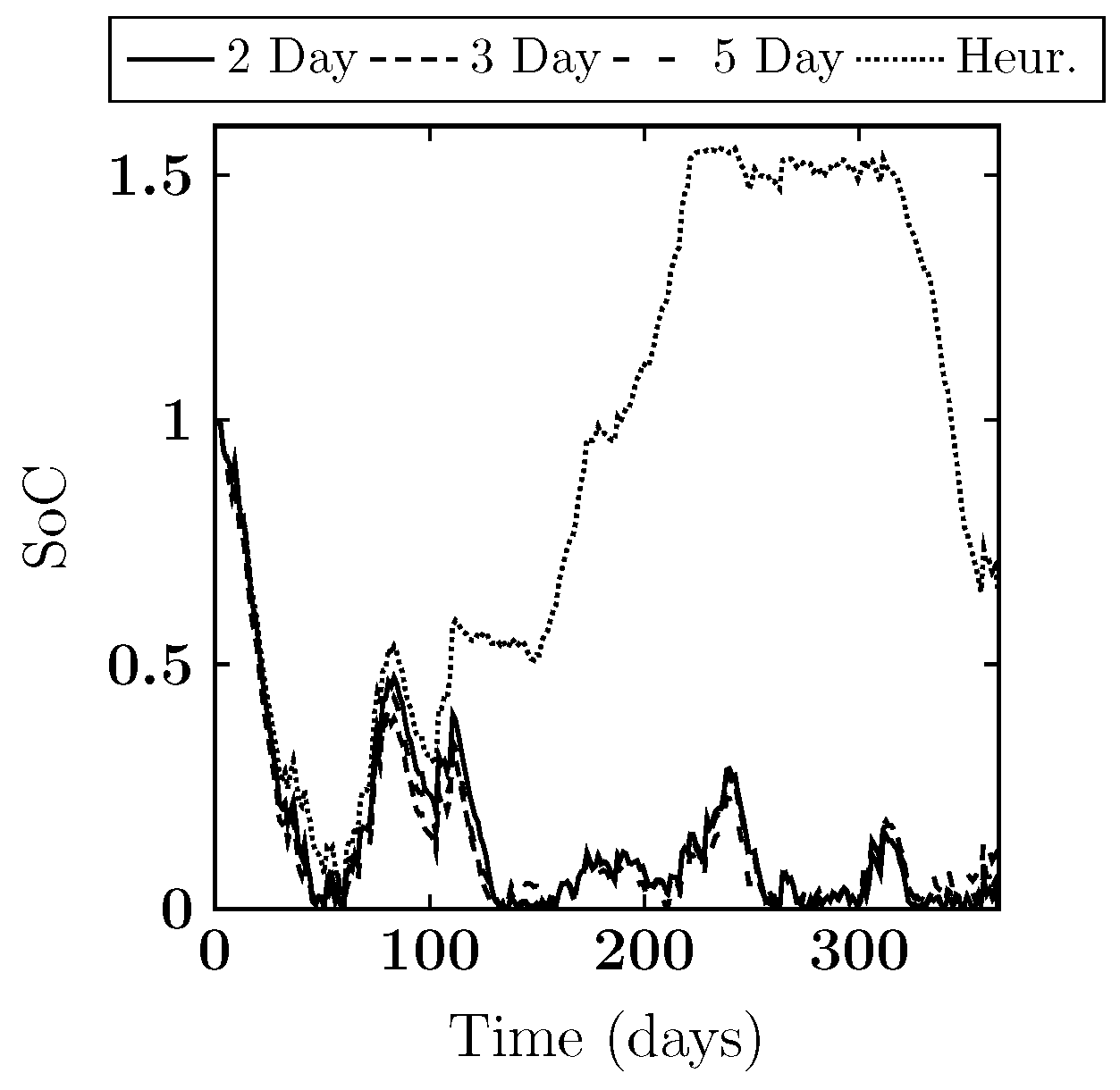
4. Results
5. Conclusions and Future Work
Acknowledgments
Author Contributions
Conflicts of Interest
Nomenclature
Number of segments in the buffer | |
Number of time intervals in the optimization period | |
Length of a time interval | |
Mass of segment s | |
Mass flow rate of the water through the PVT panels | |
Specific heat of water | |
| β | Heat loss factor over 6 months |
Initial temperature distribution in the buffer | |
Demand temperature | |
| , | Minimum and maximum temperatures of the air/water heat pump |
| , , , | Minimum and maximum temperatures of the water/water heat pumps |
Maximum temperature allowed in the buffer | |
Temperature of the ground water | |
Ambient temperature at time t | |
Global radiation at time t | |
Energy price at time t | |
Heat demand at time t | |
Area of panel of the PVT panel | |
Number of PVT panels | |
Thermal efficiency of the PVT panels at a reduced temperature of zero | |
Maximum thermal efficiency of the PVT panels | |
Thermal loss coefficient of the PVT panels | |
Electrical efficiency of the PVT panels at a reduced temperature of zero | |
Maximum electrical efficiency of the PVT panels | |
Electrical loss coefficient of the PVT panels | |
Amount of electrical energy consumed by the air/water heat pumped if turned on | |
| , | Amount of electrical energy consumed by the water/water heat pumps if turned on |
Amount of electrical energy consumed by the resistance heater if turned on | |
Coefficient of performance of the air/water heat pump | |
| , | Coefficients of performance of the water/water heat pumps |
| , | Small constants used in the objective function |
| M | Large constant used in some constraints |
Temperature in segment s at time t | |
Decision variable indicating whether the PVT panels are connected to the bottom segment of the buffer at time t | |
Decision variable indicating whether the air/water heat pump is connected to segment s at time t | |
| , | Decision variables that indicate whether segment s is used as heat source for one of the water/water heat pumps at time t |
| , | Decision variables that indicate whether segment s is used as heat sink for one of the water/water heat pumps at time t |
Decision variable indicating whether the resistance heater is connected to segment s at time t | |
Decision variable indicating whether segment s is supplying the heat demand at time t | |
Indicates whether the output temperature of the PVT panels has a high enough temperature to charge the buffer | |
Input temperature of the PVT panels | |
Output temperature of the PVT panels | |
Reduced temperature | |
| , | Indicate which constraints for the thermal and electrical efficiencies respectively are active |
Energy lost to the surroundings by segment s at time t | |
Energy added to the buffer by the PVT panels at time t | |
Energy added to segment s at time t by the air/water heat pump | |
| , | Energy added to segment s at time t by one of the water/water heat pumps |
| , | Energy extracted from segment s at time t by one of the water/water heat pumps |
Energy added to segment s at time t by the resistance heater | |
Energy extracted from segment s to supply the heat demand at time t | |
Cost of the system at time t | |
Total cost of the system over the optimization period |
References
- Dincer, I.; Rosen, M. Thermal Energy Storage. Systems and Applications; John Wiley & Sons Ltd.: Chichester, UK, 2002. [Google Scholar]
- Dincer, I. On thermal energy storage systems and applications in buildings. Energy Build. 2002, 34, 377–388. [Google Scholar] [CrossRef]
- Arteconi, A.; Hewitt, N.; Polonara, F. State of the art of thermal storage for demand-side management. Appl. Energy 2012, 93, 371–389. [Google Scholar] [CrossRef]
- Xu, J.; Wang, R.; Li, Y. A review of available technologies for seasonal thermal energy storage. Sol. Energy 2014, 103, 610–638. [Google Scholar] [CrossRef]
- Oliveski, R.; Krenzinger, A.; Vielmo, H. Comparison between models for the simulation of hot water storage tanks. Sol. Energy 2003, 75, 121–134. [Google Scholar] [CrossRef]
- Rahman, A.; Smith, A.; Nelson, F. Performance modeling and parametric study of a stratified water thermal storage tank. Appl. Therm. Eng. 2016, 100, 668–679. [Google Scholar] [CrossRef]
- Beniwal, R.; Singh, R.; Saxena, N.S. Thermal storage and investigation on a laboratory solar pond. Heat Recovery Syst. 1984, 4, 401–406. [Google Scholar] [CrossRef]
- Dickinson, J.; Buik, N.; Matthews, M.; Snijders, A. Aquifier thermal energy storage: Theoretical and operational analysis. Géotechnique 2009, 59, 249–260. [Google Scholar] [CrossRef]
- Lavan, Z.; Thompson, J. Experimental study of thermally stratified hot water storage tanks. Sol. Energy 1977, 19, 519–524. [Google Scholar] [CrossRef]
- Rosen, M. The exergy of stratified thermal storages. Sol. Energy 2001, 71, 173–185. [Google Scholar] [CrossRef]
- Han, Y.; Wang, R.; Dai, Y. Thermal stratification within the water tank. Renew. Sustain. Energy Rev. 2009, 13, 1014–1026. [Google Scholar] [CrossRef]
- Hänchen, M.; Brückner, S.; Steinfeld, A. High-temperature thermal storage using a packed bed of rocks—Heat transfer analysis and experimental validation. Appl. Therm. Eng. 2011, 31, 1798–1806. [Google Scholar] [CrossRef]
- Heller, L.; Gauché, P. Modeling of the rock bed thermal energy storage system of a combined cycle solar thermal power plant in South Africa. Sol. Energy 2013, 93, 345–356. [Google Scholar] [CrossRef]
- Sharma, A.; Tyagi, V.; Chen, C.; Buddhi, D. Review on thermal energy storage with phase change materials and applications. Renew. Sustain. Energy Rev. 2009, 13, 318–345. [Google Scholar] [CrossRef]
- Zhou, D.; Zhao, C.; Tian, Y. Review on thermal energy storage with phase change materials (PCMs) in buildings applications. Appl. Energy 2012, 92, 593–605. [Google Scholar] [CrossRef]
- Yan, T.; Wang, R.; Li, T.; Wang, L.; Fred, I. A review of promising candidate reactions for chemical heat storage. Renew. Sustain. Energy Rev. 2015, 43, 13–31. [Google Scholar] [CrossRef]
- Bosch, R. Modelling the Effects of Different Renovation Scenarios of Apartments on the Configuration of the Ecovat Energy Storage System. Master’s Thesis, Technische Universiteit Eindhoven, Eindhoven, The Netherlands, 2015. [Google Scholar]
- Ecovat Renewable Energy Technologies BV. Available online: http://www.ecovat.eu (accessed on 29 April 2016).
- Zondag, H. Flat-plate PV-Thermal collectors and systems: A review. Renew. Sustain. Energy Rev. 2008, 12, 891–959. [Google Scholar] [CrossRef]
- Kim, J.H.; Kim, J.T. Comparison of electrical and thermal performances of glazed and unglazed PVT collectors. Int. J. Photoenergy 2012, 2012, 957847. [Google Scholar] [CrossRef]
- Dupeyrat, R.; Ménézo, C.; Fortuin, S. Study of the thermal and electrical performances of PVT solar hot water system. Energy Build. 2014, 68, 751–755. [Google Scholar] [CrossRef]
- Williams, H. Model Building in Mathematical Programming, 5th ed.; John Wiley & Sons Ltd.: Chichester, UK, 2013. [Google Scholar]


| Input Parameters Ecovat System | |||
|---|---|---|---|
| Parameter | Value | Parameter | Value |
| 5 | 1.8 | ||
| 35,040 | 83 | ||
| 900 s | 0.73 | ||
| {1.04, 1.04, 1.04, 9.11, 9.11 kg | 0.75 | ||
| 7.25 | |||
| 0.018 kg/s | 0.1 | ||
| 4168 J/(kg K) | 0.15 | ||
| β | 0.08 | 0.44 | |
| °C | 9 kW | ||
| 40 or 60 °C | 15 kW | ||
| 0 °C | 15 kW | ||
| 59 °C | 1000 kW | ||
| 0 °C | 2.686 | ||
| 49 °C | 2.851 | ||
| 48 °C | 3.681 | ||
| 79 °C | 1 | ||
| 90 °C | 1 | ||
| 15 °C | M | 150 | |
© 2016 by the authors; licensee MDPI, Basel, Switzerland. This article is an open access article distributed under the terms and conditions of the Creative Commons Attribution (CC-BY) license (http://creativecommons.org/licenses/by/4.0/).
Share and Cite
De Goeijen, G.J.H.; Smit, G.J.M.; Hurink, J.L. An Integer Linear Programming Model for an Ecovat Buffer. Energies 2016, 9, 592. https://doi.org/10.3390/en9080592
De Goeijen GJH, Smit GJM, Hurink JL. An Integer Linear Programming Model for an Ecovat Buffer. Energies. 2016; 9(8):592. https://doi.org/10.3390/en9080592
Chicago/Turabian StyleDe Goeijen, Gijs J. H., Gerard J. M. Smit, and Johann L. Hurink. 2016. "An Integer Linear Programming Model for an Ecovat Buffer" Energies 9, no. 8: 592. https://doi.org/10.3390/en9080592
APA StyleDe Goeijen, G. J. H., Smit, G. J. M., & Hurink, J. L. (2016). An Integer Linear Programming Model for an Ecovat Buffer. Energies, 9(8), 592. https://doi.org/10.3390/en9080592