Article

Optimal Cooling Load Sharing Strategies for Different Types of Absorption Chillers in Trigeneration Plants

Department of Mechanical Engineering, University Rovira i Virgili, CREVER-Research Group on Applied Thermal Engineering, Avda. Països Catalans 26, Tarragona 43007, Spain
*
Author to whom correspondence should be addressed.
Energies 2016, 9(8), 573; https://doi.org/10.3390/en9080573
Submission received: 16 March 2016 / Revised: 8 July 2016 / Accepted: 11 July 2016 / Published: 25 July 2016
(This article belongs to the Special Issue Simulation of Polygeneration Systems)

Abstract

:
Trigeneration plants can use different types of chillers in the same plant, typically single effect and double effect absorption chillers, vapour compression chillers and also cooling storage systems. The highly variable cooling demand of the buildings connected to a district heating and cooling (DHC) network has to be distributed among these chillers to achieve lower operating costs and higher energy efficiencies. This problem is difficult to solve due to the different partial load behaviour of each chiller and the different chiller combinations that can cover a certain cooling demand using an appropriate sizing of the cooling storage. The objective of this paper is to optimize the daily plant operation of an existing trigeneration plant based on cogeneration engines and to study the optimal cooling load sharing between different types of absorption chillers using a mixed integer linear programming (MILP) model. Real data from a trigeneration plant connected to a DHC close to Barcelona (Spain) is used for the development of this model. The cooling load distribution among the different units is heavily influenced by the price of the electricity sold to the grid which rules the duration of the operation time of the engines. The main parameter to compare load distribution configurations is the primary energy saving indicator. Cooling load distribution among the different chillers changes also with the load of the whole plant because the chiller performance changes with load.

Graphical Abstract

1. Introduction and Objectives

Trigeneration plants integrated into district heating and cooling (DHC) networks are a very efficient way to provide energy services with the exploitation of locally generated waste heat to produce heating and cooling in a very efficient way and delivering them to final users. In this way the users benefit from a scale factor with respect to the efficiency of the energy supply systems, avoid the cost of maintenance and save precious space in their facilities as the main advantages. Other more general and very important benefits are related with the saving of primary energy and lower environmental impact [1]. In many cases the deployment of DHC networks is not as fast as initially planned at the design stage of the project because the number of consumers connected to the DHC increases at a slower pace than expected. Trigeneration plants connected to DHC networks are designed to operate in several modules of cogeneration engines that can be connected and disconnected to the system to account for this type of problems and the variability of the users demand. In many cases, modularity and flexibility of modern and efficient trigeneration plants is not enough to properly work at the very low partial load when serving the DHC during the first stages of the implementation of the project [2]. A low load of the plant can lead to low energy efficiency.
Additionally trigeneration plants can use different types of units, typically single effect and double effect absorption chillers, vapor compression chillers and cooling storage systems. The variable cooling load demand of the buildings connected to the DHC has to be distributed among these chillers to achieve lower operating costs and higher energy efficiencies. This problem is even more difficult to solve taking into account the different partial load behavior of each chiller and the high number of possible unit combinations that can cover a given demand specially with the appropriate dimensioning of the cooling storage.
The distribution of the load or “load sharing” should not be confused with the load sharing concept also used in the literatures [3,4] that refers to a system with a thermal and/or cooling load from a diversified type of end users (residential and commercial users and different types of industries). This last definition could be regarded as an “external load sharing”. In this case the overlapping of the load demand is interesting to increase the trigeneration plant efficiency due to a higher number of annual operation hours. Piacentino et al. [5] presented one of these cases where a comprehensive tool is presented for the optimization of polygeneration systems serving a group of different types of buildings.
Another concept is the “internal load sharing” inside of the trigeneration plant between the units providing the same type of utility, electricity, heating or cooling. This last concept is of special interest to develop the load-sharing strategy to maximize the aggregate performance [6]. In this paper both external and internal load sharing will be considered but only the internal cooling load sharing will be studied.
Usually, multiple-chillers systems are controlled using a sequential approach to provide the building load demand [7]. Since the flow of chilled water in each chiller is constant and the chilled water temperature provided by each chiller has to be the same, they have to operate at the same part load ratio. Instead of this it could be interesting to study other sharing load strategies. Abou-Ziyan and Alajmi [6] analysed the load sharing effect in multiple reciprocating compression chillers and sharing the load between the four compressors that equipped each compression chiller. It was reported a performance improvement between 22% and 33% with respect to the same part load ratio distribution strategy. Yu and Chan [8] studied the load distribution between chillers of equal or different sizes. They propose to use the maximum load in one of them and the other running at partial load. In the case of different sizes, the biggest one should be kept at full capacity and the other one will follow the load. These preliminary strategies can be used applied in compression chillers but are not of direct application for absorption chillers that are not only affected by their own partial load characteristics, ambient conditions and variability of the load demand but also by additional effects, such as the characteristics of the waste heat use to drive the system. Underwood et al. [9] studied the simultaneous chilled water demand distribution between a single effect absorption chiller and a compression chiller in a theoretical case study. The conclusion was that this arrangement could be of interest when the power demand is lower than the rated capacity of the cogeneration plant and the cooling demand is high. Energy costs were not considered in this study.
Many studies have been carried out such as Hajabdollahi et al. [10], Chicco and Mancarella [11] and Stojiljkovic et al. [12], just to mention a few, to optimize the operation and/or design of trigeneration plants using partial load characteristics and different optimization approaches and objectives [13] including in some cases thermoeconomic and exergy analysis [14] or environmental information obtained through life cycle analysis techniques incorporated into the optimization model [15]. In some cases the main interest is focused in the design of new trigeneration systems for DHC networks for different cases such as big urban areas [16], for small scale applications with the integration of renewable energy sources [17] or to study the combined effect of optimized energy supply systems and reduction of home energy demands [18]. Many of all these studies include operational optimization but are more focused on the design because the partial load behaviour of the units is generic and do not correspond to any specific equipment. Then, no distinction can be made on different types of thermal chillers.
However, the number of studies in literature based on real data from trigeneration plants connected to a DHC is very scant. Thus it is clear that the current literature lacks empirical or operational data to validate thermodynamic models of integrated systems with multiple components [9,13]. Also there is no information on the actual energy efficiency of trigeneration plants working at low partial load. Even the information on the performance at partial load of some key components such as absorption chillers is more limited that it could be expected. The abundant information available comes mainly from manufacturer’s data or laboratory tests of low capacity chillers [19,20,21] instead of on-site field measurements during plant operation.
So far the load sharing optimization has not been studied for a combination of different types of chillers (thermally driven and compression chillers) and connected to a cooling storage. This paper presents a mixed integer linear programming (MILP) model of a trigeneration plant based on cogeneration engines. MILP has been proposed and utilized widely as one of the most effective optimization approaches for this type of problems [22,23]. It leads to a natural expression of decision variables. For example, the selection, number, and on/off status of operation of equipment are expressed by integer variables and the capacities and load allocation of equipment by continuous ones. This model is used to optimize the daily plant operation and to study the optimal cooling load sharing between the different types of absorption chillers, compression chillers and cooling storage. The main parameter to compare load distribution configurations will be the primary energy saving. The heat of the exhaust gases is recovered to produce cooling in a double effect chiller and the engine cooling waste heat is used to drive a single effect absorption chiller. A high efficiency compression chiller is used as a back-up system. The system uses also a chilled water storage tank. Real data from a trigeneration plant connected to a DHC close to Barcelona (Spain) is used for the development of the model. A second objective of the paper is to study the efficiency of this type of trigeneration plants working at cooling load demands lower that 50% of its nominal capacity.

2. Description of the Trigeneration Plant

In the framework of the Polycity project [24] a high efficiency energy polygeneration plant was implemented in a new urban development called Parc de l’Alba in Cerdanyola del Vallès (Barcelona, Spain). This area includes a science and technology park with a Synchrotron light facility called ALBA as well as other low energy consumption buildings. This project was executed in several stages. In a first stage, it was built a trigeneration plant known as ST-4 based on cogeneration engines. In the next stages of the project is expected to increase the number of engines and chillers in service and probably the integration of renewable energy sources. Ortiga et al. [2] presented the initial design of this new plant under different scenarios (development stages, integration of renewables, costs, etc.). The CREVER research group at the Universitat Rovira i Virgili in Tarragona (Spain) is monitoring this trigeneration plant in order to evaluate its performance using current operation data and propose new operation strategies and possible energy saving measures. The process data analysed corresponds to the energy production in summer 2014.

2.1. Main Components

The ST-4 plant provides electricity, hot and chilled water for a synchrotron light facility and other buildings which belong to the Science and Technology Park called Alba Park using a four pipe DHC network. 
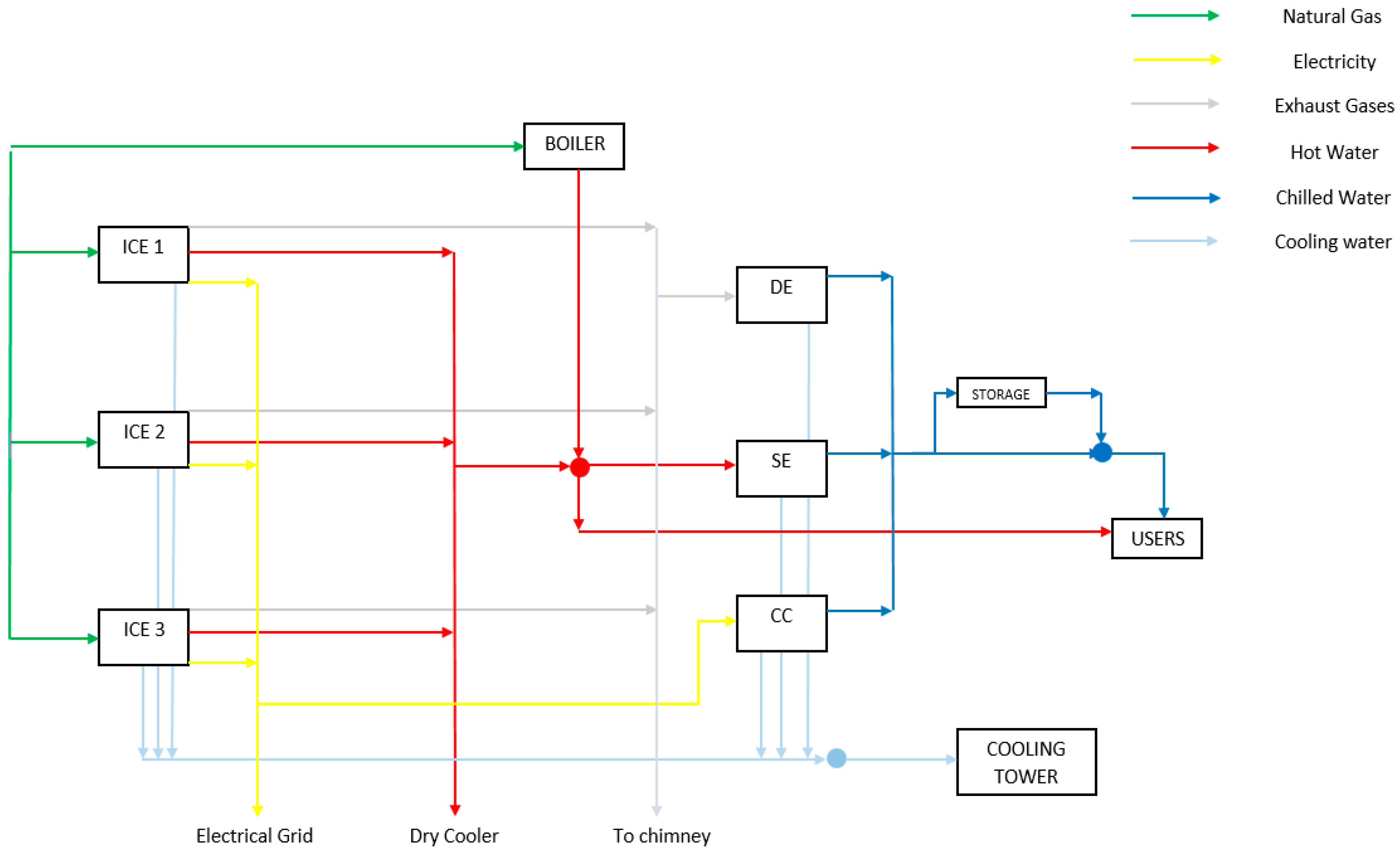
Figure 1 shows the system configuration with their main components and energy streams. The main customer of the DHC network is the ALBA synchrotron light source facility that includes the laboratory and office building. The nominal capacity required is 8750 kW and 1400 kW for cooling and heating, respectively. This facility requires cooling at 7.0 ± 0.5 °C for heating, ventilation and air conditioning (HVAC), Deionized water at 23.0 ± 0.2 °C to remove the heat load from the synchrotron light source, and hot water at 50.0 ± 1 °C and operates more than 5000 h/year considering the maintenance activities. Therefore, the demand of cooling and heating from the trigeneration plant is guaranteed.
The main units of the plant are three turbocharged cogeneration engines (JMS 620 GS-N.L, GE Jenbacher GmbH & Co., Jenbach, Austria) with intercooler based on the Miller cycle, and a unitary electrical nominal capacity of 3354 kW and 3102 kW of total thermal energy if the exhaust gases are cooled down to 120 °C. The nominal electrical efficiency is 45% and the global thermal efficiency is 86.5%. The exhaust gases of these engines are used to drive a 5 MW series flow double effect water/LiBr ED 80C CX absorption chiller (Thermax Limited, Chinchwad, India). This chiller has a two stage evaporator (twin design concept) that produces a higher temperature difference in the chilled water in order to reduce the mass flow circulation and at the same time increases the coefficient of performance (COP). The heat recovered from the jacket cooling system of the cogeneration engines is used to drive a 3 MW single effect absorption chiller (Thermax LT 105T) based on the twin design concept. A twin design of the low pressure components evaporator/absorber and the high pressure components generator/condenser are of interest to cope with a large temperature difference between the inlet and outlet of the external heat carriers [25] as is the most suitable situation in chillers connected to DHC networks. It is also interesting for the chiller capacity regulation because it depends not only on the temperature of the external heat sources but also on their temperature difference [26].
Chilled water can be produced also using a 5 MW 19XR 8587 compression chiller (Carrier Co., Syracuse, NY, USA) equipped with a hermetic centrifugal compressor and a variable speed drive. A natural gas fired-tube boiler of 5 MW is available as backup for heating. There is also a chilled water storage of 4000 m3 to deliver about 7 MW of cooling during 2.5 h for a temperature difference of 6 °C. The interested reader can refer to Ortiga et al. [2] for a more detailed description of the plant and the performance of their components in nominal conditions.

2.2. Monitoring System

The entire system is monitored and controlled by sensors of temperature, flow rate and thermal energy meters. A data acquisition system has been connected to the supervisory, control and data acquisition (SCADA) system of the ST-4 plant to collect specific data of interest for the energy analysis of the plant. The process variables are registered each minute and stored. Nowadays data acquisition system can record multiple variables in short sampling times. As result, the volume of information available is very large and it might be difficult to calculate mass and energy balance. These balances may not be met due to: random and gross errors in the measurements, deviations from steady state, redundancy in the measurements, etc. Therefore the methodologies used for the data treatment should generate a coherent set of measurements so the performance of the absorption chillers can be reliably estimated [21].

2.3. Monitored Data and Operation Schedule

The most singular units in the plant for its special design (Section 2.1) are the two absorption chillers. Table 1 and Table 2 show some stationary working conditions for both chillers in different dates.
All the variables correspond to the external circuits because there is no information on internal parameters as it is the usual situation for industrial applications. Each column corresponds to a certain period for one day. The first column of data (NC) refers to the values of the same unit at nominal conditions to compare with the working conditions of a certain period of day. Q losses correspond to the discrepancy in the global energy balance of the unit due to usual deviation in steady-state, measuring instruments, etc. The main lessons that could be extracted from these data is the capacity of the chillers to work well below its nominal capacity and the wide temperature of the hot water and exhaust gases used to drive the chillers. The data presented in Figure 2 and Figure 3 show that the COP of the single- and double-effect chillers is reasonably acceptable in spite of the low cooling load of the plant, between 0.6–0.65 and close to 1, respectively for a load around 40% of its nominal capacity.
Typically during weekdays the three engines are running at full capacity, from 8 h to 23 h, to take advantage of high price of electricity during this period. Some weeks in July and August only two engines produce electricity because of the decrease in the energy demand. During the night and weekends are usually out of service also due to the low price of electricity in these periods.
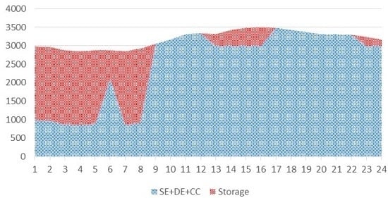
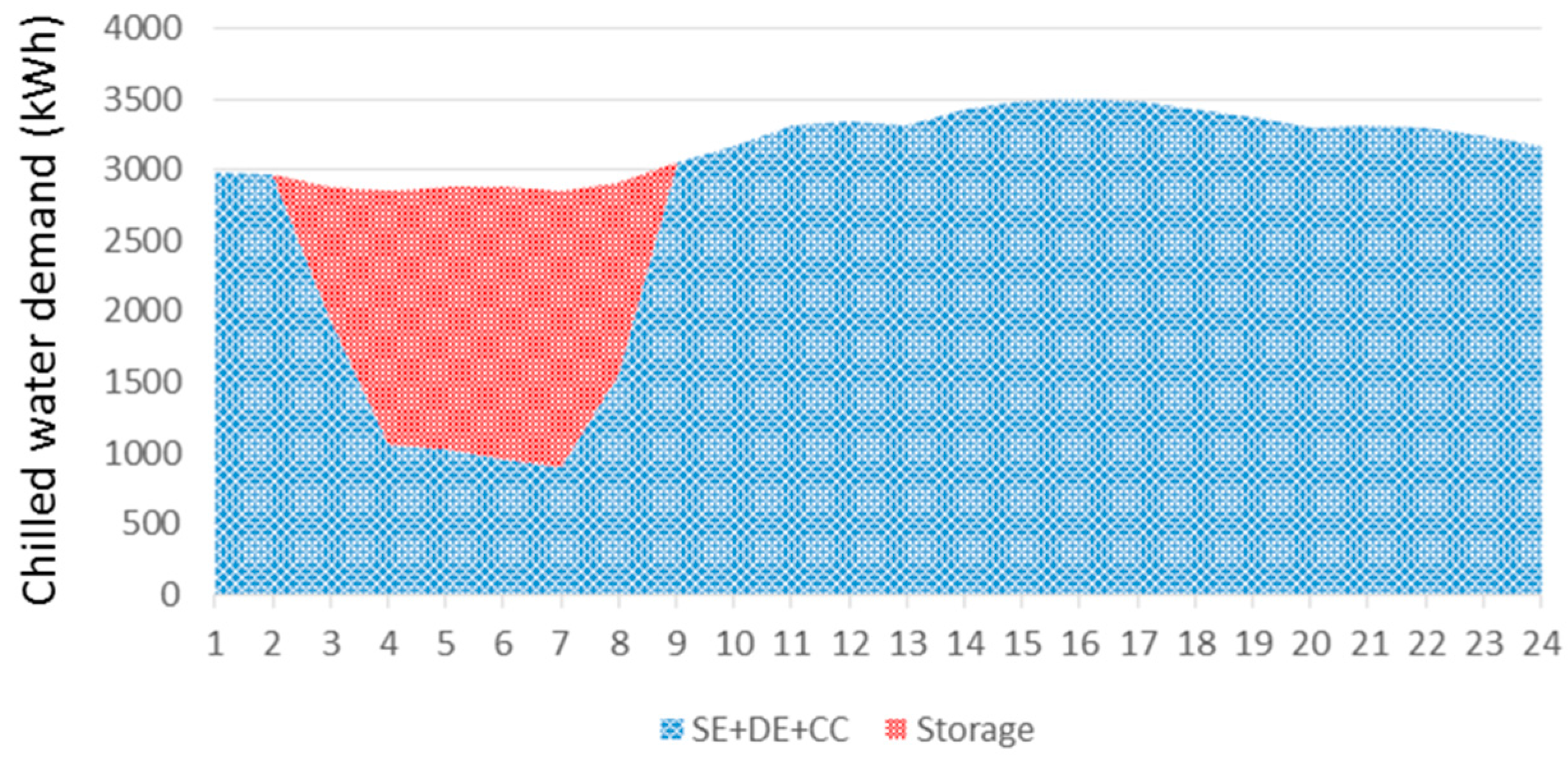
The required thermal energy for the DHC network during the weekend is supplied by the gas boiler. In emergency cases the heat provided by the boiler could substitute one of the engines if required. However, the thermal chillers are only working when the engines are in operation. In this period, the chilled water storage is in recharge mode.
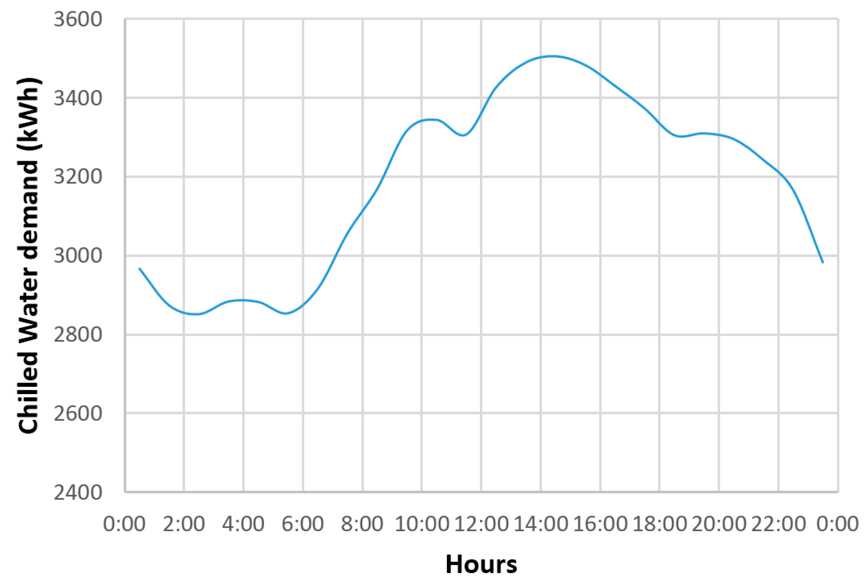
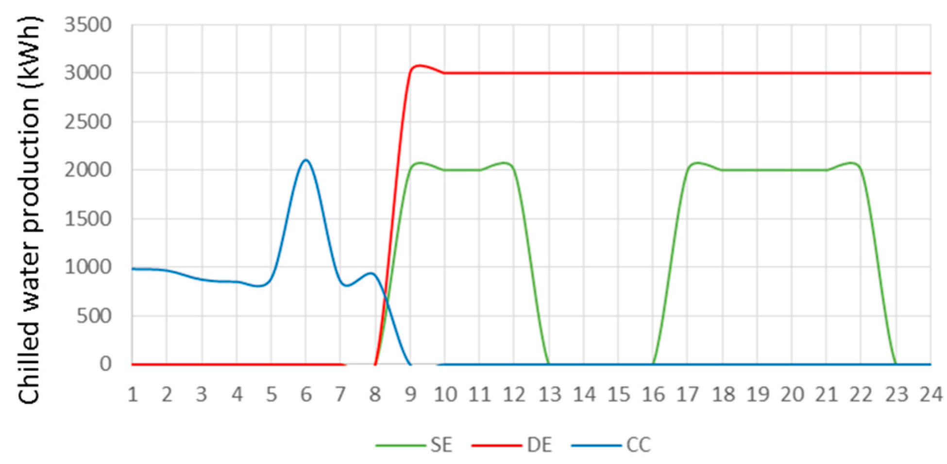
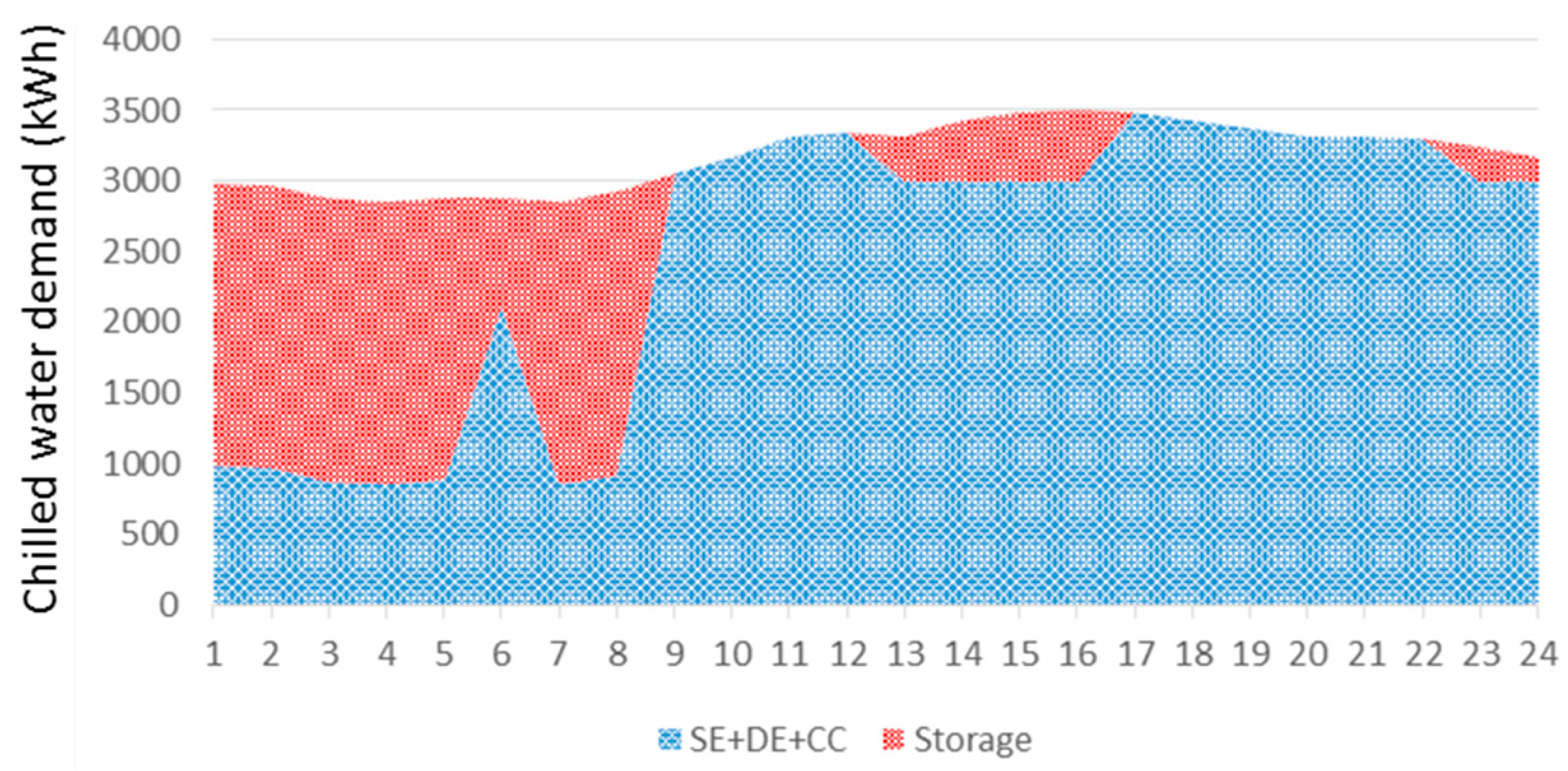
The present demand of chilled water in summer is covered by the single- and DE absorption chillers at partial load (usually not higher than 50%). During the night (approximately from 23 h to 8 h) and weekend periods the cooling demand is covered using the compression chiller and the cooling storage system. During the night, the preferred system is the cooling storage and during the weekend is the compression chiller.

3. Modelling

The mathematical programming optimization model was developed using general algebraic modelling system (GAMS) with the solver Cplex. The model is able to optimize the operational strategy for a typical day using a MILP approach. The binary variables are used to indicate when a given unit is in operation or not, o when the storage tank changes its operation mode. The objective function (Equation (1)) is the difference between the income to the plant (Equation (2)) and the operational (Equation (3)) and maintenance costs. In this model i stands for a given unit and j is the time period (one hour). Electricity sold to the grid is calculated through the balance presented in Equation (4), CCEl is the electricity for the compression chiller, CTfans for the cooling tower fans, ElDryCooler for rejecting heat from the engines cooling system, Elpumps for all the plant pumps and Elventilation for the rejection of heat from the engines’ rooms. This last value has been considered to be of 74 kW per engine in operation:
O b j e c t i v e = I n c o m e C o s t operational C o s t maintenance
I n c o m e = j = 1 24 ( E l to grid ( j ) × E l export price + D e m a n d cooling ( j ) × P r i c e cooling + D e m a n d HW ( j ) × P r i c e HW )
o s t operational = j = 1 24 i = 1 3 I C E fuel ( i , j ) × N G price +   j = 1 24 B o i l e r fuel ( j ) × N G price + j = 1 24 E l from grid ( j ) × E l import price +   j = 1 24 M a k e U p × P r i c e water
i = 1 3 I C E E l ( i , j ) + E l grid ( j ) = E l ICE to grid + C C E l + C T fans + E l DryCooler + E l pumps + E l ventilation

3.1. Engines Constraints

I C E E l ( i , j ) I C E Nominal × I C E on ( i , j )
I C E E l ( i , j ) I C E Minimal Load × I C E Nominal × I C E on ( i , j )
I C E fuel ( i , j ) × I C E eff E l   = I C E E l ( i , j )
I C E ExGas ( j ) =   i = 1 3 I C E fuel ( i , j ) × I C E eff exGas
I C E HW ( j ) =   i = 1 3 I C E fuel ( i , j ) × I C E eff HW
I C E on ( i , j ) I C E on ( i , j 1 ) + I C E on ( i , j + 1 )
I C E on ( i , j ) I C E on ( i , j 1 ) + I C E on ( i , j + 1 ) 1
Equations (10) and (11) are useful to avoid continuous ON-OFF of the engines and impose at least two hours of continuous working. Equivalent constraints are applied for the other units: boiler and absorption and compression chillers.

3.2. Boiler Constraints

B o i l e r capacity ( j ) = B o i l e r eff × B o i l e r fuel ( j )
B o i l e r capacity ( j ) = B o i l e r HW to users ( j ) + B o i l e r HW to  S E ( j )
B o i l e r capacity B o i l e r Nominal Capacity × B o i l e r on ( j )
B o i l e r HW to  S E ( j ) B o i l e r Nominal Capacity × S E on ( j )
H o t Demand ( j ) = I C E HW to users ( j ) + B o i l e r HW to users ( j )
B o i l e r on ( j ) B o i l e r on ( j 1 ) + B o i l e r on   ( j + 1 )
B o i l e r on ( j ) B o i l e r on ( j 1 ) + B o i l e r on ( j + 1 ) 1

3.3. Double Effect Absorption Chiller Constraints

E x G a s Atm ( j ) + Q gen  D E ( j ) = I C E ExGas ( j )
Q eva  D E ( j ) = 1.6235 × Q gen  D E ( j ) 1591.6 × D E on ( j )
Q eva  D E ( j ) D E Minimal Load × D E Nominal Capacity × D E on ( j )
Q eva  D E ( j ) D E Nominal Capacity × D E on ( j )
D E on ( j ) D E on ( j 1 ) + D E on   ( j + 1 )
D E on ( j ) D E on ( j 1 ) + D E on ( j + 1 ) 1

3.4. Single Effect Absorption Chiller Constraints

I C E HW ( j ) = Q gen  S E ( j ) + H W diss ( j ) + I C E HW to users   ( j )
D r y   C o o l e r E l ( j ) = 0.0129 × H W diss ( j ) + 1.83
Q eva  S E ( j ) = 0.0759 × ( Q gen  S E ( j ) + B o i l e r HW to  S E ( j ) ) 247.16 × S E on ( j )
Q eva  S E ( j ) S E Nominal Capacity   × S E on ( j )  
Q eva  S E ( j ) S E Nominal Capacity   × S E Minimal Load × S E on ( j )  
S E on ( j ) S E on ( j 1 ) + S E on   ( j + 1 )
S E on ( j ) S E on ( j 1 ) + S E on ( j + 1 ) 1

3.5. Compression Chiller Constraints

C C capacity ( j ) C C Nominal Capacity × C C on ( j )
C C E l ( j ) = C C capacity ( j ) C O P C C
C C on ( j ) C C on ( j 1 ) + C C on   ( j + 1 )
C C on ( j ) C C on ( j 1 ) + C C on ( j + 1 ) 1

3.6. Storage System Constraints

S t o r a g e in ( j ) + S t o r a g e ByPass ( j ) = Q eva  D E ( j ) + Q eva  S E ( j ) + C C Capacity ( j )
C h i l l   D e m a n d ( j ) = S t o r a g e out ( j ) + S t o r a g e ByPass ( j )
E n e r g y   B a l a n c e ( j ) = S t o r a g e in ( j ) S t o r a g e out ( j )
E n e r g y   L e v e l ( j ) = E n e r g y   L e v e l ( j 1 ) + S t o r a g e in ( j ) + S t o r a g e out ( j )
S t o r a g e in ( j ) 2000 × S t o r a g e on ( j )
S t o r a g e out ( j ) 2000 × ( 1 S t o r a g e on ( j ) )
j = 1 24 y 1 23
E n e r g y   L e v e l ( j ) M a x   L e v e l × y 1

3.7. Cooling Tower Constraints

P E l = Q CT , component 114.2
I C E CT ( j ) =   i = 1 3 370 × I C E on ( i , j )
C T D E ( j ) = ( Q gen  D E ( j ) + Q eva  D E ( j ) ) 114.2
C T S E ( j ) = ( Q gen  S E ( j ) + Q eva  S E ( j ) ) 114.2
C T C C ( j ) = C C capacity ( j ) × C O P C C + 1 C O P C C × 1 114.2
Q CT ( j ) = Q gen  D E   ( j ) +   Q eva  D E ( j ) + Q gen  S E   ( j ) +   Q eva  S E ( j ) + I C E CT ( j ) +   C C capacity ( j ) × C O P C C + 1 C O P C C
m a ( j ) = Q CT ( j ) 10 + 2500 × w w × 4186 × 25
M a k e   U p water ( j ) = m a × w × 3.6
where in Equation (50), 10 is the assumed difference of temperatures between the input and output air in the tower, 25 °C is a typical temperature for the make-up water and Δw is the difference in specific humidity at the inlet and outlet air streams. Table 3 shows the estimated power for each pump of the system.
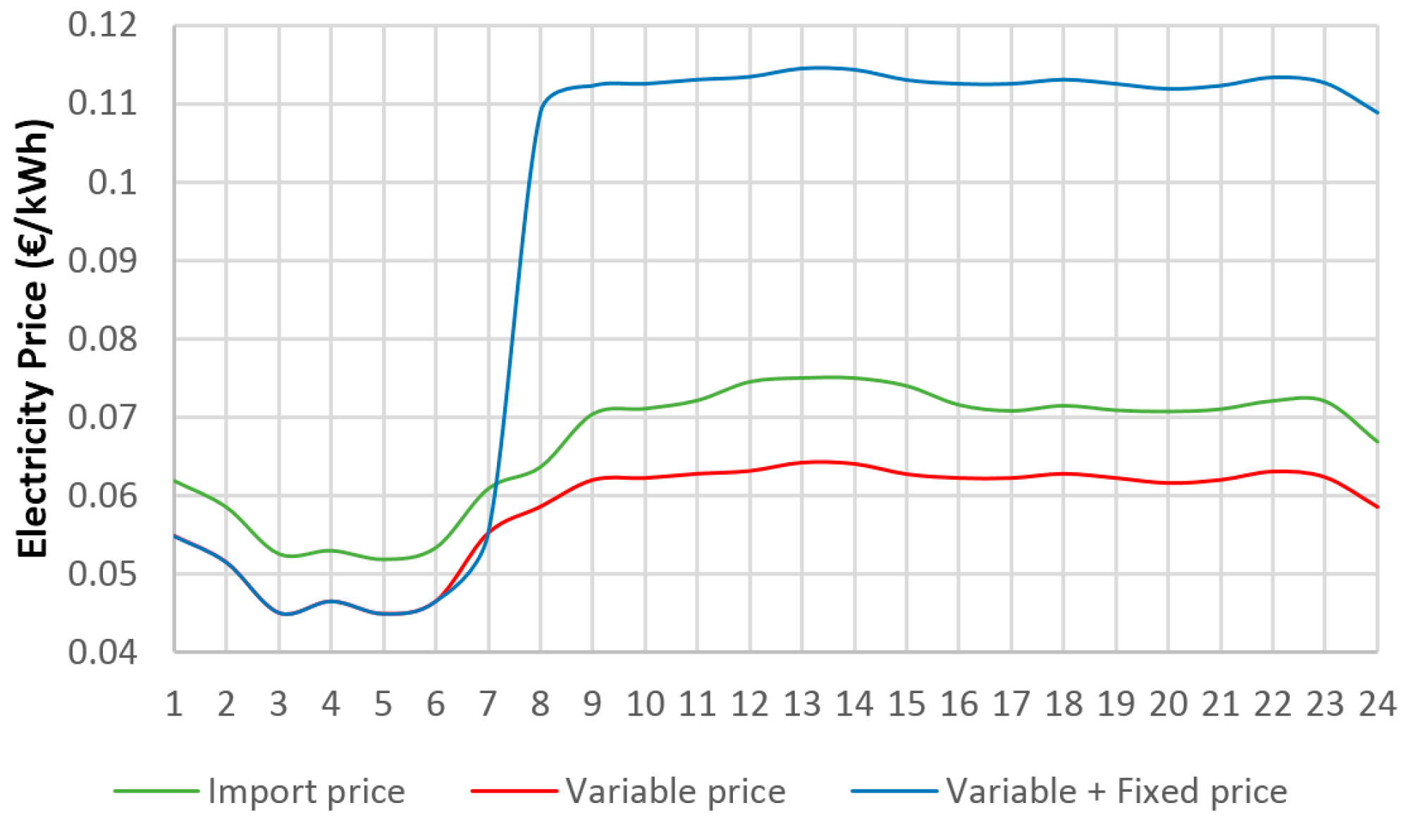
The days selected for the analysis include weekdays and weekend days. The required inputs are the hourly demand for each day and some parameters such as the price of electricity, heating and cooling sold to the DHC end users, nominal capacity of each unit, maintenance costs, etc. The considered cost of natural gas is 30.2 €/MWh. The price of the electricity fluctuates along the day and has two contributions, a fixed and a variable cost. Some restrictions are added to the model to avoid continuous on-off of the same unit. The partial load performance of each unit has been modelled using the plant operational data and the nominal performance provided by the manufacturer. The assumed maintenance costs for the cogeneration engines, thermal chillers, compression chiller, boiler and storage system are 20 €/h, 6 €/h, 15 €/h, 0.3 €/h and 15 €/h, respectively.
The trigeneration primary energy savings (PES) indicator (Equation (52)) is used to compare the different operational configurations. A crucial point in the numerical assessment of the primary energy saving is the merit of assigning suitable values to the reference efficiencies, which, in general, will depend on the technologies replaced. There are no official guidelines for this kind of reference efficiencies. In the following analysis intermediate efficiency values have been assumed, in particular: electrical efficiency was set equal to 0.45, thermal efficiency to 0.95 and the COP of the compression chiller equal to 5:
P E S ( j ) = 1 i = 1 3 I C E fuel ( i , j ) i = 1 3 I C E El 0.45 + H W to users 0.95 + Q eva S E + Q eva D E 0.45 × 5

4. Results

In this section the model has been applied to study the daily optimal operation in a representative day of summer and later the preferential selection for each type of absorption chiller according to different factors.

4.1. Daily Optimal Operation of the Plant

The developed model can be used to evaluate the daily optimal operational strategy and to analyse the differences with the real schedule of the plant. Of course, because of the simplicity of the model, it is not possible to take into account the transitional periods of the units, especially for the thermal chillers, but the optimizations can offer important information about the amount of working hours of each component and its capacity level. The model is used for evaluating alternative strategies to those adopted by the plant, in typical days. Each day is subdivided in 24 time steps. Then, with the aid of a spreadsheet created in Microsoft Excel, it was possible to evaluate the average daily performance parameters and the PES.
The day taken into account as an example here is a day of June when the plant works with all the internal combustion engines (ICEs) simultaneously at full capacity. The engines are switched ON at 8 h and switched OFF at 24 h, their transitional time is quite short, almost 20 min. The peak cooling demand is around 42% of the total capacity of both thermal chillers. The trends of the cooling demand and of the import and export electricity price are shown in Figure 4 and Figure 5.
The electricity price of the exported electricity has two terms, one of them follows the market price (red line in Figure 5) and changes continuously and the other is a fixed term. The blue line in Figure 5 represents the final price of the exported electricity and the green one the price for the electricity in the case that it was imported.
In the actual operational mode, the thermal chillers run during the same period as the engines. In the morning, they produce, more or less, a stable power, with the double effect that reaches an output of more than 3 MW, while in the afternoon there is a production decrease (Figure 6). The trend of the single effect and double effect absorption chillers is very similar. During the night the use of the compression chiller is necessary, with two peaks, at the beginning and at the end, and a constant production in the middle of the night.
Instead at the optimized solution (Figure 7), the DE chiller works during the same hours as the engine at the maximum limit imposed while the single effect works from 8 h to 12 h and from 17 h to 22 h. The total production of cooling in both cases is nearly the same, 16,000 kWh. Certainly, taking into account the transitional time of the machine (about 20 min), it could not be convenient stop it in the middle of the day from a practical point of view but the energy storage tank is better used in this case, as will be shown later.
Figure 8 and Figure 9 show how the demand is covered in both cases. In the actual schedule the storage is used only during the night, from 2 h to 8 h, with a peak of discharge power of almost 2000 kW while, in the suggested schedule of the optimization the storage is used during the night and also from 13 h to 16 h, when the single effect absorption chiller is switched OFF. This chiller contributed also to the charge of the storage. The maximum energy stored is about 15,000 kWh (Figure 10) and is completely empty when the engines restart.
The economic revenue with the optimized solution and the actual plant operation are compared in Table 4. The operation cost is higher with the proposed solution but the economic benefit is slightly higher because of a better use of the cooling storage system that saves electricity from the compressor unit at night.
The CO2 emissions increase with the number of hours that the engines are running. To obtain a reduction in emissions the engines have to be switched off for some hours. Thus the maximum economic benefit for a typical day coincides with the highest level of emissions. Trigeneration systems present higher efficiency than conventional energy supply systems and the possibility for sale of electricity to the electric grid is an important way to profit. However, this not necessarily represents reduction in emission, which depends on the local energy supply and on the source of electricity substituted.
As mentioned before the electricity price has two terms, one of them follows the market price and changes continuously and the other is a fixed term (Figure 5). As is shown in Figure 11 the trigeneration operation mode is only interesting after a fixed contribution of at least 2 c€/kWh. And for a value higher than 2.86 c€/kWh some engines can start to work all the day for the fixed natural gas cost. Obviously, the profitability of the plant depends also on the ratio between both the cost of the electricity and that of the natural gas. For this plant this ratio is 2.47. This means that for a cost ratio above this value the plant can operate in trigeneration mode producing economic benefits.

4.2. Optimal Sharing of the Cooling Load between Absorption Chillers

The typical cooling load demand selected as representative of the current plant operation is the one shown in the previous Figure 4. The peak load in this case is about the 40% of the total installed capacity of the absorption chillers.
In the previous analysis the data of the real plant is used to develop the model (type of units included, range and efficiency values, etc.) and to optimize the plant daily operation. Now, using this model some capacity limits have been applied to each chiller to analyze the effect of the distribution of the cooling demand among the different type of chillers. To distribute the load among both absorption chillers using the available waste heat, capacity limits have been imposed to the model to check the effect on the PES and the optimal load for each chiller. Figure 12 shows the daily PES for this plant using these limits. This value corresponds to the average PES for the analysed day (maximum cooling load demand equal to 40% of the total nominal capacity of the plant). The dashed lines represent configurations that are not acceptable since the use of the compression chiller is necessary to charge the storage during the night in order to cover the demand during the day; the solid lines therefore represent acceptable solutions. As shown in Figure 12, the best PES values are obtained when the capacity limits are set higher than 50% for both chillers. This means that the best efficiencies correspond to the case when both chillers work at high capacity but not too high to reduce the load of the other chiller excessively. The load sharing for all cases is presented in Figure 13. Each column represents the total production of both units, in particular the dark blue column is the portion produced by the single effect absorption chiller while the light blue color is the portion produced by the double effect absorption chiller. Solutions that require a massive use of the compressor are not taken into account. The best configurations are highlighted with the use of red line rectangles for the columns representing the production of the SE. The best allocation of the cooling load between both chillers has to be chosen between the configurations that produce the highest daily cooling production. Also it is convenient to choose the configurations were the contribution of the SE absorption chiller is relevant to get a high PES as shown in Figure 12. In this way the amount of hot water to dissipate generated by the engines is lower. According to these results the load of the SE chiller has to be selected between 70% and 80% and between 50% and 60% for the DE chiller.
The evolution of the objective function that corresponds to the plant economic revenue increases continuously with the increase in the limit capacity of the chillers as shown in Figure 14. Thus the highest value corresponds to the highest capacity limits. In this case the optimization procedure decides to work preferably with the more efficient chiller, the double effect chiller as seen in the right-side columns of Figure 13. However, to get a balanced plant operation and a similar PES it is more convenient to work with an important contribution of the SE chiller around 70% or higher.

5. Conclusions

The model developed was used to optimize the daily plant operation and to study the optimal cooling load sharing between the different types of chillers and a cooling storage system using the primary energy saving indicator as the main parameter to compare the different load distribution configurations for a given cooling demand. This distribution is heavily influenced by the price of the electricity sold to the grid which rules the duration of the operation time of the engines. The load sharing strategy was studied for a typical day. Cooling load distribution among the different chillers changes with the cooling load of the whole trigeneration plant because of the characteristic part-load chiller performance. The efficiency of the single effect chiller is the lowest one but its operation is important to increase the heat recovery of the cogeneration engines and reduce the cost of engines cooling heat rejection. The actual COP of the single- and DE chillers is reasonably acceptable in spite of the low cooling load of the plant, between 0.6–0.65 and close to 1, respectively for a load around 40% of its nominal capacity.
From the economic point of view the operational optimization approach prefers to use the double effect chiller as much as possible because it is more efficient but to get an acceptable saving in primary energy it is interesting to work also with the single effect chiller at around 70%–80% of its maximum capacity to avoid excessive dissipation of heat to the ambient and obtain good primary energy savings. In the future it could be interesting to compare the present configuration using separately the exhaust gas waste heat in a double effect and the engine cooling in a single effect, with another configuration using both sources of waste heat in the same double effect chiller, using the exhaust gas at the high pressure generator and the lower temperature waste heat at the low pressure generator. It is not clear which is the most efficient but probably the one used in this paper will be more flexible from the operation point of view. The presented model is very useful to study plant operation strategies and allocate the different cooling loads among the different chiller types and the storage system.

Acknowledgments

The authors acknowledge the collaboration of the company Poligeneració Parc de l’Alba ST4 S.A. in this study and the financial support of the Spanish Ministry of Economy and Competitiveness and FEDER (Proj. DPI2012-38841-C02-01).

Author Contributions

Benedetto Conte performed the modelling, optimization and analysis of results under the guidance of Joan Carles Bruno. The paper was written by Joan Carles Bruno with the support of Benedetto Conte and revised by Alberto Coronas.

Conflicts of Interest

The authors declare no conflict of interest. The founding sponsors had no role in the design of the study; in the collection, analyses, or interpretation of data; in the writing of the manuscript, and in the decision to publish the results.

References

  1. Rezaie, B.; Rosen, M.A. District heating and cooling: Review of technology and potential enhancements. Appl. Energy 2012, 93, 2–10. [Google Scholar] [CrossRef]
  2. Ortiga, J.; Bruno, J.C.; Coronas, A. Operational optimisation of a complex trigeneration system connected to a district heating and cooling network. Appl. Therm. Eng. 2013, 50, 1536–1542. [Google Scholar] [CrossRef]
  3. Canelli, M.; Entchev, E.; Sasso, M.; Yang, L.; Ghorab, M. Dynamic simulations of hybrid energy systems in load sharing application. Appl. Therm. Eng. 2015, 78, 315–325. [Google Scholar] [CrossRef]
  4. Entchev, E.; Yang, L.; Ghorab, M.; Lee, E.J. Simulation of hybrid renewable microgeneration systems in load sharing applications. Energy 2013, 50, 252–261. [Google Scholar] [CrossRef]
  5. Piacentino, A.; Barbaro, C. A comprehensive tool for efficient design and operation of polygeneration-based energy μgrids serving a cluster of buildings. Part II: Analysis of the applicative potential. Appl. Energy 2013, 111, 1222–1238. [Google Scholar] [CrossRef]
  6. Abou-Ziyan, H.Z.; Alajmi, A.F. Effect of load-sharing operation strategy on the aggregate performance of existed multiple-chiller systems. Appl. Energy 2014, 135, 329–338. [Google Scholar] [CrossRef]
  7. Sun, Y.; Wang, S.; Huang, G. Chiller sequencing control with enhanced robustness for energy efficient operation. Energy Build. 2009, 41, 1246–1255. [Google Scholar] [CrossRef]
  8. Yu, F.W.; Chan, K.T. Optimum load sharing strategy for multiple-chiller systems serving air-conditioned buildings. Build. Environ. 2007, 42, 1581–1593. [Google Scholar] [CrossRef]
  9. Underwood, C.; Ng, B.; Yik, F. Scheduling of multiple chillers in trigeneration plants. Energies 2015, 8, 11095–11119. [Google Scholar] [CrossRef]
  10. Hajabdollahi, H.; Ganjehkaviri, A.; Jaafar, M.N.M. Assessment of new operational strategy in optimization of CCHP plant for different climates using evolutionary algorithms. Appl. Therm. Eng. 2015, 75, 468–480. [Google Scholar] [CrossRef]
  11. Chicco, G.; Mancarella, P. Matrix modelling of small-scale trigeneration systems and application to operational optimization. Energy 2009, 34, 261–273. [Google Scholar] [CrossRef]
  12. Stojiljkovic, M.M.; Blagojevic, B.D. Multi-Objective Combinatorial Optimization of Trigeneration Plants Based on Metaheuristics. Energies 2014, 7, 8554–8581. [Google Scholar] [CrossRef]
  13. Cho, H.; Smith, A.D.; Mago, P. Combined cooling, heating and power: A review of performance improvement and optimization. Appl. Energy 2014, 136, 168–185. [Google Scholar] [CrossRef]
  14. Roque Díaz, P.; Benito, Y.R.; Parise, J.A.R. Thermoeconomic assessment of a multi-engine, multi-heat-pump CCHP (combined cooling, heating and power generation) system—A case study. Energy 2010, 35, 3540–3550. [Google Scholar] [CrossRef]
  15. Carvalho, M.; Serra, L.M.; Lozano, M.A. Optimal synthesis of trigeneration systems subject to environmental constraints. Energy 2011, 36, 3779–3790. [Google Scholar] [CrossRef]
  16. Rodriguez-Aumente, P.A.; Rodriguez-Hidalgo, M.C.; Nogueira, J.I.; Lecuona, A.; Venegas, M.C. District heating and cooling for business buildings in Madrid. Appl. Therm. Eng. 2013, 50, 1496–1503. [Google Scholar] [CrossRef]
  17. Jing, Z.X.; Jiang, X.S.; Wu, Q.H.; Tang, W.H.; Hua, B. Modelling and optimal operation of a small-scale integrated energy based district heating and cooling system. Energy 2014, 73, 399–415. [Google Scholar] [CrossRef]
  18. Buoro, D.; Casisi, M.; Pinamonti, P.; Reini, M. Optimal synthesis and operation of advanced energy supply systems for standard and domotic home. Energy Convers. Manag. 2012, 60, 96–105. [Google Scholar] [CrossRef]
  19. Park, C.W.; Jeong, J.H.; Kang, Y.T. Energy consumption characteristics of an absorption chiller during the partial load operation. Energy 2004, 73, 399–415. [Google Scholar] [CrossRef]
  20. Le Lostec, B.; Galanis, N.; Millette, J. Experimental study of an ammonia-water absorption chiller. Int. J. Refrig. 2012, 35, 2275–2286. [Google Scholar] [CrossRef]
  21. Martínez-Maradiaga, D.; Bruno, J.C.; Coronas, A. Steady-State data reconciliation for absorption refrigeration systems. Appl. Therm. Eng. 2013, 51, 1170–1180. [Google Scholar] [CrossRef]
  22. Yokoyama, R.; Shinano, Y.; Taniguchi, S.; Ohkura, M.; Wakui, T. Optimization of energy supply systems by MILP branch and bound method in consideration of hierarchical relationship between design and operation. Energy Convers. Manag. 2015, 92, 92–104. [Google Scholar] [CrossRef]
  23. Voll, P.; Klaffke, C.; Hennen, M.; Bardow, A. Automated superstructure-based synthesis and optimization of distributed energy supply systems. Energy 2013, 50, 374–388. [Google Scholar] [CrossRef]
  24. Polycity: Energy Networks in Sustainable Cities; Eicker, U. (Ed.) Kraemer Verlag: Stuttgart, Germany, 2012.
  25. Keil, C.; Plura, S.; Radspieler, M.; Schweigler, C. Application of customized absorption heat pumps for utilization of low-grade heat sources. Appl. Therm. Eng. 2008, 28, 2070–2076. [Google Scholar] [CrossRef]
  26. Ziegler, F. Adaptation of modular absorption chillers in order to optimize performance in district heating networks, Keynote speech. In Proceedings of the 3rd International Conference on Polygeneration, Anna University, Chennai, India, 18–20 February 2015.
Figure 1. Configuration of the trigeneration plant (ST4) and main energy streams.
Energies 09 00573 g001
Figure 2. COP of the SE absorption chiller as a function of the load.
Energies 09 00573 g002
Figure 3. COP of the DE absorption chiller as a function of the load.
Energies 09 00573 g003
Figure 4. Chilled water demand in kWh.
Energies 09 00573 g004
Figure 5. Electricity price in €/kWh.
Energies 09 00573 g005
Figure 6. Actual chilled water production (kWh).
Energies 09 00573 g006
Figure 7. Optimized chiller water production (kWh).
Energies 09 00573 g007
Figure 8. Actual coverage of the demand (kWh).
Energies 09 00573 g008
Figure 9. Optimised coverage of the demand (kWh).
Energies 09 00573 g009
Figure 10. Hourly energy level of the storage (kWh).
Energies 09 00573 g010
Figure 11. Objective Function (€/day) for different electricity fixed term (€/kWh).
Energies 09 00573 g011
Figure 12. Daily primary energy savings (PES) (%) for different maximum capacities for each chiller.
Energies 09 00573 g012
Figure 13. Sharing of the load (kWh) between the single and DE chiller.
Energies 09 00573 g013
Figure 14. Objective function as a function of the capacity limits for each chiller.
Energies 09 00573 g014
Table 1. Nominal conditions (NC) and actual working conditions of the single-effect (SE) absorption chiller for different steady-state periods of certain days. COP: coefficient of performance; Temp.: Temperature.
TagUnitNC29.0512.0623.0708.0916.1128.1108.0330.06
Temp. Hot Water in SE°C94.087.587.686.986.691.890.189.490.7
Temp. Hot Water out SE°C78.053.659.660.364.949.256.943.546.4
Flow Hot Waterm3/h234.037.061.355.382.618.942.416.618.9
Heat transfer Gen.kW43661459199417092083933.11635883.5972.7
Temp. Ch Water out°C6.55.05.04.96.15.05.55.05.0
Temp. Ch Water in°C13.06.47.26.98.05.97.35.95.8
Flow Ch Waterm3/h433.0470.3467.4408.0467.4392.1439.1397.9453.3
Heat transfer Evap.kW3275790.51159919.21041427.6899.5412.2448.8
COP 0.750.540.580.540.500.460.550.470.46
Temp. CW in°C30.026.028.928.330.627.727.925.626.1
Temp. CW out°C37.028.131.930.733.428.730.026.127.2
Flow CWm3/h940.0868.7862.7882.8885.2896.2884.1850.7878.4
Heat rejected CWkW7641206530572441292011092105552.41144
Heat losseskW0.0184.596.0187.2204.0251.7429.5743.3277.5
Table 2. NC and actual working conditions of the double-effect (DE) absorption chiller for different steady-state periods of certain days. ICEs: internal combustion engines.
TagUnitNC29.0512.0623.0708.0916.1128.1108.0330.06
Temp. ExGas all°C398.0379.8382.1383.1386.1387.9373.9392.9378.1
Temp. ExGas out DE°C170.0142.0166.6158.2163.0112.3137.3134.0136.5
Flow Exh Gaskg/h540,00038,95041,77632,04536,41816,72832,28523,24330,870
Heat ExGas All ICEskW387029342851220224831408233518392278
Temp. Ch Water out°C6.54.54.54.45.85.25.05.24.5
Temp. Ch Water in°C13.07.48.27.99.16.98.27.76.8
Flow Ch Waterm3/h661.0704.5699.1609.0699.5582.7654.4659.4677.8
Heat transfer Evap.kW502823633025250126351149241418831807
COP 1.300.801.061.141.060.821.031.020.79
Temp. CW in°C30.024.126.826.228.526.026.124.624.1
Temp. CW out°C37.027.931.930.432.927.729.727.727.3
Flow CWm3/h1080.01017.31010.31034.31035.0928.01033.51017.91028.9
Heat rejected CWkW889844895995505553791854431337103907
Heat losseskW0.0808.0119.0352.0261.0703.0436.012.0178.0
Table 3. Estimated power for each pump of the system. CC: compression chiller.
EquipmentCircuitPower (kW)
EnginesLow temperature circuit7.8
High temperature circuit22.8
Cooling tower12.6
SEHot water circuit22
Chilled water38
Condenser/absorber circuit98
DEChilled water circuit60
Condenser/absorber circuit118
CCChilled water circuit50
Condenser/absorber circuit69
Table 4. Comparison of the optimised and actual operation of the plant in a typical day of June.
CostModelActual
Maintenance costs (€)12921253
Operational costs (€)11,24610,938
Income (€)19,82519,410
Economic revenue (€)72877219

