1. Introduction
With the progressively prominent energy shortage and the deteriorating climate, the significance of renewable energy has reached new heights. Photovoltaic (PV) power generation, which is the renewable energy that is most suitable for developing universally due to its convenient installation and the illimitation of territorial factors, has drawn significant attention. Based on the relevant statistics, the newly installed capacity of PV power in China in 2015 was 15.13 MW, which was over a quarter of the global newly installed capacity. By the end of 2015, the accumulated installed capacity had reached 43.18 MW, and China attained the maximum PV capacity in the world. Furthermore, the PV market scale of China will keep expanding, and the preliminary target scale of PV installed capacity will reach approximately 150 MW in five years. Under the support of Chinese national policy, the Chinese PV industry has developed rapidly in recent years. Nevertheless, the randomness and intermittence of PV output are sensitive to variables such as climate factors and geology environments. These uncertainties in the PV output have inevitably aggravated the difficulties in power system dispatching, becoming one of the most significant obstacle for power grid to consume PV power. Furthermore, the high permeability of PV power production might not be beneficial to the economical, safe and reliable operation of the power grid. Due to the limited ability to consume PV power of power system, there appears to be a serious phenomenon of abandoning PV power in China. According to the statistical data of the National Energy Administration of China, the phenomenon of abandoning PV power in northwestern China is intensely severe, where the abandonment rates in Gansu Province and in Xinjiang Province were 31% and 26% in 2015, respectively, corresponding to an abandoned capacity of 1.897 MW and 1.0556 MW, respectively. Therefore, the precise forecast of PV power plays a vital role in reducing the impacts of uncertainties of PV output, achieving a reasonable power dispatch, decreasing power generation costs, raising the utilization rate of PV units, promoting the development of PV enterprises and finally obtaining higher general social benefits [
1,
2,
3,
4,
5,
6,
7].
Used for different prediction targets, the direct forecast and the indirect forecast are the two major methods for PV output forecasting. The direct forecast is used to predict the PV output in a straightforward manor, whereas the indirect forecast relies on the prediction of radiation intensity. The two major realization approaches for PV power forecast modeling are the statistical method and the physical method. Depending on the accuracy of the mathematical model for the photoelectric conversion process, the calculation of the physical method can be complex. The universally employed statistical methods include Markov chains, neural networks, autoregressive and moving average models, and support vector machines [
8,
9].
In the studies relevant to PV power forecasts, the influence of the climate variables has been investigated thoroughly. Zhu et al. [
10] provided a distance analysis measure to analyze the correlations between the weather variables and the PV output and used SOM clustering to identify different sample types to develop a PV forecast model rooted in climate clustering recognition. Dai et al. [
11] combined numerical weather prediction with ground-based cloud images and analyzed the effect of the power attenuation caused by the cloud cover of an electric station on the forecasted PV output. In [
12], a weather-based hybrid method for a one-day ahead hourly PV power forecast is presented to improve the real-time control performance and reduce the possible negative impacts on PV systems.
The investigations above consider the influence of the climate to improve the accuracy of the forecast; nevertheless, forecast error is inevitable. Gao et al. [
13] constructed a probabilistic model for the photovoltaic forecast, and simulated the random errors caused by the prediction. Zhao et al. [
14] presented a probabilistic density simulation of the PV power conditional prediction error on the foundation of Copula theory. However, establishing the model of the forecast error is unable to satisfy the need to elevate the forecast accuracy. To further increase the forecast accuracy of the PV power, error calibration is introduced in this paper. Liu et al. [
15] applied error calibration to Chinese medium- and long-term power load forecasting by establishing a forecast model that combined general autoregressive conditional heteroscedasticity with regression. Song et al. [
16] proposed a new error correcting approach for load forecasting in power systems by using trajectory tracking stability theory. To improve the accuracy of wind speed forecasting, a method based on a relevant vector machine and an auto-regressive moving average error correcting is proposed in [
17]. Liu et al. [
18] adopted a hidden Markov model to analyze the forecast error due to the price of electricity and the error distribution of the model in different states. In general, in the fields of load forecast, wind speed forecast, and electricity price forecast, error calibration could contribute to a reduction to the prediction error. Consequently, error calibration is introduced into PV power forecasting here to improve the prediction accuracy.
Due to the effect of meteorological factors on PV power, a short-term PV power forecast model based on error calibration under typical climate categories is developed, applied to the day-head PV power forecast. In the proposed model, the typical climate categories are defined, and according to which, the historical PV power data are divided. On this basis, the probability density function (PDF) curve of forecast data for each category is simulated using a mathematical distribution, and samplings are performed to achieve the sampling values of the error. In addition, sequencing the sampling values by the compensation values of the error from the fluctuation analysis, the fitted values of the error can be obtained. Finally, the superposition of the forecasted PV power values and the fitted values of the error is conducted to improve the forecast accuracy.
2. Research Route of a Short-Term PV Power Forecast Based on Error Calibration
There exist two types of error calibration methods to date. One is to apply a statistical approach to simulating the PDF curves of the PV power forecast error by judging the probability density features of which the error of the next time point would be analyzed and estimated. The other is to predict the error value of the next time point directly using mathematical models to correct the PV power forecast values with the predictive values of the error.
In the application of the first method, it is universally assumed that the forecast error of PV power obeys a normal distribution [
19,
20]. Nevertheless, simulations using normal distribution tend not to be of very high accuracy in the majority of the cases, and therefore, they are unable to describe the error distribution of the PV power forecast precisely. Furthermore, it would be difficult for the unordered simulated values of the error acquired by a statistical approach to correspond to the PV forecast power. The second method for error prediction mainly relies on the mathematical model chosen and analyzing future error based on the data characteristics of the historical error. However, the forecasting accuracy might be limited, especially in the case of strong error volatility.
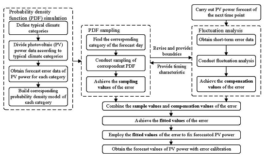
Focusing on the two error forecasting approaches mentioned above, a two-step method that employs a statistical approach to build the probabilistic model of the short-term PV power forecast error and then adopts a fluctuation analysis to process the statistical results. The specific steps are as follows:
- (1)
The typical climate categories are defined to classify the historical data of the PV power.
- (2)
Due to the noticeably different amplitude features of the forecast error of PV power, the probability density distributions of forecast error are generated for each category.
- (3)
Perform parameter fitting on the PDF curves for each category to establish the corresponding fitted PDF model to gain the sampling values of the error.
- (4)
Determine the predictive approaches and compensation methods by analyzing the fluctuation characteristics of the forecast error, and then predict the error of the next time point to gain the compensation values of the error.
- (5)
Employ the sequential compensation values obtained by the fluctuation analysis to sequence the sampling values of the error. The sampling values that are closest to the compensation ones are chosen to be the fitted values of the error at the corresponding time points.
- (6)
Utilize the fitted values of the error to correct the PV power forecast.
The advantages of this proposed method are as follows:
- (1)
Provides sampling values of the error with a timing characteristic by fluctuation analysis to fit the unordered sampling results to the PV power forecast values.
- (2)
Utilize a probabilistic model of the historical forecasting error to modify the fluctuation analysis results of the recent error and provide boundaries for them, which could avoid a divergence of error and overcompensation.
The basic structure of the method proposed is shown in
Figure 1.
3. Sampling Values Generation of the PV Power Forecast Error under Typical Climate Categories
3.1. Classification of Typical Climate Categories
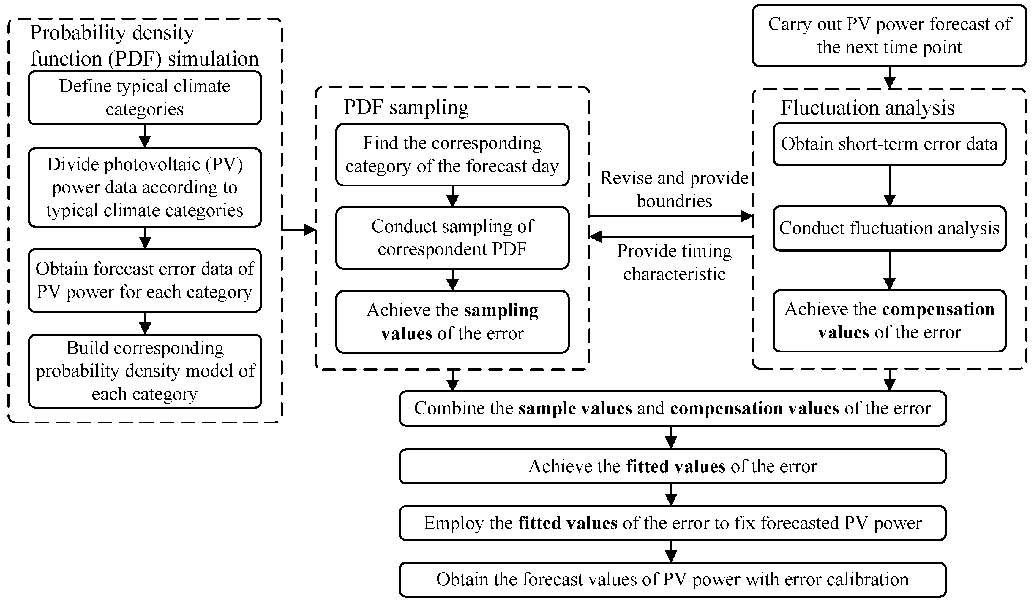
PV power is closely related to climate conditions, which depend on a range of issues and can be described by many different approaches. To define the classification of climate categories using a harmonized standard, the China Meteorological Administration released “GB/T 22164—2008 Public Climate Service—Weather Graphic Symbols”, on which 33 types of climate categories are defined [
21]. On that basis, the weather conditions can be classified into four categories that represent the most vital characteristics of these climates, which include Sunny, Cloudy, Drizzle and Heavy rain [
8]. However, the range of PV power for each category varies over the different seasons. For instance, the maximum PV output on sunny days in summer is apparently higher than it is in winter. Consequently, the classification of the typical climate categories is based on both the weather and the season, which generates a total of 16 categories, as shown in
Figure 2.
3.2. Distribution of the PV Power Forecast Error under Typical Climate Categories
In this paper, the relative error (RE) of the PV power forecast is employed to describe the forecast accuracy, and the definition of which is shown in Equation (1).
where δ
i is the RE of the
i-th forecasting node; and
Pf,i and
Pa,i are the forecast value and actual value of the
i-th forecasting node, respectively.
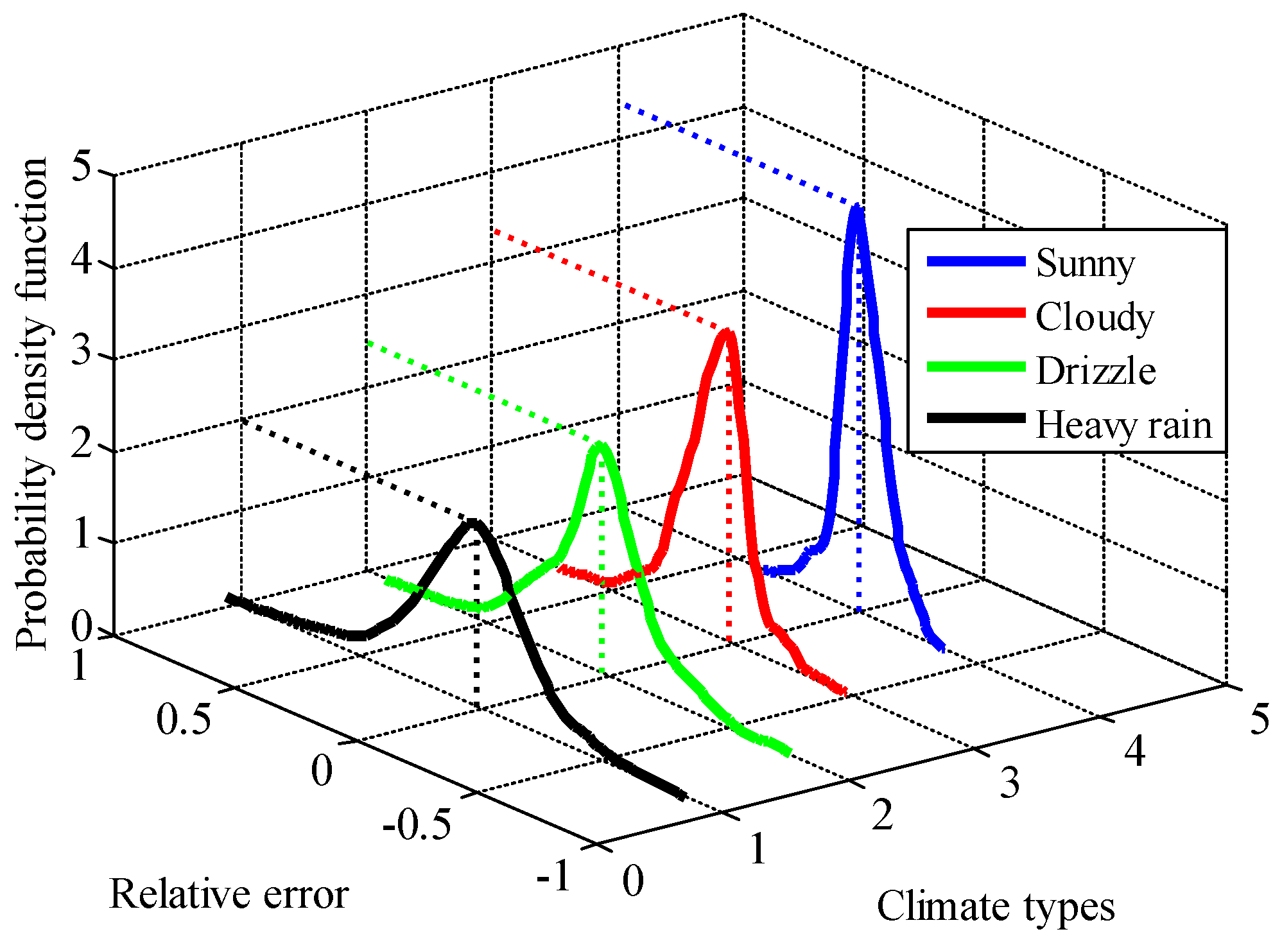
The probability density function (PDF) of the RE predicted by the wavelet neural network (WNN) [
22] of the Polycrystalline Silicon Photovoltaic Array (10 kW) in the State Key Laboratory of New Energy Power System at the North China Electric Power University (Baoding, China) in spring is shown in
Figure 3. Regardless of the climate type, the PDF of the RE is unimodal and almost symmetric, and the peak time is when the RE value is approximately zero. Moreover, the values of the PDF tend to decline with an increase in the RE absolute values and ultimately reach zero.
The variances of the PDFs corresponding to the four climate types are expressed as , , and . The RE values in sunny weather are the most concentrated, that is when the minimum variance of the four curves is achieved, and illustrates a “tall and thin” characteristic. In comparison, when it rains heavily, the PDF curve would appear to be “short and fat”, which indicates a smaller variance . Universally, the variances of the RE have tendency to be larger when the weather types vary from sunny to cloudy to drizzle to heavy rain, successively, and therefore, < < < . This relationship between the variances exists in every season.
Based on the analysis above, distributions of the RE of the PV power forecast can be concluded to be approximately regular probability density distributions for each typical climate category. Consequently, an appropriate unimodal PDF would be adopted to simulate the distribution of the RE for each typical climate category.
3.3. The PDF Generation of the PV Power Forecast Error Based on a Nonparametric Kernel Density Estimation
3.3.1. Basic Theory of Nonparametric Kernel Density Estimation
Based on data sample completely, nonparametric kernel density estimation (NKDE) is a method to study the data distribution with no prior knowledge. The application of NKDE is universal in multiple fields, such as load modeling, wind speed modeling, and reliable index calculation [
23]. To simulate the RE of the PV power forecast, an NKDE is employed to fit the parameters of the PDF based on the typical climate categories.
The PDF fk(δ) of the RE δ can be obtained using Equation (2).
where
h is the bandwidth;
n is the sample number; δ
i is the
i-th sample of the PV power; and
K is the kernel function.
In order to guarantee the continuity of the PDFs, the kernel functions are usually smoothed unimodal PDFs, which satisfy the conditions in Equation (3).
where
c is a positive constant.
The most commonly used kernel functions are the Epanechikov function and Gaussian function. In this paper, the Gaussian function, which is shown in Equation (4), is adopted.
3.3.2. Selection of the Optimal Bandwidth
The bandwidth
h affects the accuracy of the NKDE greatly. According to the kernel density estimation theory [
24,
25], the probability density would be over scattered and the curve of
fk(δ) would be over smooth if
h is too large, which may neglect certain crucial structural features of the distribution. Otherwise, if
h is too small, the density estimation tends to concentrate around the data given, and the wrong peak values would appear on the
fk(δ) curve, which may then lack smoothness and become overfitted.
The definition of the asymptotic mean integrated square error (AMISE) is shown in Equation (5).
where σ
k is the standard deviation of the kernel density function; and
f is the actual probability density distribution of the sample. When
n→∞,
h→0 and
nh→∞, then
AMISE(
h)→0. By minimizing the AMISE, the optimal bandwidth
hopt is obtained, as shown as Equation (6).
Therefore, the optimal bandwidth relies on the probability density
f, which is unknown. According to the rule of thumb [
26],
f could be replaced by the standard normal density function with a standard deviation of σ
k, as shown in Equation (7).
where σ is the standard deviation of the sample.
Generally, the standard deviation σ of the sample could be expressed by a divergence variable named the interquartile range (
IQR) that is a more robust measure. The optimal bandwidth can be expressed using Equation (8).
where Φ is a standard normal cumulative distribution function.
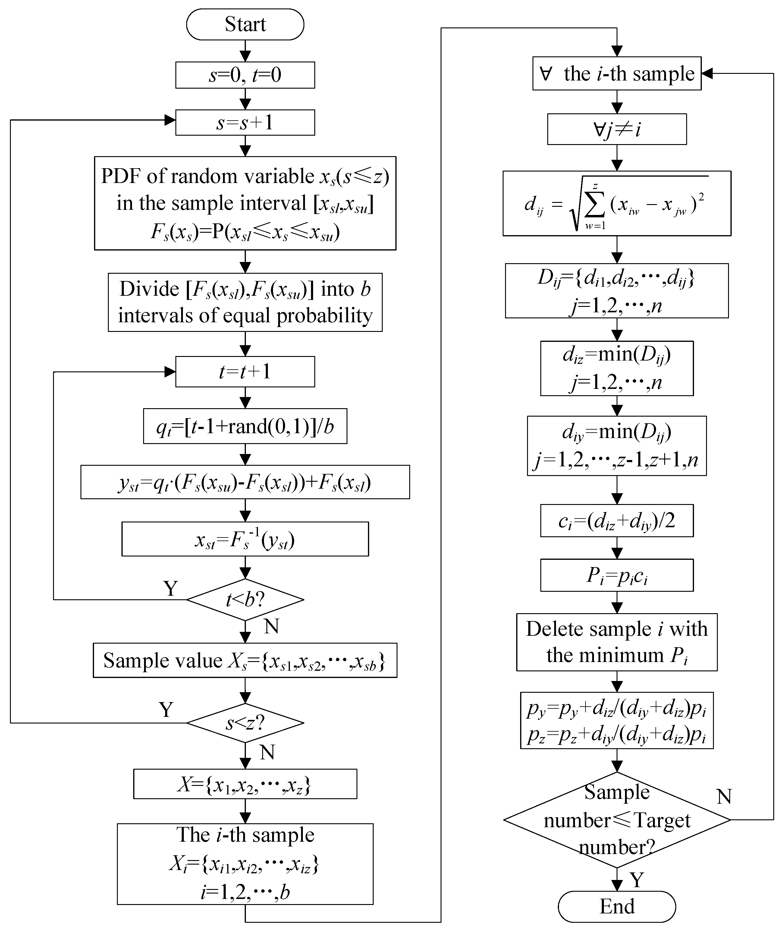
3.4. Sampling of the PV Power Forecast Error Based on Latin Hypercube Sampling and a Multi-Scenario Technique
Latin hypercube sampling is a multi-dimensional stratified sampling method, which is able to effectively restore the random effect. Latin hypercube sampling is combined with a multi-scenario technique [
27,
28] to perform the sampling of the fitted PDF of the RE in the classified categories. During sampling, the sampling size is assumed to be
b, and the random variable number is assumed to be
z. The variables can be represented as
X = {
x1,
x2,…,
xz}. After the sampling, the random variable number is reduced to
N. The specific steps of the Latin hypercube sampling and the scenario reduction are illustrated in
Figure 4.
4. Compensation Values Generation of the PV Power Forecast Error Based on Fluctuation Analysis
The uncertainties of PV power and the prediction methodologies are the main sources of PV forecast error. Considering the regularity of the fluctuated direction of the RE in short-term predictions, the fluctuation analysis of the RE is a feasible scheme to prejudge the tendency of the RE and to produce the corresponding compensation values of the RE [
29].
During the fluctuation analysis, n samples from the historical RE data are applied to develop the measuring standards for the short-term estimation. The long-term variance is presented as , and the critical value of the absolute slope of the straight-line fitting is presented as kl, as follows:
where
k1 and
k2 are the up and down critical values of the one-sided probability interval determined by the simulated model and the probability level, respectively.
Three RE values before the forecast time are chosen to be the short-term RE samples, and the calculation of the variance
and the absolute slope
ks of the straight-line fitting are performed. The calculation results of these two variables indicate the investigation methods for the RE fluctuation, as shown in
Table 1.
On the basis of the estimated values of the RE from the investigation methods in
Table 1, the error compensation rule is formed. The threshold δ
0 is the boundary value that separates large errors from small errors. By comparing the RE estimated values δ
i at the point
i and δ
i-1 at point
i − 1 to δ
0, the compensation methods of estimated RE would be ascertained, as in
Table 2.
Based on fluctuation analysis, the sampling results are sequenced using the compensation values. The sampling values closest to the compensation ones are elected to be the fitted values of the RE at the corresponding time points to correct the forecast values of the PV power, and moreover, to improve the forecast accuracy.
5. Short-Term PV Power Forecast Model Based on Error Calibration under Typical Climate Categories
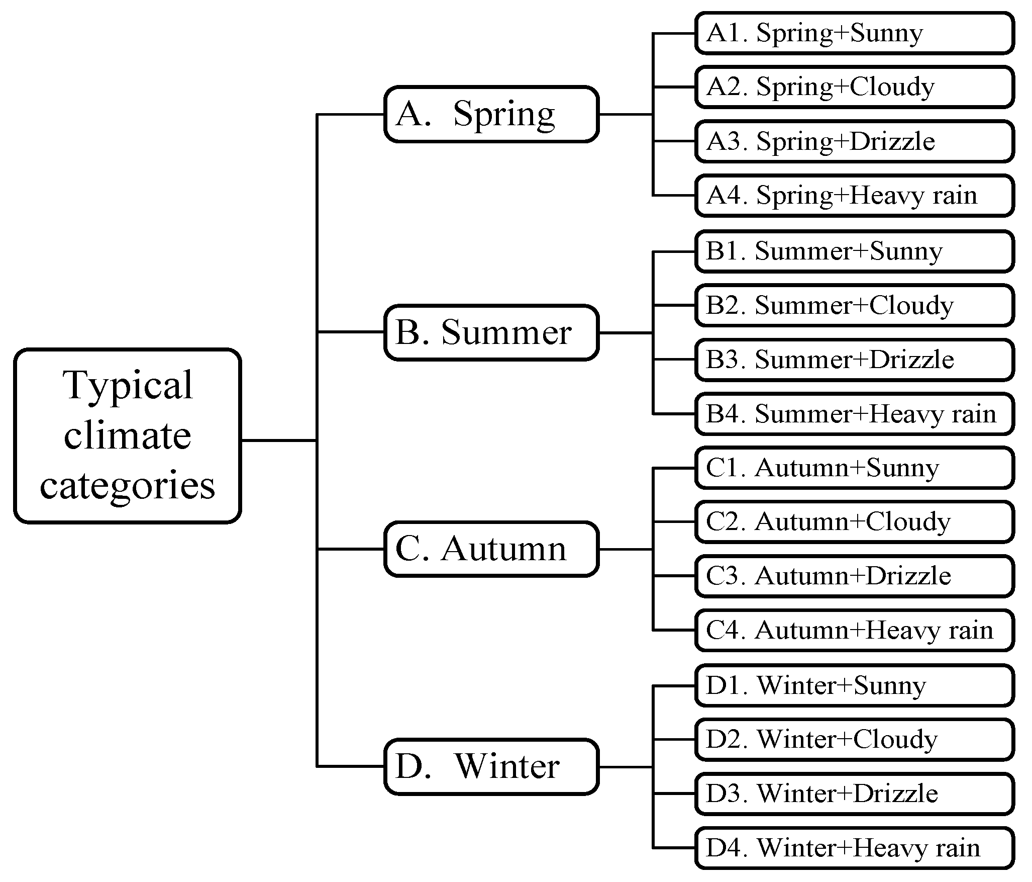
The concept of error calibration is applied to short-term PV power forecasts. By generating the fitted value of the forecast error and overlaying it on the forecasted values of the PV power, PV power forecast values with error calibration can be achieved. The basic concept of error calibration is shown in
Figure 5.
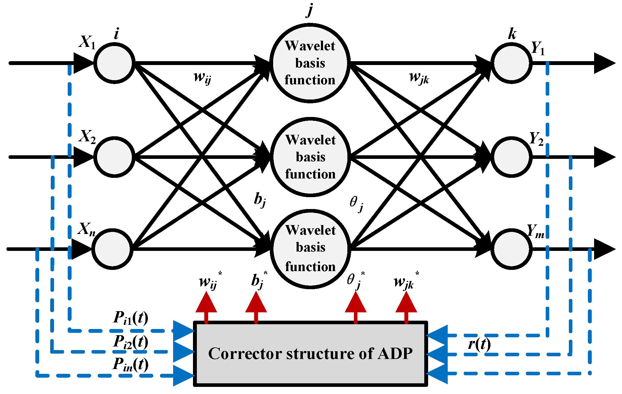
The WNN with adaptive dynamic programming (ADP) is applied to forecast the PV power [
30]. In the forecasting model, the wavelet function is employed to be the incentive function of the hidden layer in neural network, and the uniform approximation of the wavelet decomposition is conducted to combine the wavelet analysis and the neural network to achieve the output signal sequences. In addition, the concept of the predictor-corrector is introduced, according to which the actual measurement data are utilized to update the parameters of the WNN to improve the forecast accuracy. The basic theory is illustrated in
Figure 6.
In
Figure 6,
X1,
X2,…,
Xn are the inputs of the prediction model;
Y1,
Y2,…,
Ym are the outputs of the prediction model;
wij is the weight between the input layer and the hidden layer of the WNN;
wjk is the weight between the hidden layer and the output layer of the WNN;
bj is the expansion factor of the wavelet basis function; θ
j is the threshold;
Pi1(
t),
Pi2(
t),…,
Pin(
t) are the actual measurement data of the sampling period;
wij*,
wjk*,
bj*, θ
j* are the updated parameters after occupying the ADP corrector; and
r(
t) is the cost function.
The steps of the forecast model for a short-term PV power forecast based on error calibration under typical climate categories are demonstrated as follows:
- (1)
Define 16 typical climate categories according to the weather conditions and the seasons.
- (2)
Classify the historical PV power data into the typical climate categories and generate the probability density distributions of the RE for each category.
- (3)
Take advantage of an NKDE to develop a probabilistic model for the RE of the PV power forecast in each category and employ the optimal bandwidth to refine the fitted results.
- (4)
Conduct the PV power forecast by WNN with ADP on the next forecast day and determine which typical climate category the forecast day belongs.
- (5)
Employ a Latin hypercube sampling combined with a multi-scenario technique to perform a sampling of the fitted PDF curves of the RE in the corresponding typical climate category of the forecast day to obtain the sampling values of the RE.
- (6)
Perform a fluctuation analysis to calculate the compensation values of the RE for the next time point.
- (7)
Develop the measuring standards with the historical RE and sequence the sampling values according to the compensation values to obtain the fitted RE values of the PV power forecast for each time point.
- (8)
Combine the forecast values of the PV power in Step (4) with the fitted values of the RE in Step (7) to achieve PV power forecast values with error calibration.
6. Case Study
In this section, the method proposed has been tested using the normalized PV output data from Hebei Province, China in 2013 in a MATLAB simulation.
After the identification and processing of bad data as well as data normalization, the historical PV power data has been classified into 16 typical climate categories. The historical error data are provided by the WNN with ADP and the PDF curves of the RE in each category have been generated.
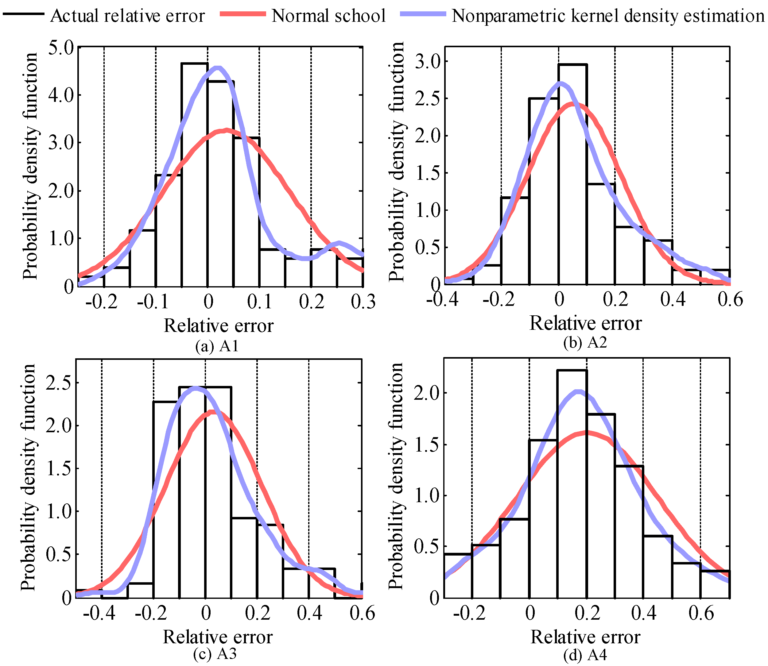
In comparison with a normal distribution, the simulation results of the fitted PDF curves of the RE in the spring by an NKDE are shown in
Figure 7. The results indicate that the normal distribution fitting has a larger discrepancy in comparison with those from the NKDE, which corresponded closely with the fluctuations in the original sample data. The simulation errors are measured by Mean absolute error (
MAE) and root mean square error (
RMSE), which are dimensionless because of the normalization of the PV output data. As shown in
Table 3, the simulation using the NKDE has an excellent fitting in contrast with the one using the normal distribution because the fitting error of the NKDE was two or three orders of magnitude less than that of the normal distribution.
In accordance with the theory mentioned above, the smoothness of the fitted curves would increase if the bandwidth of the NKDE increased; otherwise, peak values are more likely to appear. Concerning the PDF curves, the bounding areas with their abscissa are identical to 1. Accordingly, for the unimodal fitted PDF curves, larger bandwidths resulted in more concentrated distributions and smaller variances; correspondingly, when the bandwidths decreased, the distributions tend to be more divergent, which suggests larger variances of the PDF curves. The variances of the fitted PDF curves from A1 to A4 are 0.0346, 0.0593, 0.0692 and 0.0738, respectively, which is consistent with the characteristics of the RE, namely that < < < .
After finding the typical climate category that matches the forecast day, a PV power forecast is employed using a WNN with ADP. Mean absolute percent error (
MAPE),
MAE and
RMSE are employed to measure the forecast errors. The forecast accuracies by the WNN with ADP of the categories from A1 to A4 are shown in
Table 4.
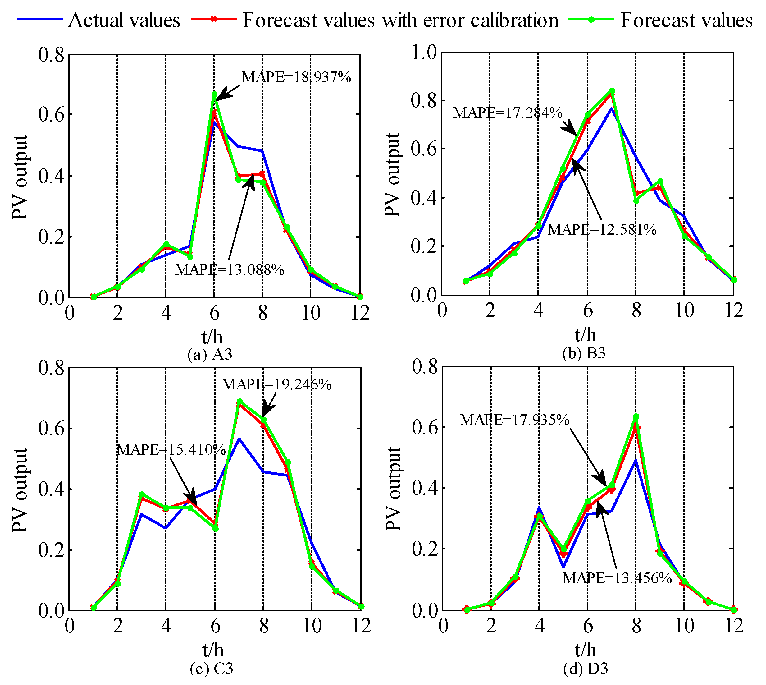
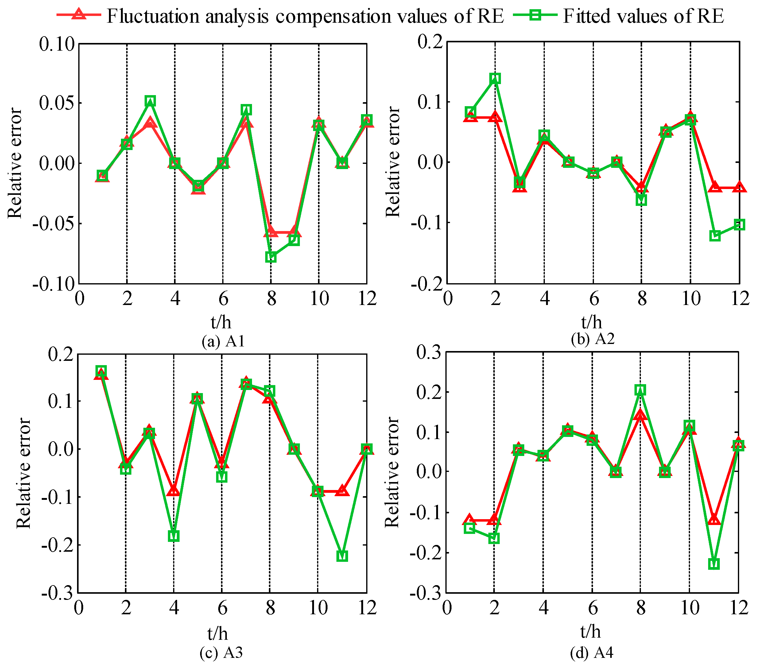
The probability density curves of the RE under each category are sampled based on a Latin hypercube sampling and a multi-scenario technique. Due to the low probability of the occurrence of large errors, the sections with peak values at their center with a probability of 85% are chosen to be the actual sampling intervals, in order to avoid the overcompensation of errors phenomenon caused by excessive sampling results. The sampling results of the RE are sorted according to the fluctuation analysis. The compensation error results and the final fitted values of the RE for A1–A4 are shown in
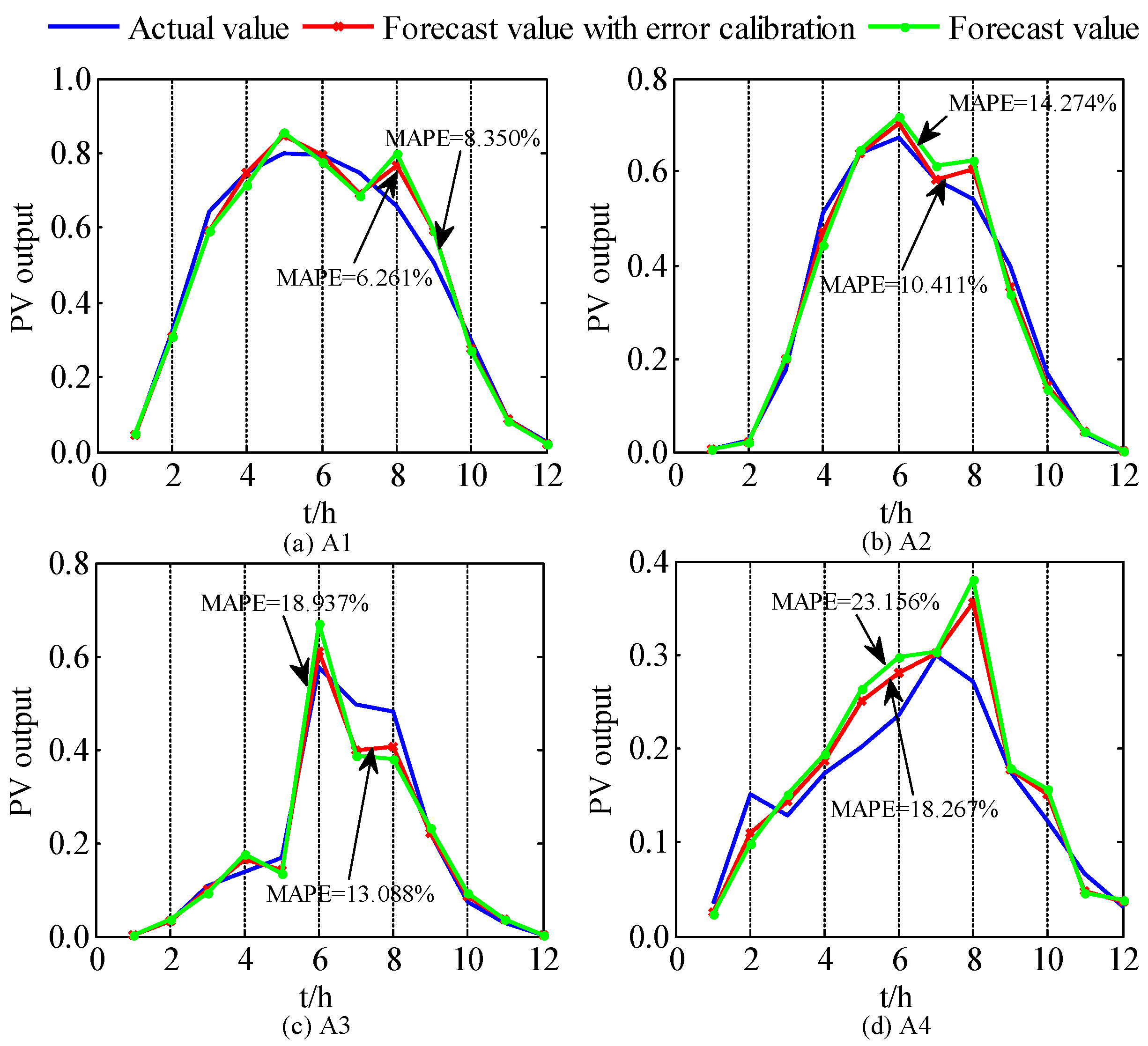
Figure 8. The forecasted results by the WNN with ADP are corrected by the fitted values of the RE to obtain the forecasted PV power output with error calibration. The final forecasted results for A1–A4 are shown in
Figure 9, and the forecasted results under the drizzle weather condition in each season are shown in
Figure 10. It is obvious from the two figures that after combining with an error calibration, the forecasting accuracy of each category can be improved to a certain extent.
Figure 8,
Figure 9 and
Figure 10 indicate that the fitted values of the RE can effectively eliminate the extreme values in the fluctuation analysis, aiming to avoid divergence and the overcompensation of error. Furthermore, the fluctuation analysis possesses the preliminary capacity of estimating the compensation values of the RE. Sorting the sampling error based on the compensation values, the forecasted PV power can corresponds correctly to the fitted RE. Due to the error calibration, the error can be compensated, and the forecasting accuracy can be improved.
7. Conclusions
In this paper, the function of a short-term PV power forecast based on the forecast error calibration and considering the typical climate categories is established. To begin with, the historical data of the PV power are sorted according to the typical climate categories. Then, the PDF curves for the RE of the PV power forecast are obtained for each category. An NKDE is utilized to develop the fitted PDF curves, and a Latin hypercube sampling along with a multi-scenario technique is used to obtain the sampling values of the RE. In addition, based upon a fluctuation analysis, the sampling values are sequenced by the compensation values of the RE, and the fitted values of the RE are generated. Finally, overly fit the values of the RE on the forecasted PV power values to improve the forecasting accuracy.
The results of the case study indicate the following.
- (1)
The RE data features of the PV power forecast noticeably vary between seasons and weather conditions. Based on the definition of the typical climate categories, the historical forecast error data were classified, which provides a good prerequisite for the establishment of probabilistic models and obtaining more accurate characteristics for the forecasting error.
- (2)
An NKDE with an optimal bandwidth could be applied to develop a probabilistic model in every typical climate category. An NKDE simulation fits better than a normal distribution simulation.
- (3)
By a fluctuation analysis, the rough compensation values for the RE of the PV power forecast are achieved, and according to which, the sampling values of the RE were consistent with the forecasted PV power. In contrast, the sampling values provide boundaries to the compensation values to avoid the overcompensation and divergence of error. The results of the case study demonstrated that by the means of simulating the forecast error of PV power based on its amplitude and fluctuation characteristics and then employing the fitted values of the RE to correct the PV forecast power, the prediction error can be reduced and the accuracy of the PV power forecast can be effectively improved.
Acknowledgments
The authors would like to acknowledge the Fundamental Research Funds for the Central Universities (2016ZZD07) and Beijing National Science Foundation (3164051).
Author Contributions
Jing Zhu carried out the main research tasks and wrote the full manuscript, and Yajing Gao proposed the original idea, analyzed and double-checked the results and the whole manuscript. Huaxin Cheng and Fushen Xue contributed to data processing and to writing and summarizing the proposed ideas, while Qing Xie and Peng Li provided technical and financial support throughout.
Conflicts of Interest
The authors declare no conflict of interest.
Abbreviations
The following abbreviations are used in this manuscript:
| PV | Photovoltaic |
| RE | Relative error |
| PDF | Probability density function |
| WNN | Wavelet neural network |
| NKDE | Nonparametric kernel density estimation |
| AMISE | Asymptotic mean integrated square error |
| IQR | Interquartile range |
| ADP | Adaptive dynamic programming |
| MAE | Mean absolute error |
| RMSE | Root mean square error |
| MAPE | Mean absolute percent error |
References
- Li, Z.; Rahman, S.M.; Vega, R.; Dong, B. A Hierarchical approach using machine kearning methods in solar photovoltaic energy production forecasting. Energies 2016, 9, 55. [Google Scholar] [CrossRef]
- Huld, T.; Amillo, A.M.G. Estimating PV module performance over large geographical regions: The role of irradiance, air temperature, wind speed and solar spectrum. Energies 2015, 8, 5159–5181. [Google Scholar] [CrossRef]
- Wang, F.; Mi, Z.; Su, S.; Zhao, H. Short-term solar irradiance forecasting model based on artificial neural network using statistical feature parameters. Energies 2012, 5, 1355–1370. [Google Scholar] [CrossRef]
- Sharma, V.; Yang, D.; Walsh, W.; Reindl, T. Short term solar irradiance forecasting using a mixed wavelet neural network. Renew. Energy 2016, 90, 481–492. [Google Scholar] [CrossRef]
- Larson, D.P.; Nonnenmacher, L.; Coimbra, C.F.M. Day-ahead forecasting of solar power output from photovoltaic plants in the American Southwest. Renew. Energy 2016, 91, 11–20. [Google Scholar] [CrossRef]
- Bridier, L.; Hernández-Torres, D.; David, M.; Lauret, P. A heuristic approach for optimal sizing of ESS coupled with intermittent renewable sources systems. Renew. Energy 2016, 91, 155–165. [Google Scholar] [CrossRef]
- Relevant statistical data of photovoltaic power in 2015. Available online: http://www.nea.gov.cn/2016-02/05/c_135076636.htm (accessed on 5 February 2016).
- Chen, C.; Duan, S.; Cai, T.; Dai, Q. Short-term photovoltaic generation forecasting system based on fuzzy recognition. Trans. China Electrotech. Soc. 2011, 26, 83–89. [Google Scholar]
- Wang, F.; Mi, Z.; Zhen, Z.; Yang, G.; Zhou, H. A classified forecasting approach of power generation for photovoltaic plants based on weather condition pattern recognition. Proc. CSEE 2013, 33, 57–64. [Google Scholar]
- Zhu, X.; Ju, R.; Cheng, X.; Ding, Y.; Zhou, H. Controller architecture design for MMC-HVDC physical simulation system. Autom. Electr. Power Syst. 2015, 39, 4–10. [Google Scholar]
- Dai, Q.; Duan, S.; Cai, T.; Chen, C.; Chen, Z.; Qiu, C. Short-term PV generation system forecasting model without irradiation based on weather type clustering. Proc. CSEE 2011, 31, 28–35. [Google Scholar]
- Yang, H.T.; Huang, C.M.; Huang, Y.C.; Pai, Y.S. A weather-based hybrid method for 1-day ahead hourly forecasting of PV power output. IEEE Trans. Sustain. Energy 2014, 5, 917–926. [Google Scholar] [CrossRef]
- Gao, Y.; Li, R.; Liang, H.; Zhang, J.; Ran, J.; Zhang, F. Two step optimal dispatch based on multiple scenarios technique considering uncertainties of intermittent distributed generations and loads in the active distribution system. Proc. CSEE 2015, 35, 1657–1665. [Google Scholar]
- Zhao, W.; Zhang, N.; Kang, C.; Wang, Y.; Li, P.; Ma, S. A method of probabilistic distribution estimation of conditional forecast error for photovoltaic power generation. Autom. Electr. Power Syst. 2015, 39, 8–15. [Google Scholar]
- Liu, D. A Model for Medium- and Long-Term Power Load Forecasting Based on Error Correction. Power Syst. Technol. 2012, 36, 243–247. [Google Scholar]
- Song, Y.; Shen, Z.; Dai, D.; Qian, Y.; Wang, Y. Short-term load forecasting in electrical power systems via trajectory tracking and error correcting approach. J. Renew. Sustain. Energy 2014, 6, 013112. [Google Scholar] [CrossRef]
- Sun, G.; Wei, Z.; Zhai, W. Short term wind speed forecasting based on RVM and ARMA error correcting. Trans. China Electrotech. Soc. 2012, 27, 187–193. [Google Scholar]
- Liu, W.; Yang, K.; Liu, D.; Hu, G. Day-ahead electricity price forecasting with error calibration by hidden Markov model. Autom. Electr. Power Syst. 2009, 33, 34–37. [Google Scholar]
- Ziadi, Z.; Oshiro, M.; Senjyo, T.; Yona, A.; Urasaki, N.; Funabashi, T.; Kim, C.H. Optimal voltage control using inverters interfaced with PV systems considering forecast error in a distribution system. IEEE Trans. Sustain. Energy 2014, 5, 682–690. [Google Scholar] [CrossRef]
- Lin, S.; Han, M.; Zhao, G.; Niu, Z.; Hu, X. Capacity allocation of energy storage in distributed photovoltaic power system based on stochastic prediction error. Proc. CSEE 2016, 36, 692–700. [Google Scholar]
- China Meterological Administration. GB/T 22164—2008 Public Climate Service—Weather Graphic Symbols; Standards Press of China: Beijing, China, 2008.
- Gao, Y.; Cheng, H.; Zhu, J.; Liang, H.; Li, P. The Optimal Dispatch of a Power System Containing Virtual Power Plants under Fog and Haze Weather. Sustainability 2016, 8, 71. [Google Scholar] [CrossRef]
- Yan, W.; Ren, Z.; Zhao, X.; Yu, J.; Li, Y.; Hu, X. Probabilistic photovoltaic power modeling based on nonparametric kernel density estimation. Autom. Electr. Power Syst. 2013, 37, 35–40. [Google Scholar]
- Ye, A. Nonparametric Econometrics; Nankai University Press: Tianjin, China, 2003. [Google Scholar]
- Epanechnikov, V.A. Nonparametric estimation of a multidimensional probability density. Theory Probab. Appl. 1969, 14, 153–168. [Google Scholar] [CrossRef]
- Silverman, B.W. Density Estimation for Statistics and Data Analysis; Chapman and Hall: London, UK, 1986. [Google Scholar]
- Pholdee, N.; Bureerat, S. An efficient optimum Latin hypercube sampling technique based on sequencing optimisation using simulated annealing. Int. J. Syst. Sci. 2015, 46, 1780–1789. [Google Scholar] [CrossRef]
- Li, Z.; Floudas, C.A. Optimal Scenario Reduction Framework based on Distance of Uncertainty Distribution and Output Performance: II. Sequential Reduction. Comput. Chem. Eng. 2015, 84, 599–610. [Google Scholar] [CrossRef]
- Ye, L.; Ren, C.; Zhao, Y.; Rao, R.; Teng, J. Stratification analysis approach of numerical characteristics for ultra-short-term wind power forecasting error. Proc. CSEE 2016, 36, 692–700. [Google Scholar]
- Gao, Y.; Liu, D.; Cheng, H.; Li, T.; Li, P. Predictor-corrector model of wind power forecast based on data-driven. Proc. CSEE 2015, 35, 2645–2653. [Google Scholar]
© 2016 by the authors; licensee MDPI, Basel, Switzerland. This article is an open access article distributed under the terms and conditions of the Creative Commons Attribution (CC-BY) license (http://creativecommons.org/licenses/by/4.0/).


