Curtailment in a Highly Renewable Power System and Its Effect on Capacity Factors

Abstract

The capacity factor of a power plant is the ratio of generation over its potential generation. It is an important measure to describe wind and solar resources. However, the fluctuating nature of renewable power generation makes it difficult to integrate all generation at times. Whenever generation exceeds the load, curtailment or storage of energy is required. With increasing renewable shares in the power system, the level of curtailment will further increase. In this work, the influence of the curtailment on the capacity factors for a highly renewable German power system is studied. An effective capacity factor is introduced, and the implications for the distribution of renewable power plants are discussed. Three years of highly-resolved weather data were used to model wind and solar power generation. Together with historical load data and a transmission model, a possible future German power system was simulated. It is shown that effective capacity factors for unlimited transmission are strongly reduced by up to 60% (wind) and 70% (photovoltaics) and therefore of limited value in a highly renewable power system. Furthermore, the results demonstrate that wind power benefits more strongly from a reinforced transmission grid than photovoltaics (PV) does.

1. Introduction

The German Energiewende is the process that dispatchable conventional generation units in Germany are replaced by generation from renewable sources. The share of renewable generation in the electricity mix has increased in Germany from 6.3% in 2000 to 29.7% for the first eleven months of 2014 [1]. This 29.7% is divided into 9% wind power, 6.9 % photovoltaics (PV), 3.6% hydro and 10.2% biomass. Concerning the net installed capacities, wind and PV are the leading technologies with 35.6 GW wind (including 0.6 GW offshore) and 38.1 GW PV. Wind and PV are usually considered the most promising renewable technologies for energy generation in the world [2,3]. However, the strongly fluctuating and non-controllable nature of renewable power sources makes the system integration difficult (despite the spatial smoothing of wind [4] and PV [5] feed-in).

The capacity factor of a power plant is the ratio between its actual output in a period of time over the maximal theoretical output in the same period [6]. It is an important measure to decide on new sites for further deployment of renewable energy sources and to derive an optimal wind turbine layout for a specific site [7]. Furthermore, it can also be computed for an ensemble of power plants or an entire country and has direct influence on the financial performance of renewable power plants [8]. For wind turbines, the capacity factor is determined mainly by the geographic location of the wind turbine, as well as the turbine design itself. This renders the absolute value of the capacity factor for a site somewhat arbitrary. One might imagine a small generator combined with a very large rotor leading for most locations to an extremely high capacity factor. Consequently, the technical assumptions are fixed throughout the paper. Details are given in Section 3. For renewable sources, the capacity factor highly relies on meteorological conditions and is therefore also referred to as the meteorological capacity factor. However, for very high shares of renewables and therefore increased curtailment, this capacity factor seems not sufficient to describe the resource of a site adequately. This leads to the introduction of the effective capacity factor. This modified capacity factor considers only generation that is really used and not curtailed. This means that the interplay of generation at different locations and the load patterns need to be taken into account. The effect of curtailment on capacity factors was already discussed for the U.S. without transmission constraints in [9]. Curtailment of wind power induced by congestion was discussed in [10]. The work in [11] introduced the idle capacity as a measure for ineffectively deployed wind power capacity and connected it to several socio-economic factors. However, this work focuses on socio-economic aspects.

Germany is still far from a dominance of fluctuating renewables on the generation side. Nevertheless, a renewable share in the electricity mix of 100% is possible by 2050 [12]. In addition, recent numbers for Germany published by the Bundesnetzagentur (Federal Network Agency) [13] show that curtailment is an issue already: although the share from renewable sources in the electricity mix was below 30% in 2014, 1.6 TWh of wind/PV and biomass generation (ca. 1.2% of total generation from these sources) were curtailed. This was explained to be mainly due to wind power generated in the north not being able to reach the south due to congestion. In comparison to 2013, this value has tripled and demonstrates that curtailment can even be of some importance if renewable shares of generation are rather low.

Furthermore, several events of curtailment of renewable generation have been reported across Europe in the past few years: The economic impact of curtailment in Spain was described as a loss of approximately 70 million Euro from January to March 2013, and the amount of curtailment is expected to increase to yearly 2.3 TWh (3.1% of renewable generation) in 2020 [14]. In Italy, the amount of curtailed wind energy was reduced from 10.7% in 2009 to 1.24% in 2013 due to a significant reinforcement of the transmission grid capacities. In Ireland, 110 GWh wind energy were curtailed in the year 2012 [15]. This is approximately 2% of the total wind generation. Congestion in the power transmission system was responsible for about 80% of the losses, while 20% was due to local network constraints.

The main objective of this paper is to demonstrate the large reduction of the capacity factor due to curtailment in a highly renewable power system and the therefore questionable relevance of the meteorological capacity for site assessment. For this purpose, the following steps are taken: (1) the introduction of an effective capacity factor as an alternative to the meteorological capacity factor; (2) the computation of the effective capacity factors for two highly renewable scenarios of the future German power system; (3) investigation of the dependency of the effective capacity factor on the capacity distribution and the transmission grid strength; (4) drawing of conclusions from the investigation: what does curtailment imply for the preferable design of the future German power system with a very high share of renewables?

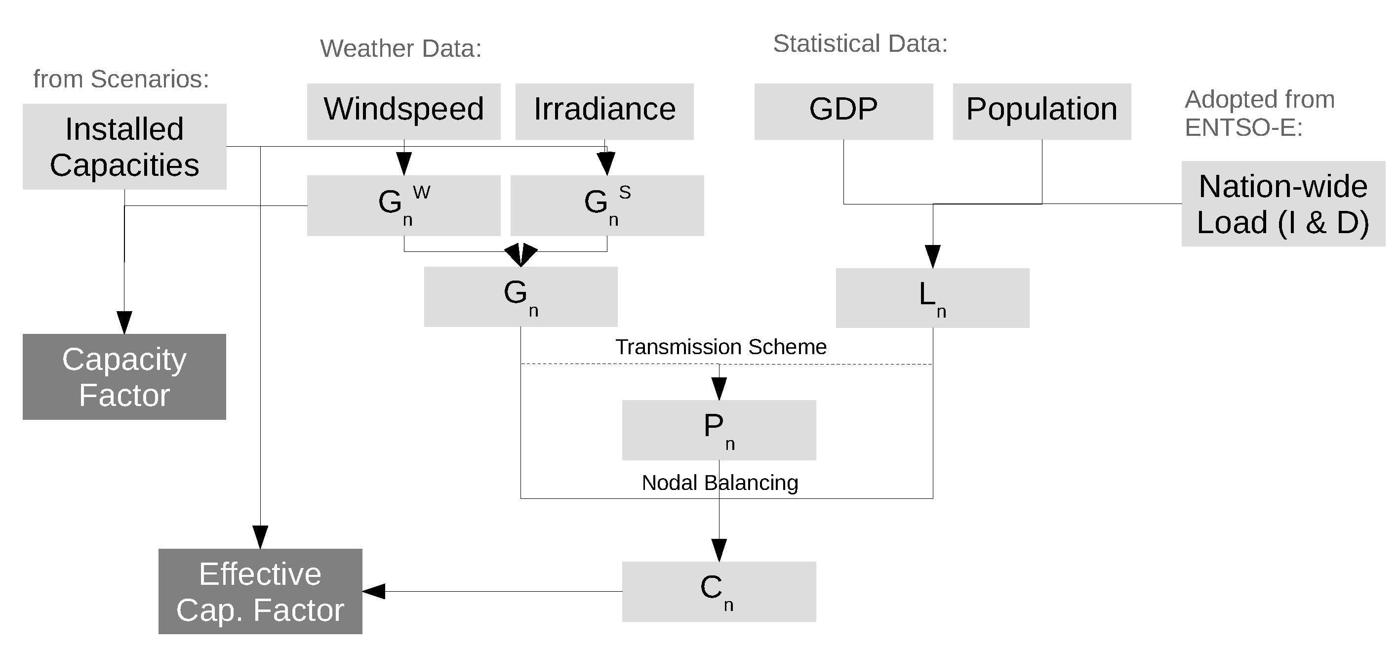
2. Methodology

A possible future German power system is simulated. Counties (and independent cities, also referred to as counties) are considered as generators and consumers and represent the nodes in the system, which are connected by links. To derive the grid topology, the simple assumption is made that every county is connected to its direct neighbors via a link of length $d_l$ (average length: 33.5 km), where the length is given by the distance between the geographical centers. Hence, the power grid consists of 402 nodes and 1049 links (Figure 1).

The counties themselves are assumed to be ideal nodes. In existing systems, transmission losses are usually small (1%–2% per 100 km at 380 kV [18]) and neglected. This model setup has been chosen for the following reasons: Firstly, the transmission system should impose as little restrictions as possible on the exchange of energy within the system. An even larger system with more nodes and links, however, would become increasingly computationally expensive and numerically unstable. Secondly, counties are the political-administrative entity responsible for transmission grid planning, supervision and approval.

Two major restrictions apply to the model: first, offshore wind is not considered, and second, Germany is investigated as an isolated power system. These restrictions are briefly discussed in Section 5. For the following investigation, time series of generation for wind $W_n(t)$ and PV $S_n(t)$, based on highly resolved weather data, were computed for each node. Together, they compose the generation of the node n,

$$\begin{array}{cc}\hfill G_n(t)& =W_n(t)+S_n(t)\hfill \end{array}$$

(1)

The corresponding time series of the mismatch between generation and load is:

$$\begin{array}{cc}\hfill {\Delta }_n(t)& =G_n(t)-L_n(t)\hfill \end{array}$$

(2)

or, if transmission is included,

$$\begin{array}{cc}\hfill {\Delta }_n(t)& =G_n(t)-L_n(t)+I_n(t)-E_n(t)\hfill \end{array}$$

(3)

where $L_n(t)$ is the time series of the load, $E_n(t)$ are the exports and $I_n(t)$ are the imports of node n. At each node and at all times, generation must equal load to ensure the stability of the system. This leads to the nodal balancing equation:

$$\begin{array}{cc}\hfill G_n(t)-L_n(t)& =P_n(t)-B_n(t)+C_n(t)\hfill \end{array}$$

(4)

where $P_n(t)$ is the injection pattern (imports-exports), $B_n(t)$ is the backup (i.e., dispatchable generation) and $C_n(t)$ is curtailed excess energy. Throughout the paper, it is assumed that excess energy is curtailed, and remaining residual loads are covered by backup energy. It follows directly that backup and curtailment do not occur at the same node for the same time. Backup power is not explicitly investigated in the following, since this investigation focuses on the aspect of curtailment. The curtailment time series is calculated as:

$$\begin{array}{cc}\hfill C_n(t)& =max\left(\{0,{\Delta }_n(t)\}\right)\hfill \end{array}$$

(5)

where ${\Delta }_n(t)$ is the mismatch after transmission. The left part of the balancing Equation (4) is the active part that is determined by the given data, while the right side is the reactive part, i.e., the response of the system. More generally, this equation could be extended by additional terms to account for storage, demand side management, etc. The transmission model, which determines the injection pattern, is described in Section 2.2. After generation, load and transmission, the remaining residual mismatch is handled by either the backup (if ${\Delta }_n<0$, i.e., energy deficit) or curtailment (if ${\Delta }_n>0$, i.e., energy excess).

2.1. Definitions

In a given county, the ratio of average renewable generation to average load is described by the share of renewables ${\alpha }_n$,

$$\begin{array}{cc}\hfill {\alpha }_n& =\frac{〈G_n(t)〉}{〈L_n(t)〉}\hfill \end{array}$$

(6)

Equivalently, the share of renewables of the whole system is given by:

$$\begin{array}{c}\hfill \alpha =\frac{〈G(t)〉}{〈L(t)〉}=\frac{{\sum }_n〈G_n(t)〉}{{\sum }_n〈L_n(t)〉}\end{array}$$

(7)

For $\alpha =1.0$, the generation in all counties combined is on average equal to the average load combined. In this paper, only $\alpha =1.0$ is considered. Besides α, the parameter β describing the solar share in the renewable generation is defined as:

$$\begin{array}{cc}\hfill {\beta }_n& =\frac{〈G_n^S(t)〉}{〈G_n^S(t)+G_n^W(t)〉}\hfill \end{array}$$

(8)

and similarly for the whole system. For a highly renewable European power system, the optimal β was found to be around 0.4 with respect to the standard deviation of the mismatch [19] or around 0.2 with respect to the need for balancing energy [20].

The capacity factor is the major terminology of this study. For a given county, it is defined as:

$$\begin{array}{cc}\hfill {\nu }_n^{w/s}& =\frac{〈G_n^{w/s}(t)〉}{〈G_{n,nom}^{w/s}〉}\hfill \end{array}$$

(9)

where $〈G_{n,nom}^{w/s}〉$ is the rated power. Consequently, the effective capacity factor for wind ${\tilde{\nu }}^w$ and photovoltaics ${\tilde{\nu }}^s$ is defined by:

$$\begin{array}{c}\hfill {\tilde{\nu }}_n^{w/s}={\nu }_n^{w/s}\left(1-\frac{〈C_n^{w/s}(t)〉}{〈G_n^{w/s}(t)〉}\right)\end{array}$$

(10)

This definition of an effective capacity is similar to the definition of idle capacity in [11]. Note that the effective capacity factor is the capacity factor that only counts the energy consumed either locally or after transmission.

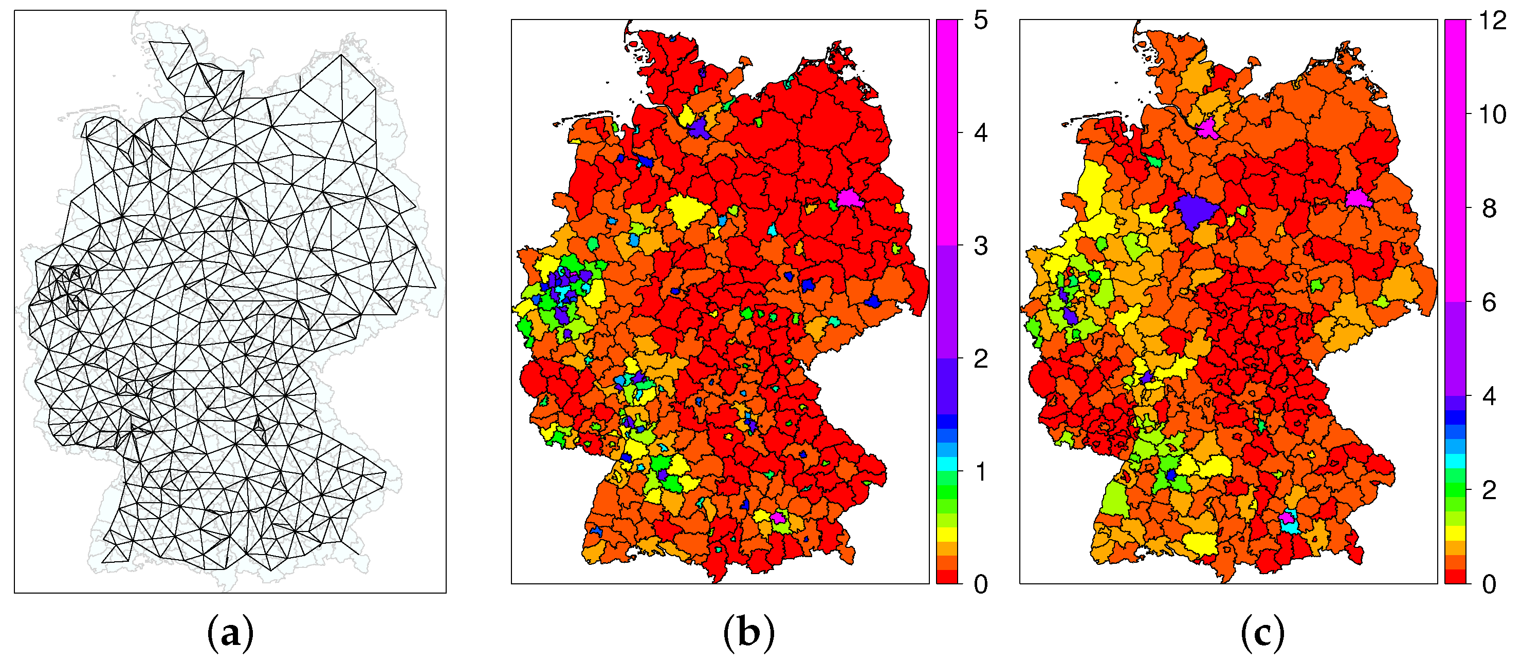
2.2. Transmission

Transmission is modeled as a two-step optimization problem for every time step. The equations of the full electric power-flow in an AC electricity network are used in a common DC approximation. For a full derivation of this DC approximation, see, for example, [21,22]. In the first step, the total backup energy is minimized:

$$\begin{array}{cccc}\underset{F_l}{\text{minimize}}\hfill & & \sum _n{B}_n(t)=:B^{\text{min}}(t)\hfill & (11)\\ \text{subject}\text{to}\hfill & & F_l^{-}\le F_l\le F_l^{+}\hfill & (12)\end{array}$$

where $F_l^{\pm }$ are the transmission capacities of link l in both directions. This optimization does not necessarily result in a unique solution for the flows $F_l$. Therefore, the uniqueness of the solution is ensured by minimizing the dissipation ${\sum }_l{d}_l{F}_l^2$, while keeping the overall backup energy need $B^{\text{min}}(t)$;

$$\begin{array}{cccc}\underset{F_l}{\text{minimize}}\hfill & & \sum _l{d}_l{F}_l^2\hfill & (13)\\ \text{subject}\text{to}\hfill & & F_l^{-}\le F_l\le F_l^{+}\hfill & (14)\\ & & \sum _n{B}_n(t)=B^{\text{min}}(t)\hfill & (15)\end{array}$$

where $d_l$ is the length of link l. The injection pattern $P(t)$ is afterwards calculated via the unique solution for the flows $F_l$ of the optimization,

$$\begin{array}{cc}\hfill P_n& =\sum _l{K}_{nl}{F}_l\hfill \end{array}$$

(16)

K is the incidence matrix, whose elements are defined by:

$$\begin{array}{c}\hfill K_{nl}=\left\{\begin{array}{cc}1\hfill & \text{if link l begins at node n}\hfill \\ -1\hfill & \text{if link l ends at node n}\hfill \\ 0\hfill & \text{otherwise}\hfill \end{array}\right.\end{array}$$

(17)

An equivalent transmission model is used in [23,24,25,26,27,28,29]. The effectively-used transmission capacity ${\kappa }_l^T$ of a link l connecting two nodes is defined by the 99th percentile,

$$\begin{array}{cc}\hfill 0.99& ={\int }_0^{{\kappa }_l^T}p(|F_l|)dp\hfill \end{array}$$

(18)

where $p(|F_l|)$ is the time sampled distribution of the absolute values of the unlimited flow over the link l. The transmission capacity of every single link is thus sufficient 99% of the time. This means a transmission grid where every link has the capacity computed by Equation (18) is assumed to be the grid required for unlimited transmission (under the minor restriction that it uses the 99th percentile). Using the 99th percentile for the definition of the transfer capacities aims at reducing the sensitivity towards the weather database.

2.3. Scenario Definition

The following two 100% renewable scenarios (i.e., $\alpha =1$) were defined for this study:

• Wind and PV capacities are distributed in such a way that ${\alpha }_n=\alpha =1$. This means that every county produces on average as much renewable energy as it consumes.
• For every county, the currently-installed capacity of wind and PV (2013) is multiplied with the same factor. In this case, today’s spatial distribution of capacities is kept, but every installed wind turbine or PV module is upgraded by a certain factor. This process is usually referred to as repowering.

The solar share ${\beta }_n$ (see Equation (8)) is fixed for all German counties as it was at the end of 2013. ${\beta }_n$, and the capacity densities for wind and PV can be seen in Figure 2. In northern Germany, ${\beta }_n$ is marginal and approaches unity in southern Germany. In the following, the first scenario is referred to as the self-sufficient scenario, while the second is called the upscaled scenario. The key characteristics of both scenarios can be seen in

Table 1. Summary of the main differences between the scenarios for unlimited transmission.

Scenario	β	$〈\frac{{\mathit{C}}^{\mathit{w}}}{{\mathit{G}}^{\mathit{w}}}〉$	$〈\frac{{\mathit{C}}^{\mathit{s}}}{{\mathit{G}}^{\mathit{s}}}〉$	$〈\frac{\mathit{C}}{\mathit{G}}〉$	${\mathit{C}\mathit{a}\mathit{p}}^{\mathit{w}}$ (GW)	${\mathit{C}\mathit{a}\mathit{p}}^{\mathit{s}}$ (GW)	${\sum }_{\mathit{l}}{\mathit{d}}_{\mathit{l}}{\mathit{\kappa }}_{\mathit{l}}^{\mathit{T}}$ (GWkm)
Self-Sufficient	0.68	0.14	0.52	0.39	160	389	13,800
Upscaled	0.35	0.27	0.29	0.28	289	206	27,065

(Section 4). One-hundred percent of generated electricity by 2050 from renewable sources in Germany is in line with a statement of the German Advisory Council on the Environment (SRU) [12]. Thus, the aforementioned scenarios of capacity distribution might be realized at that point. Obviously, they represent the most extreme cases (repowering of all existing generation facilities vs. a homogenous distribution). Thus, the deployment will likely be in between these scenarios by 2050. Figure 3 depicts the general proceeding of this study. The optimization steps were performed using the Python API of Gurobi.

3. Data

Curtailment is determined by the interplay of generation and load, as well as by the given possibilities to balance mismatches by importing and exporting energy, i.e., using the grid. To model renewable generation from wind and PV, three years of highly resolved weather data were used. The used data period ranges from January 2010 to December 2012. Wind speeds and irradiance are converted to generation by state-of-the-art methods that are described in more detail in this section.

3.1. Weather Data

Computations of generation are based on data from the following sources:

• Wind speed data at hub height of 77 m and 2-m temperature data from the analysis product of the numerical weather prediction model (NWP) COSMO-DE [30], provided by the German Weather Service (Deutscher Wetterdienst, DWD) and
• Solar irradiation data from Meteosat Second Generation (MSG).

COSMO-DE data have a spatial resolution of $0.025$° (ca. 3 km) and hourly temporal resolution. The model domain is centered over Germany and consists of $461\times 421$ grid cells. The satellite data were used with a spatial resolution of $0.0625$° (ca. 7 km).

3.2. Generation Data

The weather data described in the previous section are used to compute generation time series from wind and PV for each of the 402 German counties. For wind power, the hub height is assumed to be 77 m, the average hub height of wind power plants in Germany at the end of 2013. In the past few years, a trend towards increasing hub heights was observed. Thus, it is likely that the average hub height will increase further leading to higher capacity factors for better wind regimes at these heights. However, this mainly affects the absolute value of the capacity factor. The effect on relative changes due to curtailment are assumed to be negligible.

Wind speeds are converted to power via the power curve model described in [31]. This power curve was fitted to obtain the best match of simulated and observed wind power in the largest German transmission grid zone. We use data for the geographical distribution of installed wind and PV capacities from 2013. For PV power generation, the Klucher model [32] is used to model irradiation on the inclined surface. The PV modules are assumed to have a tilt of 30° and a south-facing orientation (azimuth = 0°). Module temperatures were computed as:

$$\begin{array}{cc}\hfill T_m& =T_a+\sigma I_t\hfill \end{array}$$

(19)

where $T_a$ is the ambient temperature, $T_m$ the module temperature and $I_t$ the irradiance on the inclined surface. σ is a factor that was chosen to be $0.036\frac{{\text{km}}^2}{\mathrm{W}}$. The module efficiency $\eta (T_m)$ is calculated as a function of the module temperature,

$$\begin{array}{cc}\hfill \eta (T_m)& =\eta (25°)\left(1+a{T}_m\right)\hfill \end{array}$$

(20)

where $a\in R$ is device-specific. DC power can then be calculated by using the installed capacity,

$$\begin{array}{cc}\hfill P& =\eta (T_m)I_t{\text{Cap}}^s\hfill \end{array}$$

(21)

for any grid point. DC power was converted into AC power using the parameters of a Sunny Mini Central 8000 TL converter [33]. Generation for wind and PV is calculated on the grid point level and aggregated to counties afterwards.

3.3. Load Data

Historical load data for Germany provided by the European Network of Transmission System Operators for Electricity (ENTSO-E) was taken. These data were modified within the RESTORE2050 project (Frank Merten, Wuppertal Institute, private communication via e-mail, 2014). Modifications include modeled load profiles from e-mobility and heat pumps.Since no information about the energy demand on a sub-national level is publicly available in Germany, load time series of the counties are estimated based on the county’s gross domestic product GDP${}_n$ and on the county’s number of inhabitants $D_n$; $L(t)=L_D(t)+L_I(t)$ is the modified ENTSO-E load time series for the entirety Germany, consisting of a domestic and an industrial part. The total load of county n, $l_n$, is expressed as:

$$\begin{array}{c}\hfill l_n(t)=l_{I,n}(t)+l_{D,n}(t)\end{array}$$

(22)

where $l_{I,n}$ and $l_{D,n}$ are the industrial and domestic load time series, respectively. The partial loads are computed as:

$$\begin{array}{cc}\hfill l_{I,n}(t)& ={\text{GDP}}_n·\frac{L_I(t)}{{\sum }_n{\text{GDP}}_n}\hfill \end{array}$$

(23)

$$\begin{array}{cc}\hfill l_{D,n}(t)& =D_n·\frac{L_D(t)}{{\sum }_n{D}_n}\hfill \end{array}$$

(24)

The population density and the gross domestic product of the German counties can be seen in Figure 1 (center and right) for 2012. GDP per capita tends to increase from north to south and from east to west.

4. Results

The results Section is structured as follows: First, capacity factors are calculated from the meteorological data alone. Second, the effective capacity factors are calculated. The dependency on the share of renewables, the solar share and the transmission grid capacities are discussed in Section 5.

Table 1 shows the shares of wind and PV power in the electricity mix, as well as the resulting major quantities, like curtailment and transmission capacity needs for both investigated scenarios. The transmission capacities are determined according to Equation (18) for every link and multiplied with the corresponding length $d_l$. Thus, the displayed values show the need for unlimited transmission as defined by the 99th percentile in this work. In the self-sufficient scenario, every county produces on average as much as it consumes, leading to a very homogenous distribution of generation facilities in Germany. This is reflected by the fact that the self-sufficient scenario has a much lower demand for transmission grid capacities, which is about half the need of the upscaled scenario. In turn, needed generation capacities are around 10% less, and only 28% of the generation is curtailed in the upscaled scenario (39% in the self-sufficient scenario).

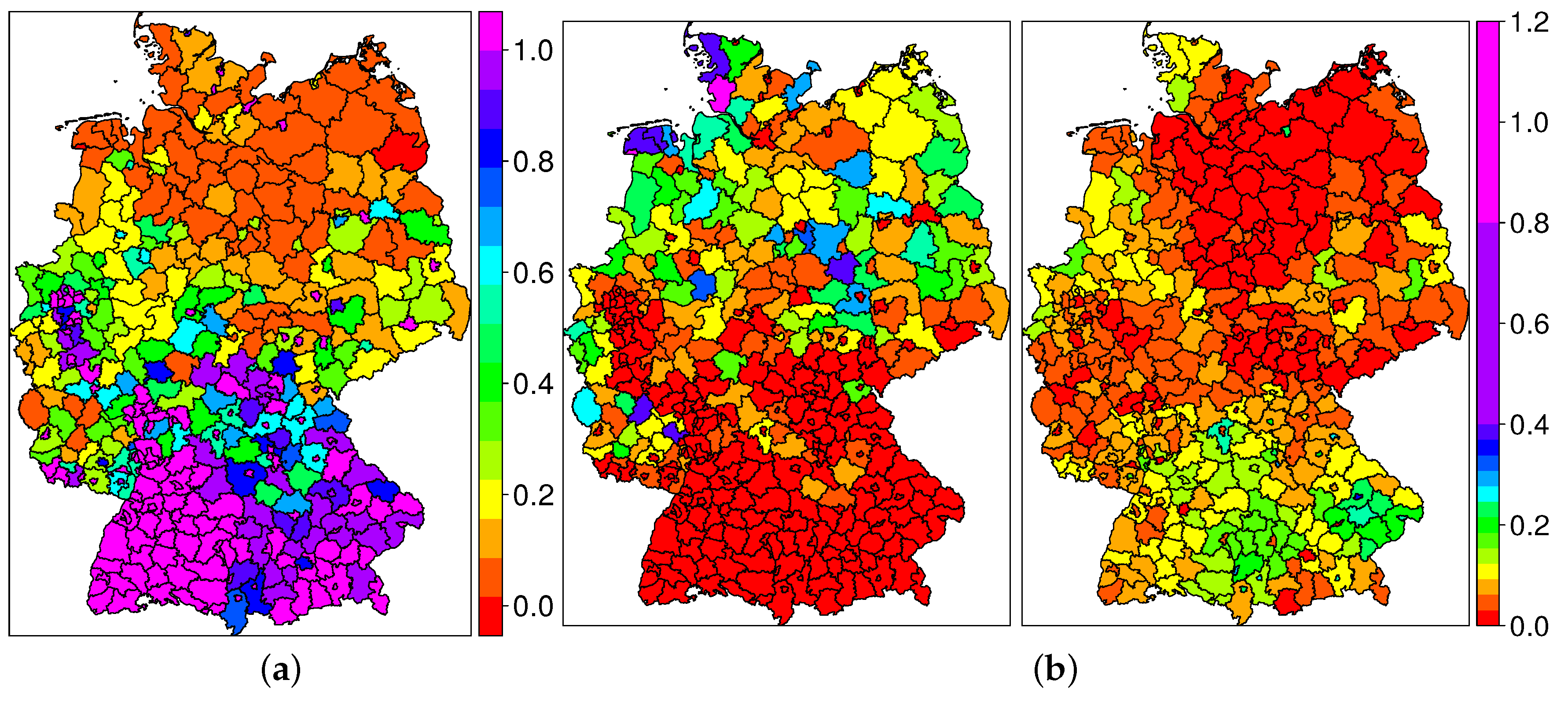
4.1. Meteorological Capacity Factors

The meteorological capacity factor of a renewable power plant (often simply referred to as the capacity factor) is the actual output in a certain period of time over its theoretical output. The theoretical output is defined by the rated power of the generation unit, for example the wind turbine or PV module. These meteorological capacity factors were calculated under the technical specifications described in Section 3 for every county and are shown in Figure 4. For wind, they are strongly increasing up north, while the opposite is true for PV. Capacity factors for wind power plants are around 20% in the northern part of Germany, but only around 10% in southern Germany. Capacity factors for PV vary less, reaching around 14% in southern Germany and 10% in northern Germany. Total capacity factors for wind and PV in Germany are found to be 16.1% and 12.3% for the upscaled scenario, respectively. This compares to the capacity factors published by the German Federal Ministry of Economic Affairs and Energy for the years 2010 to 2012 of $17.9$% for onshore wind and of $8.6$% for PV [34]. The small apparent discrepancy is likely caused by the technological assumptions made in this study (note: the capacity distribution used is the actual capacity distribution of today and can therefore not be responsible for the differences observed).

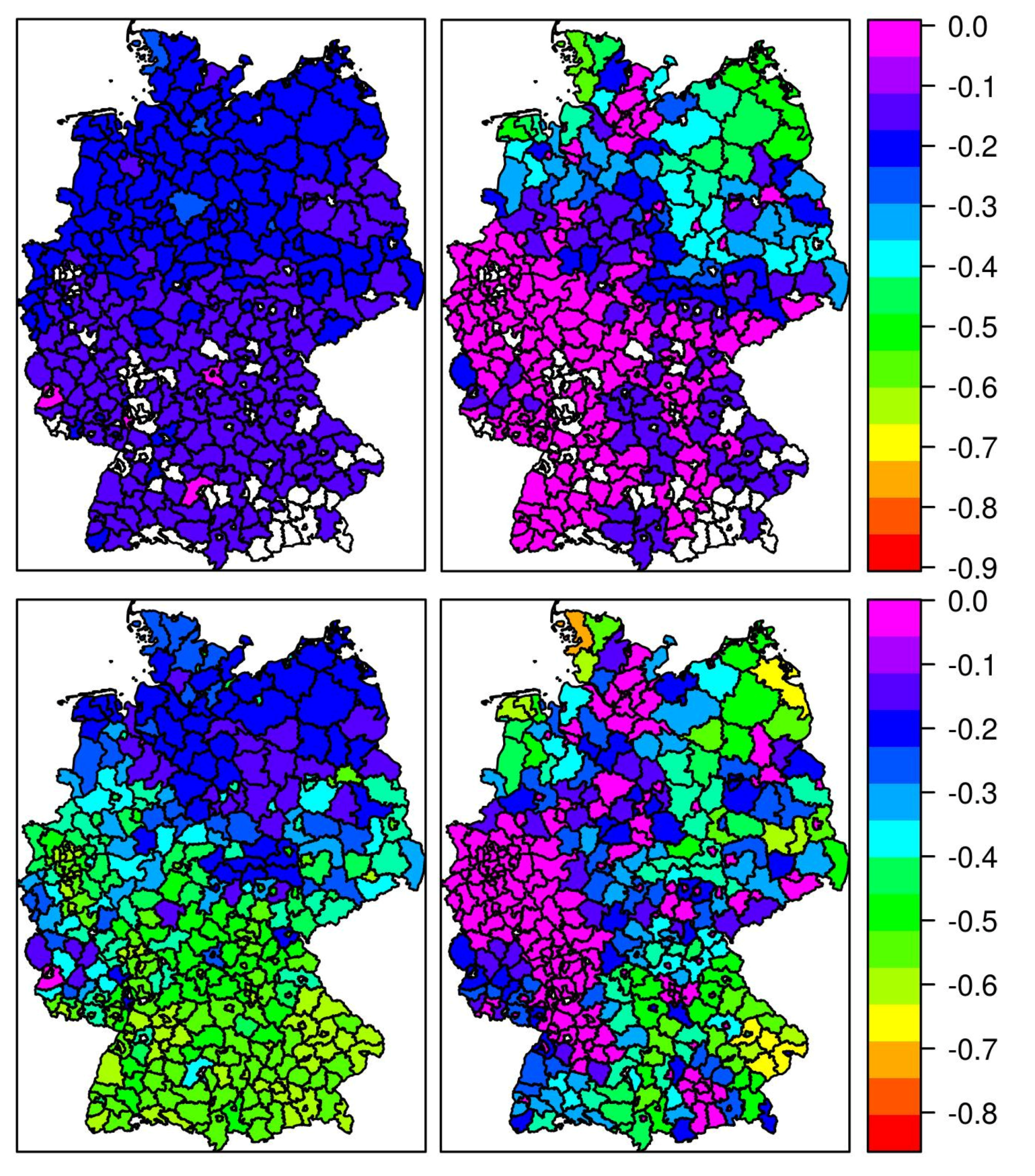
4.2. Effective Capacity Factors

In contrast to the meteorological capacity factors, the effective capacity factor measures only the power output that is effectively used. As they were introduced in Section 2.3, effective capacity factors ${\tilde{\nu }}^{w/s}$ (see Equation (10)) are investigated for two scenarios of capacity distribution. In the self-sufficient scenario, the effective capacity factors are reduced to 6% to 20% for wind and 5% to 12% for PV (Figure 5). While the general qualitative distribution of the effective capacity factor remains for wind (high values in the north and low values in the south), it changes considerably for PV. A strong relationship between the change from ${\nu }^s$ to ${\tilde{\nu }}^s$ and the share of PV β exists. The highest values for ${\tilde{\nu }}^s$ can be found towards the northwest and in the central German regions, i.e., in regions with relatively low β (see Figure 2, left). On the contrary, in urban areas of western Germany and in the south, i.e., the regions where the highest meteorological capacity factors and the highest shares of PV occur, the effective capacity factors decrease the most compared to the meteorological capacity factors.

In the upscaled scenario, effective capacity factors range from 10% to 15% for wind and from 3% to 13% for PV. The strongest reduction for both wind and PV occurs in the rural areas in northeastern and southeastern Germany, as well as the coastal regions. In urban areas and their direct surroundings, the differences between capacity factors and effective capacity factors for PV are very small. For wind the north-south gradient disappears in almost all regions. The high amount of produced power in northern regions leads to strong curtailment and therefore largely reduced capacity factors.

5. Discussion

Where does curtailment occur and why? This paper revolves around the idea of the meteorological capacity factor being no appropriate measure to describe the quality of a site, if shares of renewables are high and thus events of curtailment common. This is closely linked to the problem of decoupled generation and transmission in the power market leading to suboptimal investment choices [35,36,37,38].

At what locations does curtailment occur? This depends on different aspects, like the electricity market and the transmission grid. Today, transmission system operators decide on curtailment, and affected owners are almost fully compensated in Germany [39]. The cost of curtailment events are therefore borne by the consumers as a lump sum via network access charges (Netznutzungsentgelte). However, this might change in the future, rendering the question of curtailment more important for the operational side. The coalition agreement of the present German Federal Government aims at modifying the compensation for curtailment so as to provide more incentive to consider the grid situation for new renewable power plants [40].

The markets plays a role mainly via the question of how the cost of transmission is distributed among the market participants. Consider the simple three-node example shown in Figure 6. The three nodes {A,B,C} are connected via two links from A to B and B to C. A and B have similar marginal generation cost and place offers. C bids. If transmission cost does not add to the marginal cost by being provided independently and offers are pooled (shared among market participants), Scenario (II) is realized: A and B both transfer half of their excess energy to C, thus curtailing the other half. If instead transmission cost is above zero and included in the marginal cost, Scenario (III) is realized. B transfers its excess energy to C, and A curtails its power. To generalize this idea: for generation at topologically-favorable positions in the network, marginal costs are comparably low, and curtailment is less likely than at nodes at less favorable positions.

How does the market model connect to the abstract grid topology of this paper? It was assumed that every county is connected to its neighbors. Obviously, this does not resemble today’s historically grown power grid. Today, it connects regions and their distribution grids via the high voltage transmission grid. However, the authors of this paper believe that the detailed topology of the grid becomes less important, if the transmission grid is strongly reinforced. In addition, the optimal topology for a highly renewable grid still needs to be determined and will likely differ to some extent from the grid Germany has today. Therefore, it is likely that the beneficial positions in the grid with respect to curtailment will be less dependent on today’s grid. Instead, it will heavily depend on the geographical location (distance to load centers). In that way, the chosen abstract topology can be justified.

Two major restrictions apply to the model: offshore wind is not considered, and Germany is investigated as an isolated power system. The first point is probably the less problematic one. The largest differences between meteorological and effective capacity factors, as described in the following sections, are observed in the northernmost regions. These regions border the German offshore regions, which implies that the results would be even more prominent, if offshore wind power generation were included. Concerning imports and exports: under the transmission scheme applied in this paper, it is shown in [23] that Germany imports and exports (for a share of renewables in Germany and Europe: 70%) ca. 7% in units of its consumption. Under the methodology of this investigation, imports can increase curtailment while exports can reduce curtailment. Therefore, it might be an interesting extension of this work to embed Germany into a fully renewable European power system and to study the effect of this on the effective capacity factors.

5.1. Wind/PV Ratio

The results indicate that the wind/PV mix of a node has a large effect on the effective capacity factor. This is easily understandable: The wind/PV ratio determines the temporal correlation of generation and load, which, in turn, has a strong impact on the curtailment. Besides, PV power has a strong diurnal pattern and therefore resembles to some extent the typical diurnal load pattern (peaks during the day and minima at night). On the contrary, wind power generation only exhibits a very weak diurnal cycle. Figure 7 summarizes the reduction of the capacity factor,

$$\Delta {\nu }^{w/s}=\frac{{\tilde{\nu }}^{w/s}-{\nu }^{w/s}}{{\nu }^{w/s}}$$

(25)

for the four quartiles $[0,Q1],...,(Q3,1]$ of the solar share β. Focusing on wind, several things can be observed: the largest reduction of capacity factors occurs in the upscaled scenario and for small β, i.e., in counties with high shares of wind power generation. In the case of limited transmission (definition in Section 5.3), shown as yellow boxes, this reduction amounts up to 80%. In the self-sufficient scenario, the difference between the different intervals of β is minor, i.e., the ratio between PV power and wind power generation is not the driving factor here. The difference between the two scenarios can be explained by the fact that wind power generation accounts for ca. two thirds of total power generation in the upscaled scenario, while it contributes only one third in the self-sufficient case. Furthermore, the correlation between the mismatch of the county and the overall mismatch is relatively high in counties with high shares of wind leading to much curtailment in these counties.

For the curtailment of PV (Figure 7b), things are the reverse: In the self-sufficient scenario, PV curtailment is low on average for small β, but increases sharply with increasing β. For β in (Q2,1], around 60% of PV generation is curtailed. In the upscaled case, overall β is relatively low ($\beta \approx 0.35$). Hence, almost no PV power is curtailed. In the self-sufficient scenario, PV generation contributes the most. The correlation of the generation time series between nodes is larger in this case, which leads to relatively much curtailment, even in counties with a somewhat balanced mix of PV and wind; and to more curtailment in total.

5.2. Share of Renewables

In the self-sufficient scenario, the average generation from wind and PV equals the average load in all nodes (${\alpha }_n=\alpha =1.0$). In the upscaled scenario, some nodes produce more than they consume, while others produce less. The strong dependency of the curtailment on the share of renewables ${\alpha }_n$ is shown in Figure 8. High excess generation (i.e., high ${\alpha }_n$) leads to the need for exports. In case of common excess generation, energy cannot be exported and is consequently curtailed. For wind and PV, curtailment of up to 60% (unlimited transmission) and 80% (limited transmission) of generated energy can be observed for counties with very high ${\alpha }_n$. In counties with low ${\alpha }_n$, no curtailment is observed.

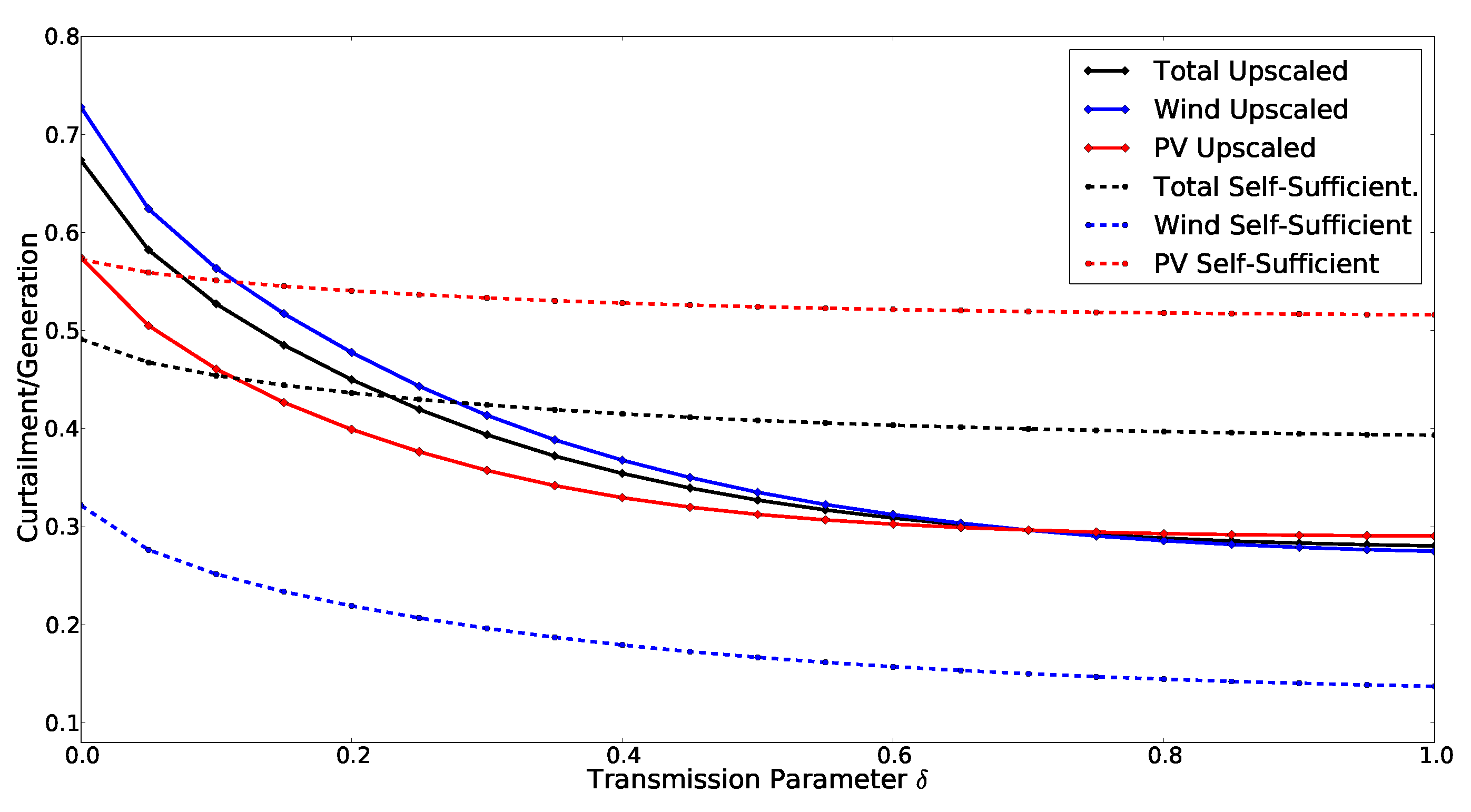
5.3. Limited Transmission

A major obstacle and the subject of intense political controversy is the reinforcement of the transmission grid. All previous results were calculated for unlimited transmission. In this section, it is investigated how curtailment changes if transmission capacities are reduced in an abstract way. First, transmission capacities for every link ${\kappa }_l$ are computed by the definitions in Equation (18). These transmission capacities are then all varied with a grid strength parameter $\delta \in [0,1]$ according to:

$${\kappa }_l^{\prime }=\delta {\kappa }_l^C$$

(26)

where $\delta =0$ means no transmission between nodes and $\delta =1$ means transmission capacities are sufficient to transfer all energy for every link 99% of the time. To investigate the impact of limited transmission on the curtailment, δ was varied between zero and one (Figure 9). For low transmission grid strength ($\delta <0.25$), curtailment is higher in the upscaled scenario compared to the self-sufficient scenario. For $\delta >0.25$, overall curtailment in the self-sufficient scenario exceeds the overall curtailment in the upscaled scenario. In general, transmission is more important in the upscaled scenario, i.e., total curtailment is reduced from 67% (no transmission) to 28% for $\delta =1.0$. For wind and PV considered separately, the reduction is similar: from 73% to 27% and from 57% to 29%, respectively. It also can be observed that for low transmission capacities, the curtailment of PV power is less than the curtailment of wind power, but this changes, if transmission capacities are increased. Therefore, it can be concluded that wind power benefits more from a strong transmission grid than PV does. For the self-sufficient scenario, almost no benefit from transmission for PV power, being the dominant source of generation, is noticeable. Wind contributes a smaller share of generation in this scenario, and the curtailment of wind energy can be reduced by strengthening transmission from 32% to 14%. The overall curtailment can be reduced in the self-sufficient scenario from 49% to 39%.

Figure 10 shows the effective capacity factors for $\delta =0.2$. Limiting the transmission capacities to 20% of the maximum transmission capacities decreases effective capacity factors for PV in counties far from the load centers (coastal regions, in Lower Bavaria and southern Brandenburg) by up to 50% in the upscaled scenario. In heavily-populated regions, like North Rhine-Westphalia or southern Lower Saxony, no effect is observed. In the self-sufficient case, almost no differences occur for most German counties. However, some counties see a further reduction of their effective capacity factors by ca. 15%. Limiting transmission hampers the export of the high surpluses and leads to high curtailment rates. The effect of limited transmission is stronger on wind than on PV (Figure 10, top). For the self-sufficient scenario, effective capacity factors in northern Germany decrease significantly, while in most other regions, no significant reduction occurs. In this case, most counties have very similar effective capacity factors for wind in the range of 10% to 14%, and the strong north-south gradient disappears. For the upscaled scenario, the transmission limitation has the most prominent (negative) effects, especially on the northern and eastern German regions. In fact, limiting transmission renders them the least favorable for wind power installations in Germany. This is a crucial result, as today, the wind power deployment is still strongest in these regions [41]. In a 100% renewable German power system with an inappropriate transmission grid, these wind power plants would not be economical any longer, because their capacity factor would be partly only 2%, because their surpluses cannot be exported in times of overall generation surpluses. In fact, the surpluses in the north are also the major cause for increased transmission capacity needs in the upscaled scenario (see Table 1).

6. Summary and Conclusions

Curtailment is the reduction in the output of a generator not induced by the non-availability of resources. With increasing renewable shares, the curtailed amount of energy consequently grows. Therefore, considering curtailment will be of increasing importance in the future. In this paper, the curtailment for 402 German counties that are all fully connected to their neighboring counties was investigated. Today, the common capacity factor is primarily considered for the site assessment of renewable power plants, because revenue generated by a power plant is linearly linked to its generated energy. In power systems with high shares of renewables, an effective capacity factor seems to be more appropriate to compare different sites with respect to their quality for renewable power deployment. For this investigation, an effective capacity factor was defined. It differs from the common capacity factor by considering only generation that is not curtailed. It was shown that several aspects influence curtailment and hence effective capacity factors. Two renewable scenarios have been defined for the distribution of capacities. In the upscaled scenario, today’s spatial capacity distribution within Germany is preserved, and the capacity of each generation facility was multiplied by a constant factor to meet demand. This scenario requires strong grid reinforcement to dampen curtailment as much as possible. In the self-sufficient scenario, every county was autarkic in the way that its average production meets its average consumption. This scenario is advantageous if the transmission grid is not very well developed. It only requires approximately 50% of the transmission capacity of the upscaled scenario to distribute all useable energy surpluses.

The share between wind and photovoltaics in a county and the whole country indirectly influences the curtailment and the overall need for transmission. This is caused by the strong correlation of wind and PV generation between different counties. If a county has a high wind share while the overall share of wind is low, this county experiences several export opportunities, when PV generation is low.

The effect of transmission limitations on effective capacity factors is complex. For PV transmission capacity reductions lead only to a small decrease in most regions. For wind, the effect is much stronger. For some regions, especially in eastern Germany and the coastal areas, effective capacity factors are lower than in central German regions, although meteorological capacity factors behave vice versa, if the transmission grid strength is significantly reduced. The importance of the transmission grid was investigated by reducing the transmission capacity between every pair of nodes to a fraction of the maximum required to transmit all surplus energies. In both scenarios, it was demonstrated that transmission has the potential to reduce curtailment of wind power by two thirds. The benefit for PV by increased transmission is smaller. In the self-sufficient scenario, no significant reduction of curtailment for PV power by increased transmission capacities was observed. In the upscaled scenario, the maximum reduction of curtailment for PV by transmission is ca. 50%. Future work should investigate the interplay of storage and curtailment, power exports/imports to/from neighboring countries and the role of German offshore wind power.

References

- Burger, B. Electricity Production from Solar and Wind in Germany in 2014; Fraunhofer ISE: Freiburg, Germany, 2013. [Google Scholar]
- Jacobson, M.Z.; Delucchi, M.A. Providing all global energy with wind, water, and solar power, Part I: Technologies, energy resources, quantities and areas of infrastructure, and materials. Energy Policy 2011, 3, 1154–1169. [Google Scholar] [CrossRef]
- De Vries, B.J.; van Vuuren, D.P.; Hoogwijk, M.M. Renewable energy sources: Their global potential for the first-half of the 21st century at a global level: An integrated approach. Energy Policy 2007, 35, 2590–2610. [Google Scholar] [CrossRef]
- Hasche, B. General statistics of geographically dispersed wind power. Wind Energy 2010, 13, 773–784. [Google Scholar] [CrossRef]
- Wiemken, E.; Beyer, H.; Heydenreich, W.; Kiefer, K. Power characteristics of PV ensembles: Experiences from the combined power production of 100 grid connected PV systems distributed over the area of Germany. Sol. Energy 2001, 70, 513–518. [Google Scholar] [CrossRef]
- Boccard, N. Capacity factor of wind power realized values vs. estimates. Energy Policy 2009, 37, 2679–2688. [Google Scholar] [CrossRef]
- Abed, K.A.; El-Mallah, A.A. Capacity factor of wind turbines. Energy 1997, 22, 487–491. [Google Scholar] [CrossRef]
- Justus, C.; Hargraves, W.; Yalcin, A. Nationwide assessment of potential output from wind-powered generators. J. Appl. Meteorol. 1976, 15, 673–678. [Google Scholar] [CrossRef]
- Diakov, V. Wind resource quality affected by high levels of renewables. Resources 2015, 4, 378–383. [Google Scholar] [CrossRef]
- Gu, Y.; Xie, L.; Rollow, B.; Hesselbaek, B. Congestion-induced wind curtailment: Sensitivity analysis and case studies. In Proceedings of the North American Power Symposium (NAPS), Boston, MA, USA, 4–6 August 2011; IEEE: Boston, MA, USA, 2011; pp. 1–7. [Google Scholar]
- Flora, R.; Marques, A.C.; Fuinhas, J.A. Wind power idle capacity in a panel of European countries. Energy 2014, 66, 823–830. [Google Scholar] [CrossRef]
- Faulstich, M.; Foth, H.; Calliess, C.; Hohmeyer, O.; Holm-Mueller, K.; Niekisch, M.; Schreurs, M. Climate-friendly, Reliable, Affordable: 100% Renewable Electricity Supply by 2050; Technical Report; German Advisory Council on the Environment (SRU): Berlin, Germany, 2010. [Google Scholar]
- Bundesnetzagentur. EEG in Zahlen. 2015. Available online: http://www.bundesnetzagentur.de/cln1422/DE/Sachgebiete/ElektrizitaetundGas/UnternehmenInstitutionen/ErneuerbareEnergien/ZahlenDatenInformationen/zahlenunddaten-node.html (accessed on 3 October 2015).
- Lew, D.; Bird, L.; Milligan, M.; Speer, B.; Wang, X.; Carlini, E.M.; Estanqueiro, A.; Flynn, D.; Gomez-Lazaro, E.; Menemenlis, N.; et al. Wind and solar curtailment. In Proceedings of the 12th International Workshop on Large-Scale Integration of Wind Power into Power Systems as well as on Transmission Networks for Offshore Wind Power Plants, London, UK, 22–24 October 2013.
- EirGrid; SONI. Delivering a Secure Sustainable Electricity System; Project Presentation; EirGrid: Dublin, Ireland, 2013. [Google Scholar]
- Bundesamt für Kartographie und Geodäsie. 2015. Available online: http://www.bkg.bund.de (accessed on 31 July 2015).
- Statistische Ämter des Bundes und der Länder. 2015. Available online: http://www.regionalstatistik.de (accessed on 31 July 2015).
- Negra, N.B.; Todorovic, J.; Ackermann, T. Loss evaluation of HVAC and HVDC transmission solutions for large offshore wind farms. Electr. Power Syst. Res. 2006, 76, 916–927. [Google Scholar] [CrossRef]
- Heide, D.; von Bremen, L.; Greiner, M.; Hoffmann, C.; Speckmann, M.; Bofinger, S. Seasonal optimal mix of wind and solar power in a future, highly renewable Europe. Renew. Energy 2010, 35, 2483–2489. [Google Scholar] [CrossRef]
- Kies, A.; Nag, K.; von Bremen, L.; Lorenz, E.; Heinemann, D. Investigation of balancing effects in long term renewable energy feed-in with respect to the transmission grid. Adv. Sci. Res. 2015, 12, 91–95. [Google Scholar] [CrossRef]
- Oswald, B.; Oeding, D. Elektrische Kraftwerke und Netze, 6th ed.; Springer-Verlag: Berlin/Heidelberg, Germany; New York, NY, USA, 2004. [Google Scholar]
- Heide, D. Statistical Physics of Power Flows on Networks with a High Share of Fluctuating Renewable Generation. Ph.D. Thesis, Johann Wolfgang Goethe-Universitaet Frankfurt am Main, Frankfurt, Germany, 2010. [Google Scholar]
- Rodriguez, R.A.; Dahl, M.; Becker, S.; Greiner, M. Localized vs. synchronized exports across a highly renewable pan-European transmission network. Energy Sustain. Soc. 2015, 5, 1–9. [Google Scholar] [CrossRef]
- Heide, D.; Greiner, M.; von Bremen, L.; Hoffmann, C. Reduced storage and balancing needs in a fully renewable European power system with excess wind and solar power generation. Renew. Energy 2011, 36, 2515–2523. [Google Scholar] [CrossRef]
- Rodriguez, R.A.; Becker, S.; Greiner, M. Cost-optimal design of a simplified, highly renewable pan-European electricity system. Energy 2015, 83, 658–668. [Google Scholar] [CrossRef]
- Kies, A.; von Bremen, L.; Chattopadhyay, K.; Lorenz, E.; Heinemann, D. Backup, storage and transmission estimates of a supra-European electricity grid with high shares of renewables. In Proceedings of the 14th Wind Integration Workshop, Brussels, Belgium, 20–22 October 2015.
- Becker, S.; Rodriguez, R.; Andresen, G.; Schramm, S.; Greiner, M. Transmission grid extensions during the build-up of a fully renewable pan-european electricity supply. Energy 2014, 64, 404–418. [Google Scholar] [CrossRef]
- Becker, S.; Frew, B.A.; Andresen, G.B.; Zeyer, T.; Schramm, S.; Greiner, M.; Jacobson, M.Z. Features of a fully renewable US electricity system: Optimized mixes of wind and solar PV and transmission grid extensions. Energy 2014, 72, 443–458. [Google Scholar] [CrossRef]
- Rodriguez, R.A.; Becker, S.; Andresen, G.B.; Heide, D.; Greiner, M. Transmission needs across a fully renewable European power system. Renew. Energy 2014, 63, 467–476. [Google Scholar] [CrossRef]
- Doms, G.; Schättler, U.; Baldauf, M. A Description of the Nonhydrostatic Regional COSMO Model, Part I: Dynamics and Numerics; Technical Report; Consortium for Small-Scale Modelling: Offenbach, Germany, 2011. [Google Scholar]
- Späth, S.; von Bremen, L.; Junk, C.; Heinemann, D. Time-consistent calibration of short-term regional wind power ensemble forecasts. Meteorol. Z. 2015, 24, 381–392. [Google Scholar]
- Klucher, T. Evaluation of models to predict insolation on tilted surfaces. Sol. Energy 1979, 23, 111–114. [Google Scholar] [CrossRef]
- SMA Solar Technology AG. Sunny Mini Central 6000TL/7000TL/8000TL; SMA Solar Technology AG: Niestetal, Germany, 2010. [Google Scholar]
- Bundesministerium für Wirtschaft und Energie. Erneuerbare Energien in Zahlen—Nationale und Internationale Entwicklung im Jahr 2013; Bundesministerium für Wirtschaft und Energie: Berlin, Germany, 2014. [Google Scholar]
- Grimm, V.; Martin, A.; Weibenzahl, M.; Zoettl, G. Transmission and generation investment in electricity markets: The effects of market splitting and network fee regimes. Eur. J. Oper. Res. 2016, 254, 493–509. [Google Scholar] [CrossRef]
- Kemfert, C.; Kunz, F.; Rosellón, J. A Welfare Analysis of the Electricity Transmission Regulatory Regime in Germany. DIW: Berlin, Germany, 2015. [Google Scholar]
- Baringo, L.; Conejo, A.J. Transmission and wind power investment. IEEE Trans. Power Syst. 2012, 27, 885–893. [Google Scholar] [CrossRef]
- Orfanos, G.A.; Georgilakis, P.S.; Hatziargyriou, N.D. Transmission expansion planning of systems with increasing wind power integration. IEEE Trans. Power Syst. 2013, 28, 1355–1362. [Google Scholar] [CrossRef]
- Erneuerbare-Energien-Gesetz, 2014. Available online: http://dejure.org/gesetze/EEG/12.html (accessed on 15 March 2016).
- Deutschlands Zukunft Gestalten—Koalitionsvertrag Zwischen CDU, CSU und SPD, 2013. Available online: http://www.bundesregierung.de/Content/DE/Anlagen/2013/2013-12-17-koalitionsvertrag.pdf (accessed on 18 March 2016).
- Betreiberdatenbasis: Betriebsdaten von Windanlagen. Available online: http://www.btrdb.de/ (accessed on 10 January 2015).