1. Introduction
There has been a global interest in renewable energy resources due to the worldwide increase in power demand and the limitation of fossil fuels and their harmful impact on the environment. Renewable energy resources, such as wind energy, are naturally available, clean and have a much less harmful impact on the environment than fossil fuels.
Wind energy is the fastest growing renewable energy resource. Globally, the annual cumulative installed wind energy capacity has increased rapidly during the period from 1997–2014 [
1]. In addition, the advancement on the design of the components of wind energy power systems that include power electronics inverters, electric generators and drive train systems has also contributed to the fast growth and high demand of wind energy conversion systems (WECs). The increasing market share of variable speed wind energy conversion systems has led to further investigations of wind turbines’ control technology. Furthermore, researchers have recognized that appropriate control algorithms can greatly improve the efficiency of wind power conversion systems.
Among the various types of available wind turbines, the doubly-fed induction generator-based wind turbines are widely used for variable speed wind turbine systems because of their simple structures, their reliable operations, their high power densities and their energy efficiency. Moreover, doubly-fed induction generators-based energy systems have other advantages, such as the reduction of mechanical stress, the flexibility in controlling active and reactive powers and the ability to track maximum power using different control techniques.
Many research articles dealing with the design of different types of control schemes for DFIG-based variable speed wind turbine systems were published in the last few years; for example, the reader can refer to the works in [
2,
3,
4,
5,
6,
7,
8,
9,
10,
11,
12,
13,
14,
15,
16] for a detailed review of wind turbine systems and their control. Some of these control techniques are highlighted below.
Researchers have used different control techniques to control DFIG-based wind turbine energy systems. For example, PID controllers and several modified PID control schemes were used to control wind energy conversion systems [
17,
18,
19]. These types of schemes are believed to be the easiest and simplest design methods. However, DFIG-based wind energy systems are highly nonlinear systems, which are characterized by strong couplings between the different variables of the systems. Thus, nonlinear control schemes need to be designed to control wind energy power systems so that the desired performances are attained.
The work in [
20] proposed a method for obtaining the maximum power output of a DFIG-based wind energy system. The proposed control technique was based on the usage of an improved maximum power point tracking (MPPT) curve method and a Lyapunov function. In [
21], an artificial neural network technique based on Markov scheme approaches was developed to optimize the output of a wind turbine system. An artificial neural network, which is based on the Jordan re-current concept, was used to estimate the reference tracking speed of the rotor in [
22]. A direct and an indirect control structure using a quantum neural network to enhance the efficiency of the system and to optimize the output of a wind energy power system was proposed in [
23]. Furthermore, the combination of fuzzy logic control and sliding mode control was investigated in the literature; for example, refer to the works in [
24,
25,
26,
27,
28].
Investigations to determine the best nonlinear control technique that can be used to improve the performance of DFIG-based WEC systems are still ongoing [
29]. The control of both the grid side converter (GSC) and the rotor side converter (RCS) in one control loop was reported in [
30]. In [
31], a direct active power and reactive power controller based on the estimation of the stator flux was proposed, and a basic hysteresis controller was used. Vector control and direct power control were proposed in [
32] to regulate the active power and reactive power generated by a DFIG-based wind energy system. In [
33], two distinct control strategies were used to control a DFIG-based WEC system; backstepping and sliding mode control strategies were first used to control the rotor side converter (RCS); then, the same strategies were used to control the grid side converter (GSC). A perturbation observer-based control scheme for the control of DFIG in a multi-machine power system was introduced in [
34]. The controller is achieved with a four-loop perturbation observer-based control configuration, and the controlled dynamics were investigated through simulation studies.
Several researchers investigated the usage of the feedback linearization technique for the control of DFIG-based WEC systems. Some of these works are highlighted below. An input-output feedback linearization controller for a DFIG-based system connected to an infinite bus was discussed in [
35]; the authors differentiated the electromagnetic torque, the stator power and the grid side converter power outputs of the DFIG to obtain a linear relationship with the rotor voltages, which serve as control inputs. Then, decoupled torque control and decoupled power control were developed. In [
36], an input-output linearizing and decoupling control strategy was proposed for a doubly-fed induction generator system. The developed controller was verified by using a 7.5 kW wind power test rig. A mathematical model of the DFIG based on the so-called stator magnetizing current field orientation was given in [
37]; then, an input-output linearizing controller is proposed. The controller results in decoupled control and the tracking of the generated active and reactive powers of the system. Direct control of the torque and direct control of the power outputs of the DFIG were established based on the input-output feedback linearization technique in [
38,
39]. In [
40], an adaptive nonlinear control strategy based on a feedback linearization scheme was proposed for a DFIG-based WEC system; a disturbance observer was added to estimate the uncertainties in the parameters of the system. The performance of the system is checked in the presence of nearby faults. Moreover, an exact feedback linearization scheme was proposed in [
41] for a DFIG-based WEC system. The wind turbine with DFIG is represented by a third-order model. This model is exactly linearized, and a linear quadratic regulator is used to design an optimal controller for the linearized system. Simulations were performed on a single machine infinite bus system and on a four-machine system; the simulation results indicate that the proposed control scheme improves the transient stability of the power system, and it enhances the damping of the system.
The contribution of this paper involves the design of an input-state feedback linearization controller for a wind energy conversion system. Previous works on feedback linearization of WEC systems, generally, used fifth order models or sixth order models. Our work uses an eighth order model of the WEC system; the state space representation of the eighth order model under consideration uses four electrical states and four mechanical states. The proposed controller controls the rotor side converter (RCS) of a DFIG. It guarantees the stability of the closed loop system and enables the tracking of the desired states of the system. In addition, the proposed controller maximizes the power extracted from the wind. The proposed theoretical work is verified through MATLAB simulations; moreover, the validity of the proposed controller was tested when some of the parameters of the system change.
The rest of the paper is organized as follows.
Section 2 presents the model of a DFIG-based wind energy power system; the system consists of eight nonlinear ordinary differential equations. In
Section 3, the computations of the values of the desired states of the system, as well as the reference inputs are discussed in detail.
Section 4 presents the design of an input-state feedback linearization controller for the wind energy conversion system. To show the effectiveness of the proposed controller, simulation studies are presented in
Section 5. In addition, some simulation results are shown to investigate the robustness of the controller to changes in some of the parameters of the system. Finally, the conclusion is drawn in
Section 6.
2. Model of the Wind Energy Conversion System
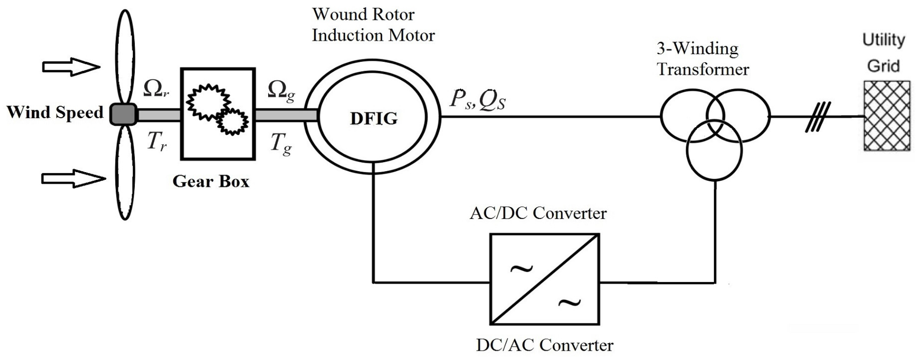
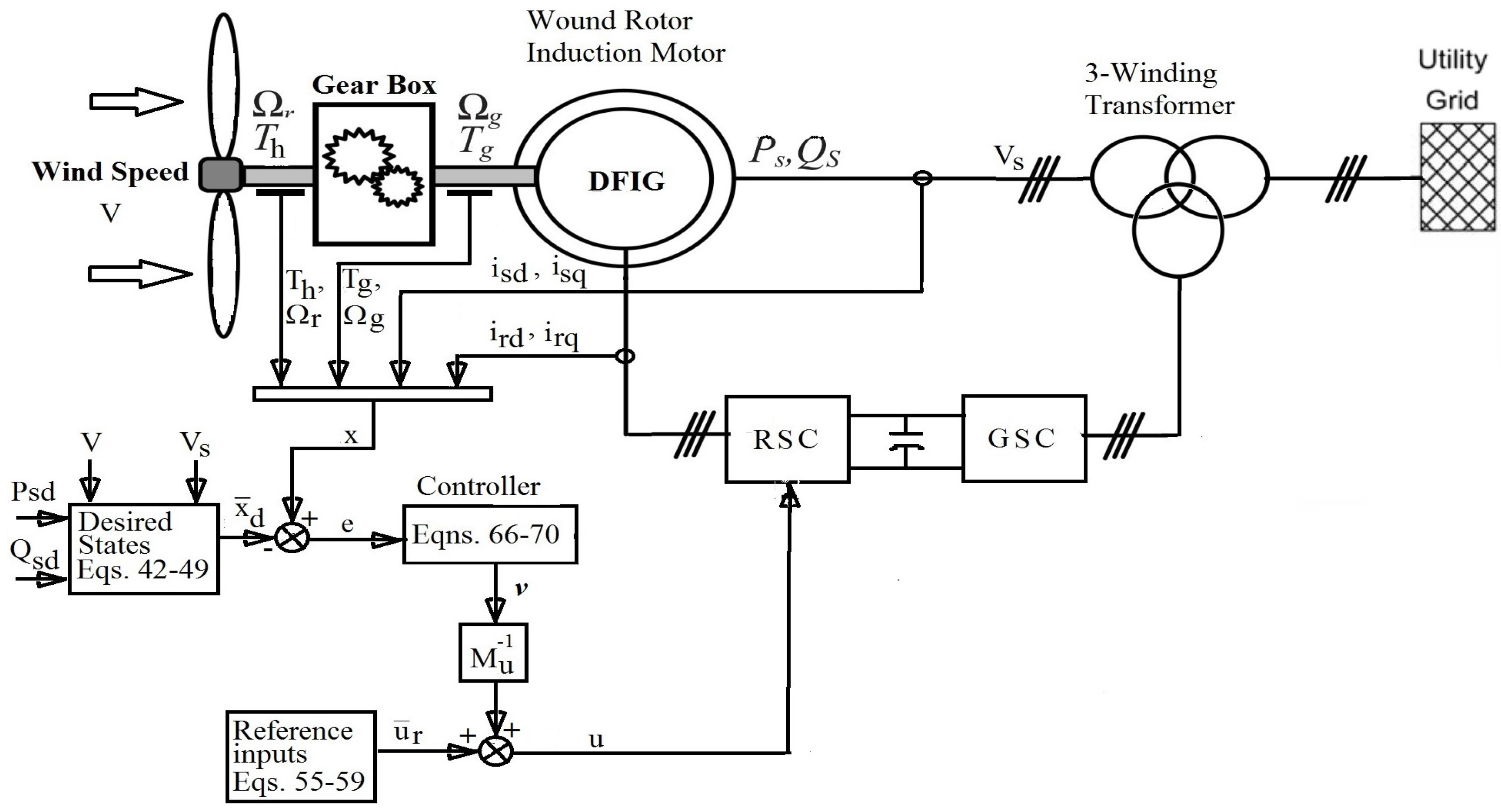
The model of a DFIG-based wind energy conversion power system is presented in this section. A block diagram depiction of the system is shown in
Figure 1. The system consists of a wind turbine connected through a gear box to a doubly-fed induction generator. The stator windings of the standard wound induction generator are directly connected to the grid. The rotor windings are connected to the grid through a voltage source and power electronics converters (AC/DC/AC). The wind energy is captured by the motor blades and transferred to the motor hub. The hub has a gearbox, which attaches the low-speed shaft to the high-speed shaft that drives the DFIG, which converts the mechanical energy to electrical energy. This electrical energy is delivered to the grid.
Note that
,
,
and
depicted in
Figure 1 represent the rotational speed of the turbine on the low-speed side of the gearbox, the mechanical speed of the generator, the high-speed shaft torque and the generator torque, respectively. Furthermore
and
are the stator active power and the stator reactive power.
The mechanical power extracted from the wind can be expressed as [
42],
where:
: the captured wind power (the mechanical power),
: the power coefficient,
λ: the tip speed ratio ,
β: the pitch angle,
ρ: the air density,
R: the rotor-plane radius,
V: the speed of the wind.
The tip speed ratio can be expressed as,
where
is the rotational speed of the turbine on the low-speed side of the gearbox.
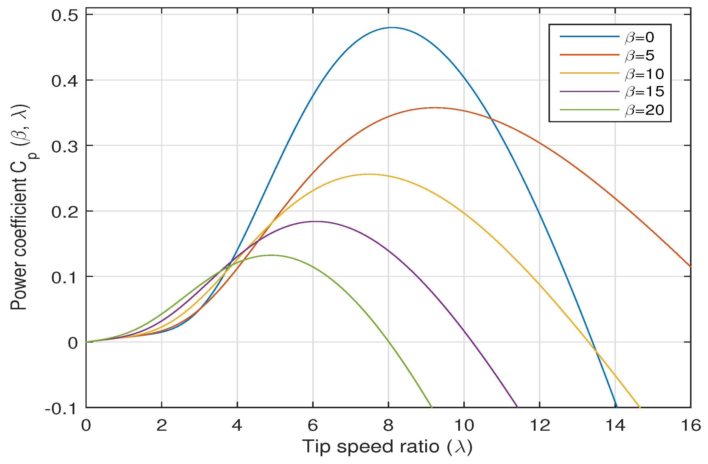
The power coefficient
versus the tip speed ratio
λ for different values of the pitch angle
β is depicted in
Figure 2. It can be seen from the figure that when
, the maximum value of
is achieved when
at an optimal value of the tip speed ratio
. To capture the maximum power from the wind, a variable speed wind turbine normally follows the
up to the rated speed by varying the rotor speed to keep the tip speed ratio at its optimum value
.
Using Equation (1), the maximum captured wind power,
, can be written as,
The aerodynamic torque,
, can be expressed as follows,
The wind turbine varies its speed by following the maximum value of the power coefficient
so that maximum power is captured. This is done by changing the speed of the rotor to maintain the tip speed ratio at its optimum value
[
42]. Using Equations (2)–(4), the aerodynamic torque,
, can be written as follows,
where
.
To model the wind energy power system, we first need to define the state variables of the system. The system consists of an electrical part and a mechanical part. The state variables of the electrical part of the system are the stator currents in the d and q axes ( and ) and the rotor currents in the d and q axes ( and ). The state variables of the mechanical part of the system are the rotational speed of the turbine on the low-speed side of the gearbox (), the mechanical speed of the generator (), the high-speed shaft torque () and the generator torque (). The inputs for the system are the stator and rotor voltages and the required generator torque (). Note that the voltage is the d-axis stator voltage, and is the q-axis stator voltage. The voltage is the d-axis rotor voltage, and is the q-axis rotor voltage.
The rotational speed of the generator
is related to the rotor angular frequency
, such that,
where
is the number of pole pairs of the generator.
The stator angular frequency
is related to the stator frequency,
, such that,
Furthermore, the leakage coefficient can be written, such that,
where
is the magnetizing inductance,
is the rotor leakage inductance and
is the stator leakage inductance.
The model of the wind energy power system consists of eight first order ordinary differential equations (odes). The first four odes are related to the electrical part of the system; the second four odes are related to the mechanical part of the system. Hence, the wind turbine energy conversion system can be described using the following set of nonlinear ordinary differential equations, such that [
42,
43],
where:
: the damping constants for the generator,
: the damping constants for the the equivalent low-speed shaft,
: the damping constants for the rotor,
: the magnetizing current,
: the moment of inertia of the generator,
: the moment of inertia of the rotor,
: the equivalent torsional stiffness of the low-speed shaft,
: the gearbox ratio (the gearbox is considered as a lossless device for this model),
: the rotor resistance,
: the stator resistance,
: the time constant of the model,
: the stator voltage magnitude.
For the ease of presentation, we define the following parameters for the wind energy conversion system, , , , , , , , , , , , , , , , , , , , , , , .
Moreover, we define the state variable vector
x, which contains the states
–
, such that,
Therefore, the model of the wind energy power system in (10) can be written in compact form as follows,
Let the desired state vector
be such that
, where
are the desired values of the states
of the power system. Since the desired states have to be an operating point of the power system, then they must satisfy the equations of the model of the wind energy power system in (12). Therefore, the desired states of the power system are governed by the following set of differential equations:
Note that , , , and in (12)–(19) represent the reference inputs of the wind energy conversion system. The computation of these reference inputs will be discussed in the next section.
Define the errors
, such that:
Using Equations (12)–(21), the dynamic model of the error system can be written, such that:
where the inputs
,
,
,
and
are defined, such that,
After some manipulations, the error dynamics in (22) can be written as follows,
Define the matrix
and the vectors
u,
v and
, such that,
Remark 1. The controller of the wind energy conversion system model in (12) is computed using the controller and the reference inputs ,
,
,
and , such that,Equation (32) can be written in compact form, such that,Note that the determinant of the matrix equals , which is different from zero. Hence, the matrix is nonsingular, and its inverse always exists. 4. A Feedback Linearization Controller for the Wind Energy Conversion System
This section deals with the design of a feedback linearization control law for the wind energy conversion system represented by the nonlinear system of odes given by (12).
We start with defining the variables
,
and
, such that,
Furthermore, define the functions
and
, such that:
Let the control parameters , , and be positive scalars and choose the parameters , and to be positive scalars, such that the polynomial is Hurwitz.
The following proposition gives the feedback linearization controller.
Proposition 1. The feedback linearization controller,with and given by (31) and (55)–(59) and , such that,when applied to the model of the wind energy power system given by (12) guarantees the asymptotic convergence of the states of the system to their desired values. Note that the block diagram representation of the DFIG-based WEC system with the proposed controller is depicted in Figure 3. Proof. Applying the controllers given by (66)–(69) to the first four differential equations of the error system given by (23)–(26), we obtain:
Because the ’s are chosen to be positive scalars and since the parameters and are negative, then it can be concluded from the system of odes in (72) that the errors , , and asymptotically converge to zero as t tends to infinity.
The second part of the proof involves proving the asymptotic convergence to zero of the errors
,
,
and
. Taking the time derivative of the variables
and
defined in Equations (60)–(62) and using the equations of the error system given by (23)–(30), we obtain:
The application of the controller
in (70) to the system of odes in (73), yields,
The above system can be written in compact form, such that:
with the matrix
and the vector
z being such that,
Since , and are positive scalars, such that the polynomial is Hurwitz, then the matrix is a stable matrix (i.e., its eigenvalues are located in the left half of the s-plane). The solution of the Equation (74) is , where is the value of when . Therefore, the asymptotic convergence of , and to zero as t tends to infinity is guaranteed because is a stable matrix.
The zero dynamics [
44] is defined as the internal dynamics of the system when the output is kept identically zero by a suitable input function. For the third order system given by (73), the zero dynamics is analyzed by studying Equations (27)–(30) when
,
and
.
Using Equations (60) and (61), it is clear that the asymptotic convergence of and to zero implies the asymptotic convergence of and to zero as t tends to infinity.
Moreover, since
,
,
and
converge to zero as
t tends to infinity, then the equation given by (62) yields,
As
t tends to infinity, the differential Equation (28) of the error system given by (23)–(30), which represents the zero dynamics of the system, reduces to,
The constant
in (76) is such that,
Therefore, since is always negative, Equation (76) guarantees the asymptotic convergence of the error to zero as t tends to infinity. Moreover, Equation (75) implies the asymptotic convergence of the error to zero as t tends to infinity.
The asymptotic convergence to zero of the errors as t tends to infinity implies the asymptotic convergence of the states of the wind energy power system given by (12) to their desired values as t tends to infinity. ☐
5. Simulation Results of the Controlled Wind Energy Power System
The performance of the wind energy conversion system controlled using the proposed feedback linearization controller was simulated using the MATLAB software. The parameters of the system used for the simulation studies are given in
Table 1.
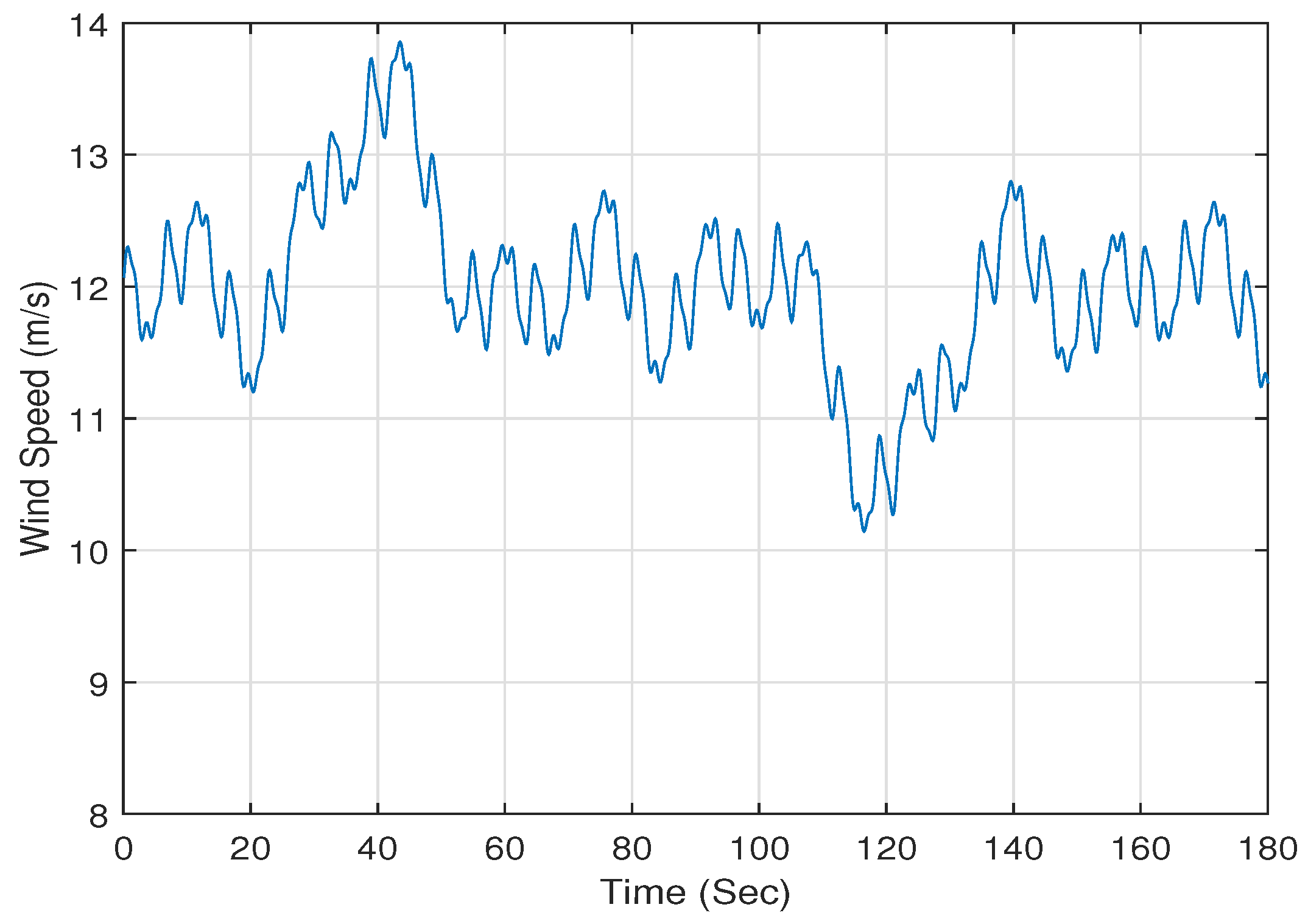
The wind speed model used for simulation purposes is given by the following formula:
with
. The wind speed profile versus time generated using Equation (78) is depicted in
Figure 4.
The wind energy conversion system was modeled using Equation (12) and controlled using the proposed feedback linearization control scheme given by Equations (65)–(70). The desired values of the states of the wind energy conversion system are obtained using Equations (42)–(49). The gains of the controller are taken to be: , , , , , and .
5.1. Simulation Studies of the WEC System When Using the Nominal Parameters of the System
The simulation results of the controlled system when using the nominal parameters are presented in
Figure 5,
Figure 6,
Figure 7,
Figure 8,
Figure 9,
Figure 10,
Figure 11,
Figure 12 and
Figure 13.
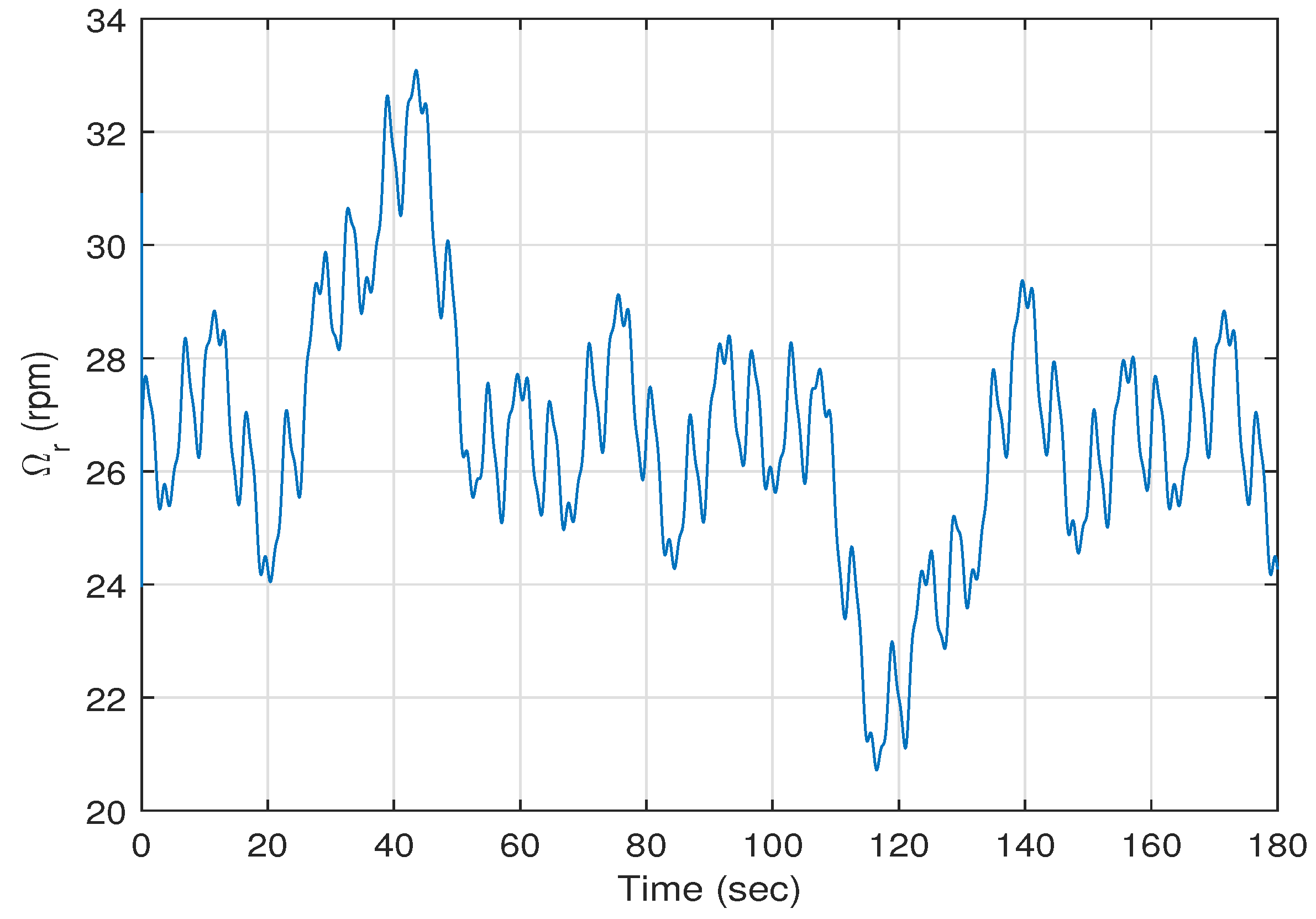
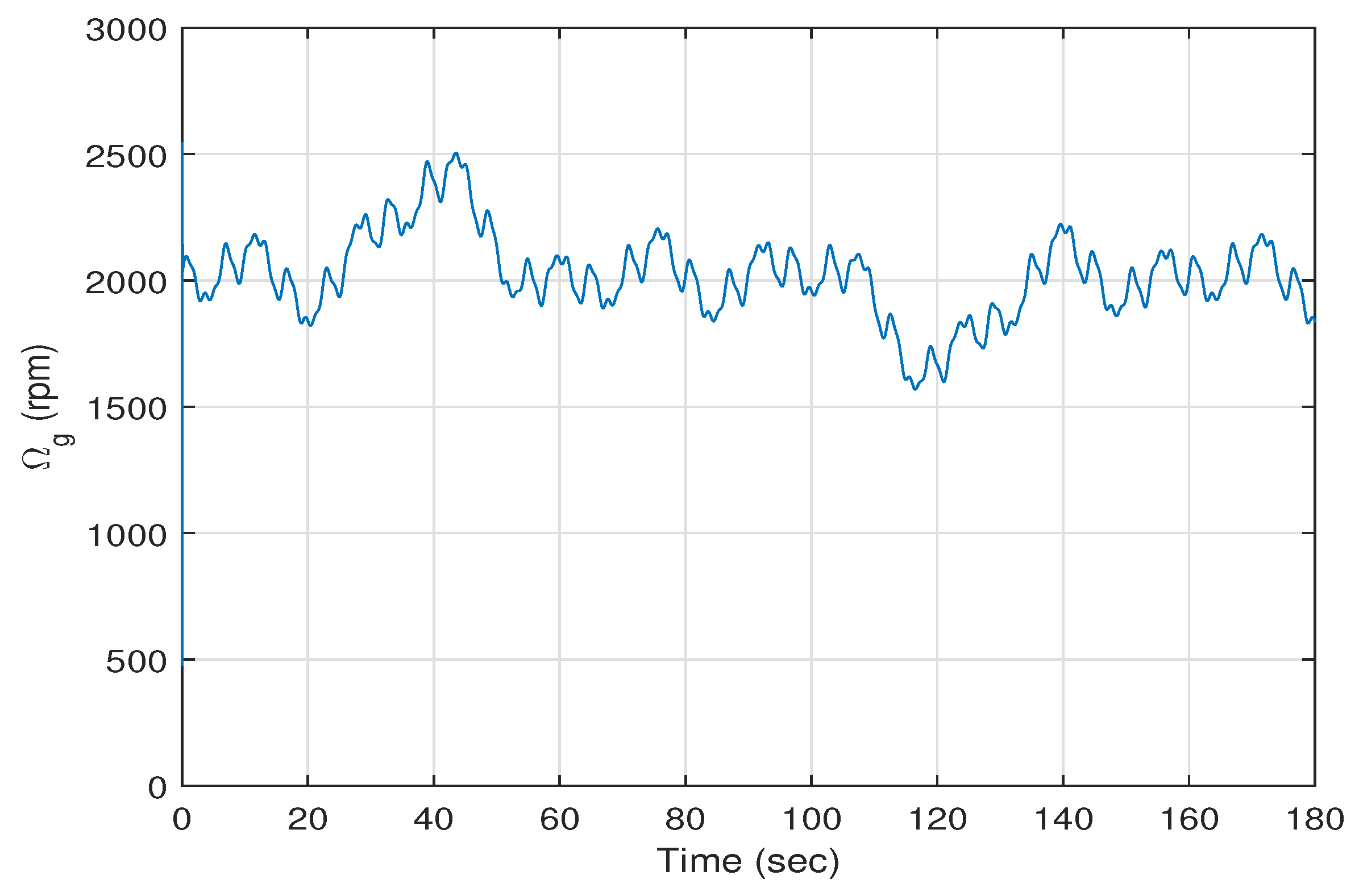
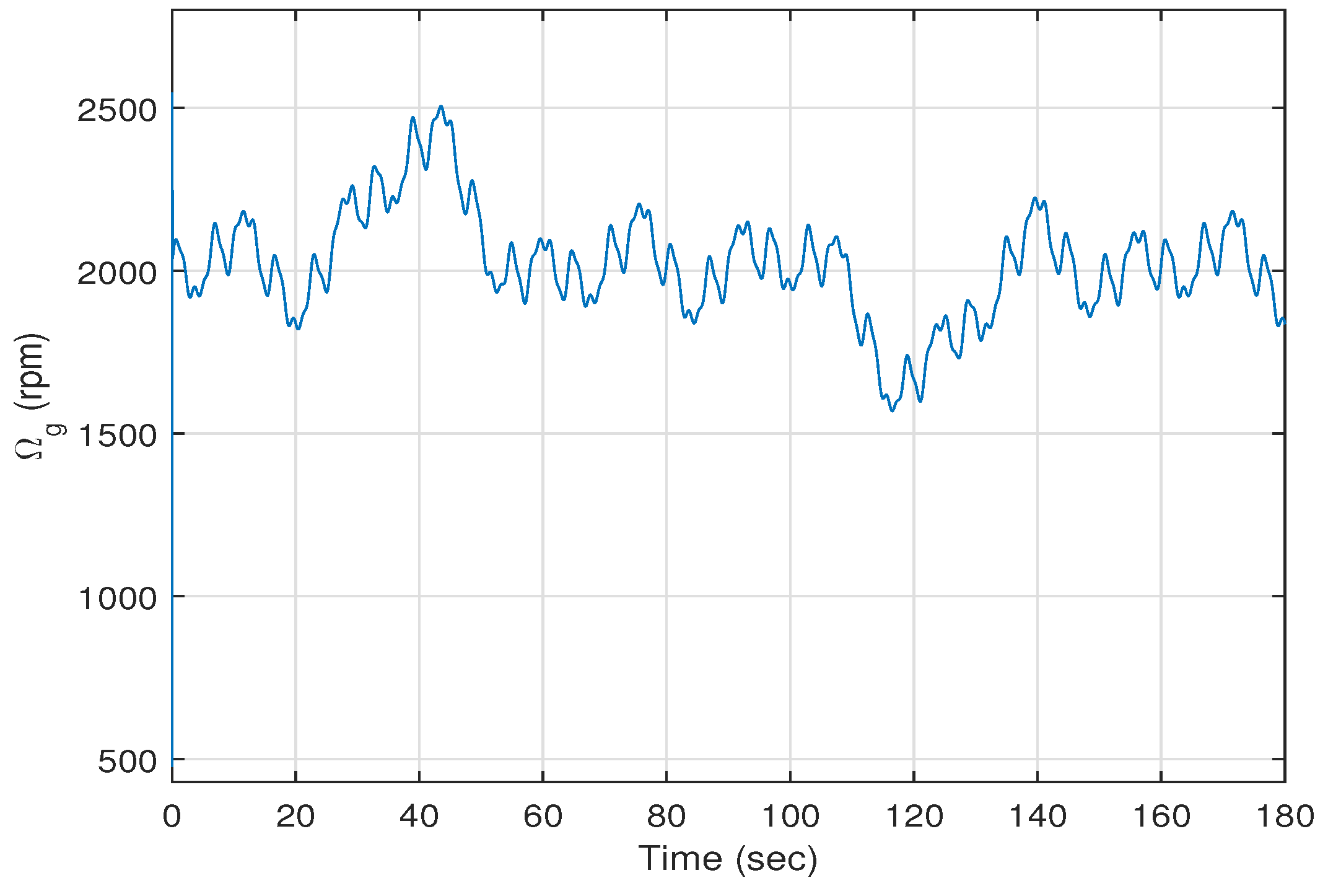
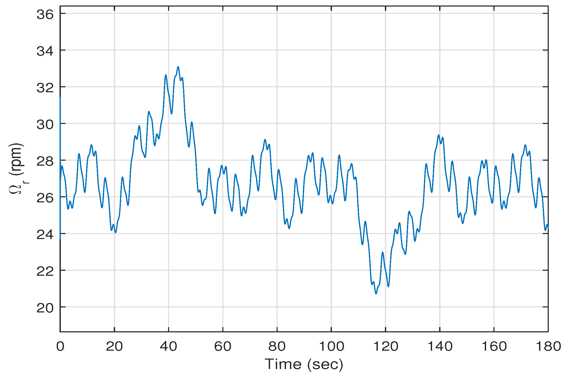
Figure 5 shows the trajectory of the rotor speed
versus time, and
Figure 6 depicts the trajectory of the generator speed
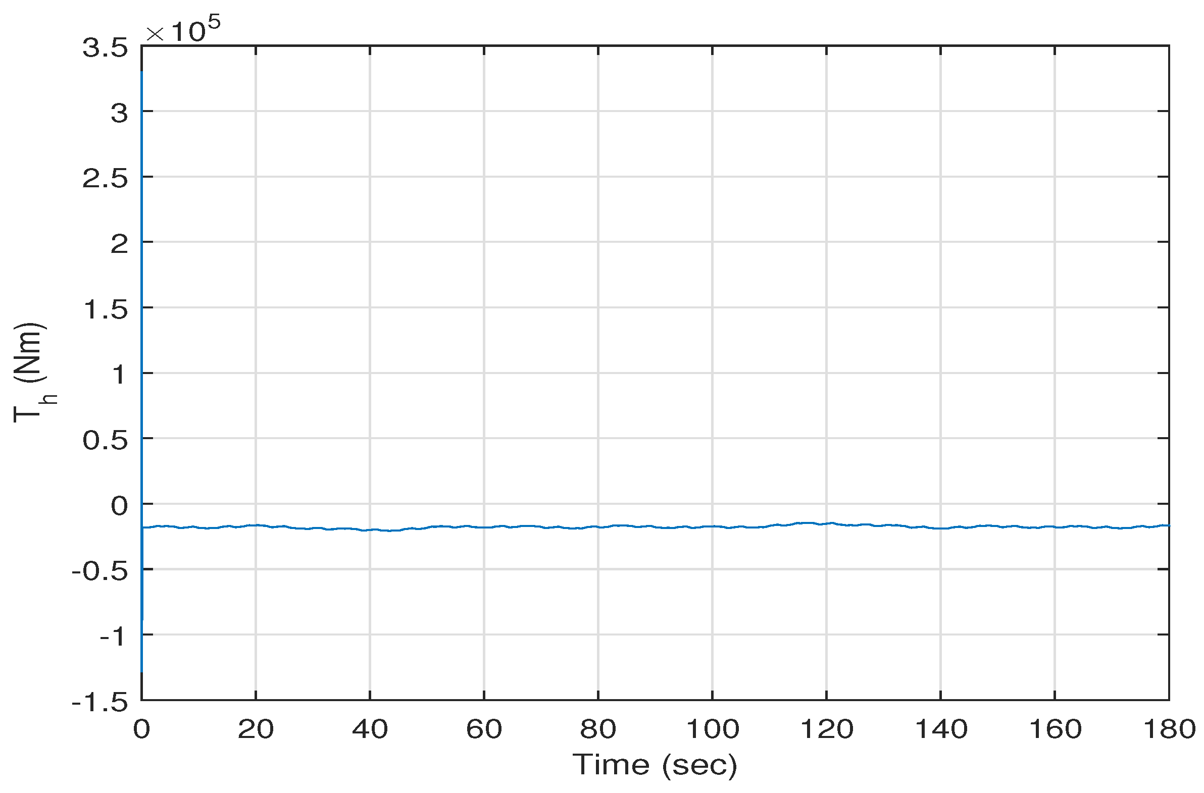
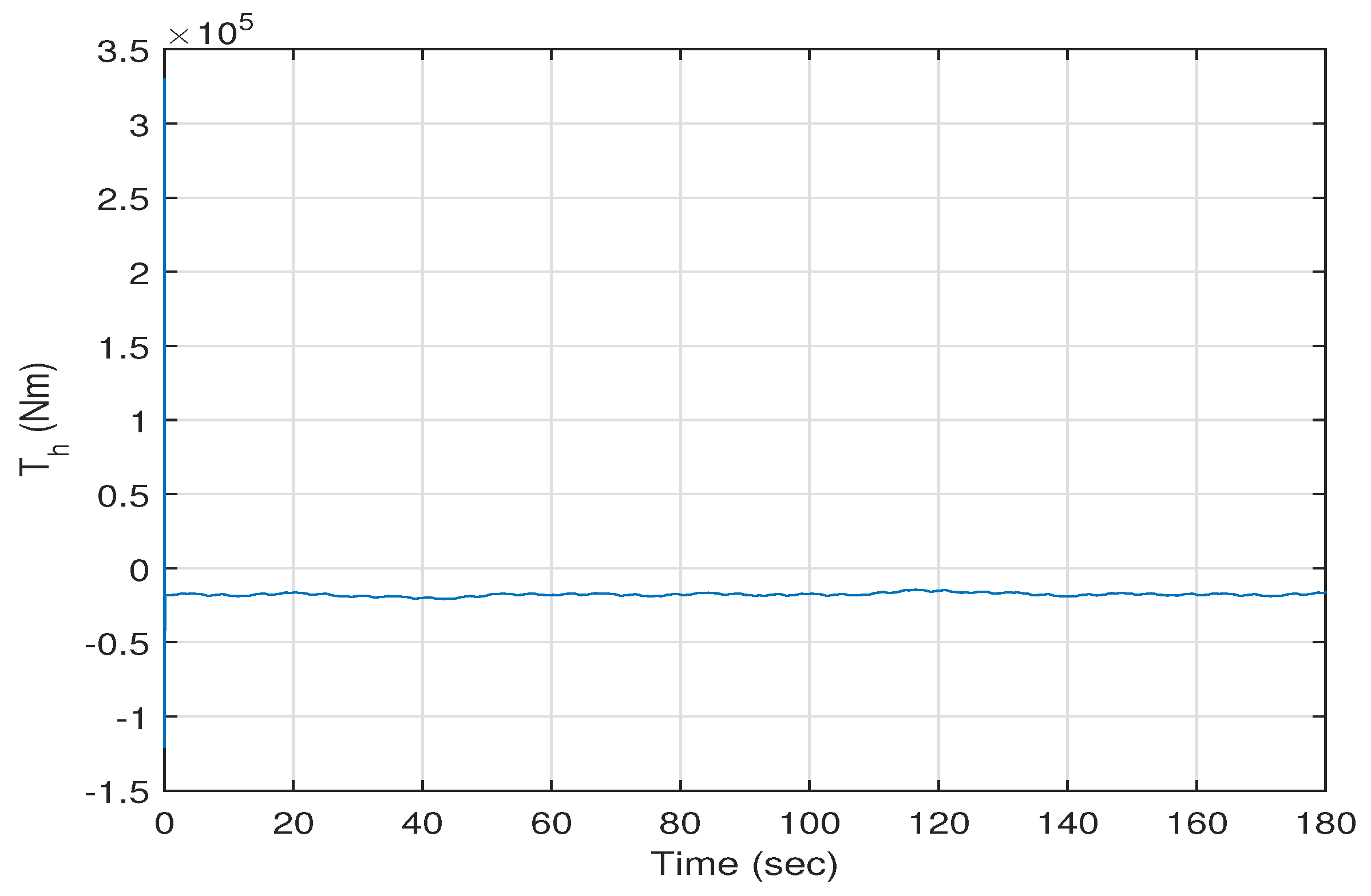
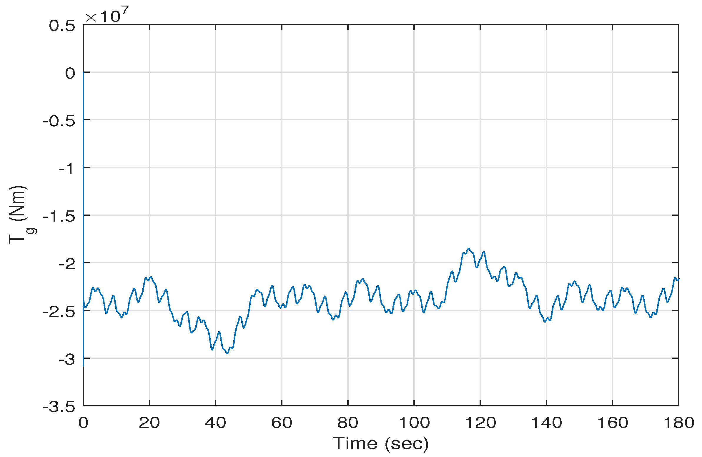
versus time. The high speed shaft torque and the generator torque versus time are shown in
Figure 7 and
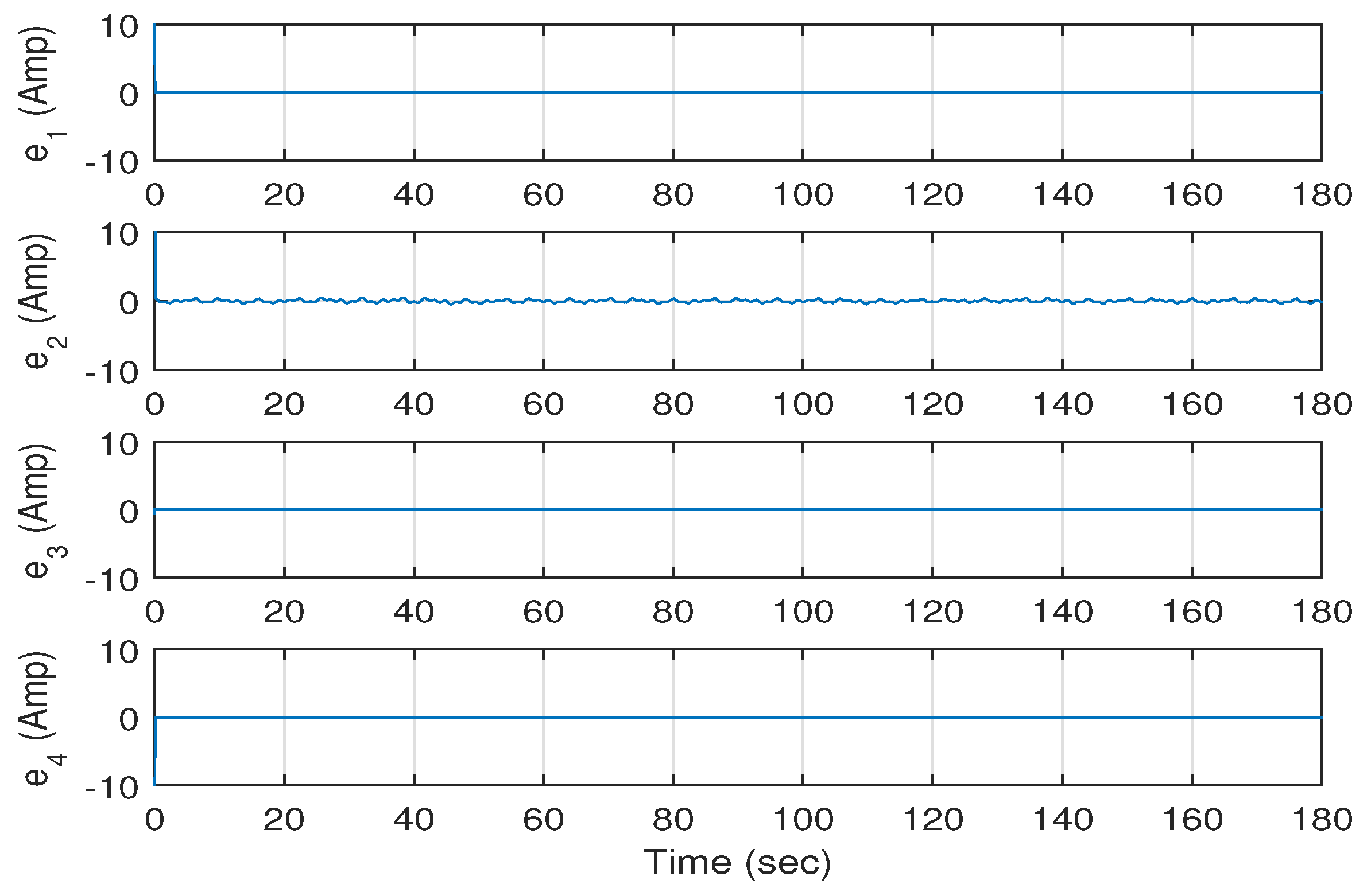
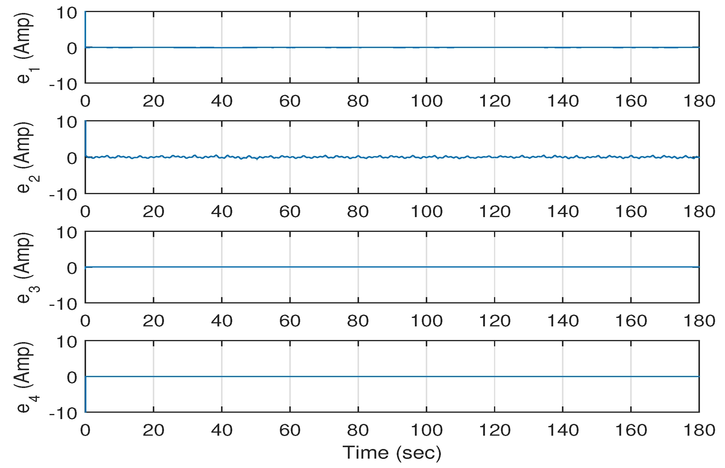
Figure 8. The errors between the actual and the desired values of the eight states of the system are shown in in
Figure 9 and
Figure 10.
Figure 9 shows the errors in the electrical state variables of the system versus time. It is clear from this figure that the errors
,
and
converge to zero. However, the error
shows some fluctuations around zero; these fluctuations are due to the fact that
, which is equal to
, where
is proportional to
(
V is the speed of the wind).
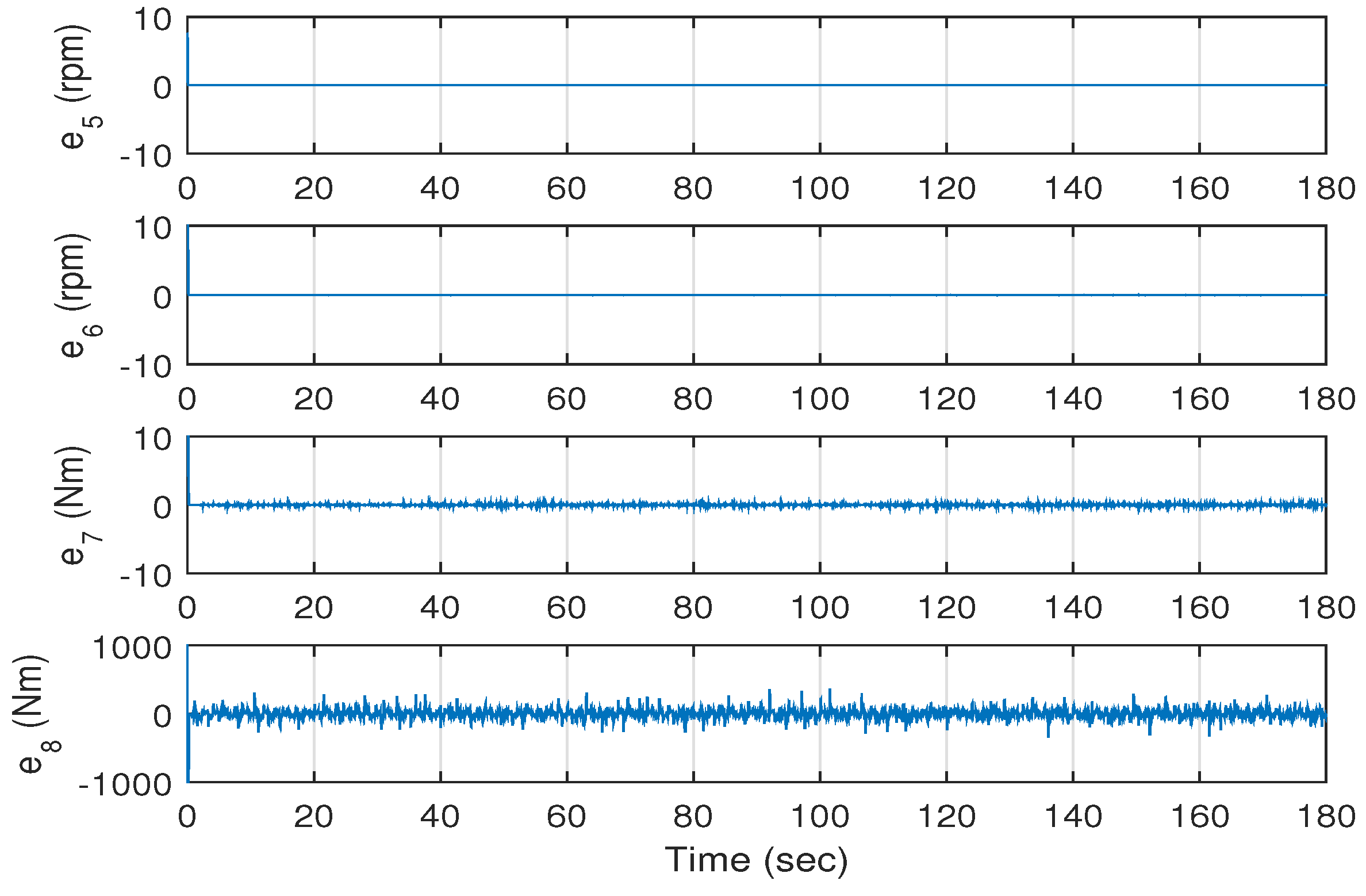
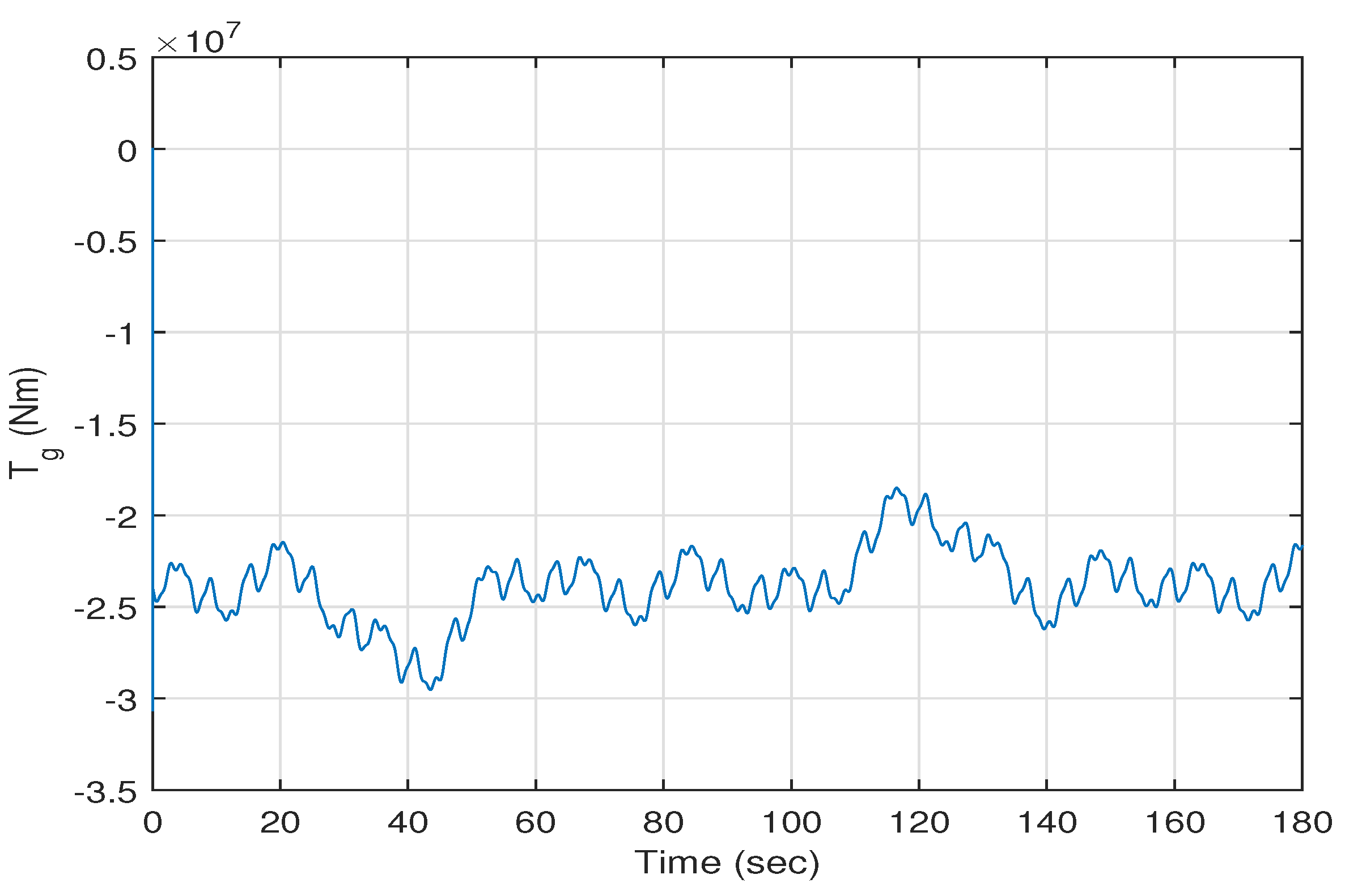
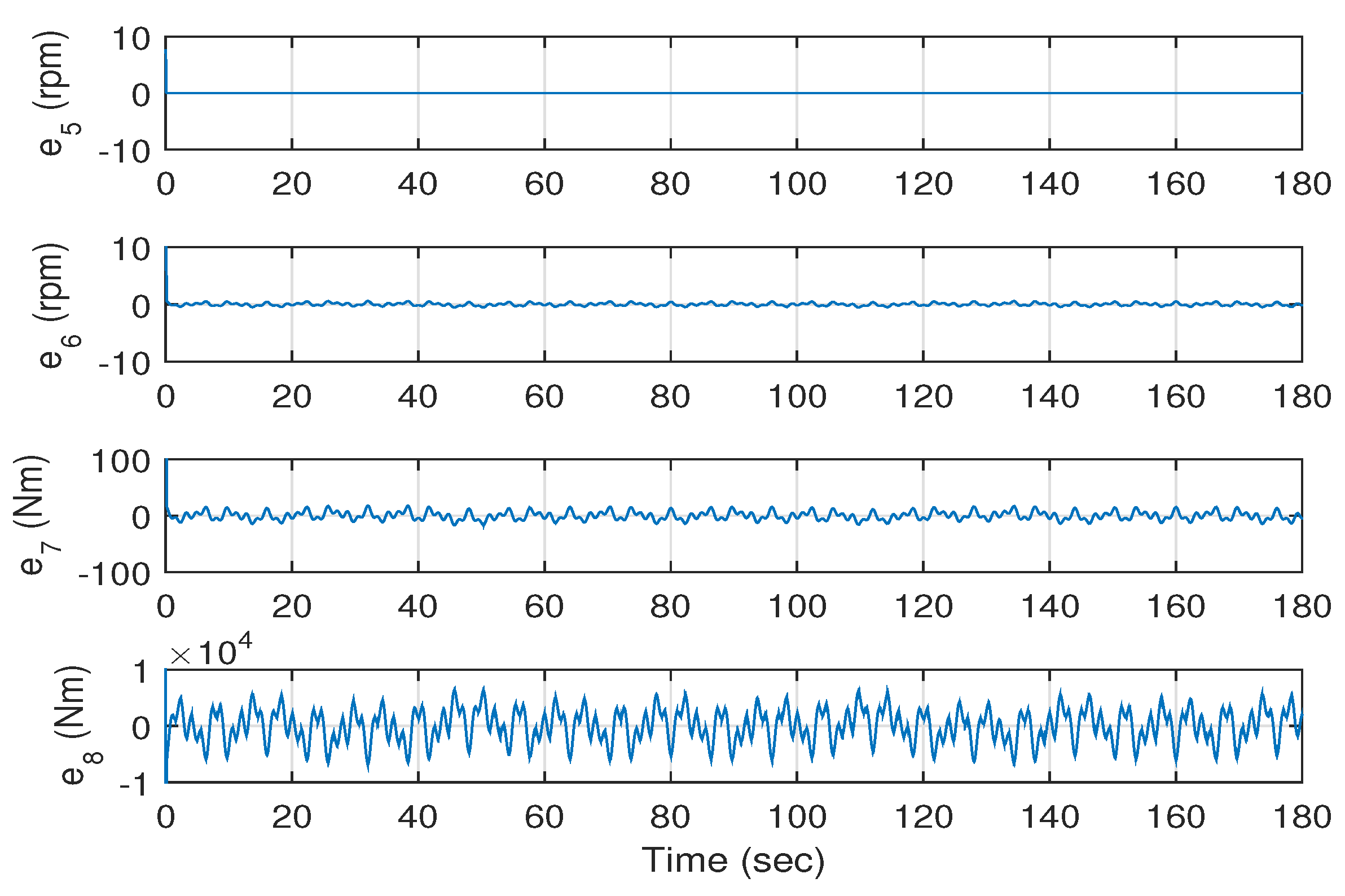
Figure 10 shows the errors of the mechanical states variables of the system. It is clear from this figure that the errors
and
converge to zero. However, the errors
and
show some fluctuations around zero; these fluctuations are due to the fact that their desired values are dependent on the wind speed. Note that the average value of the generated torque
is about
Nm. Therefore, it can be concluded that the states of the wind energy power system track the desired states.
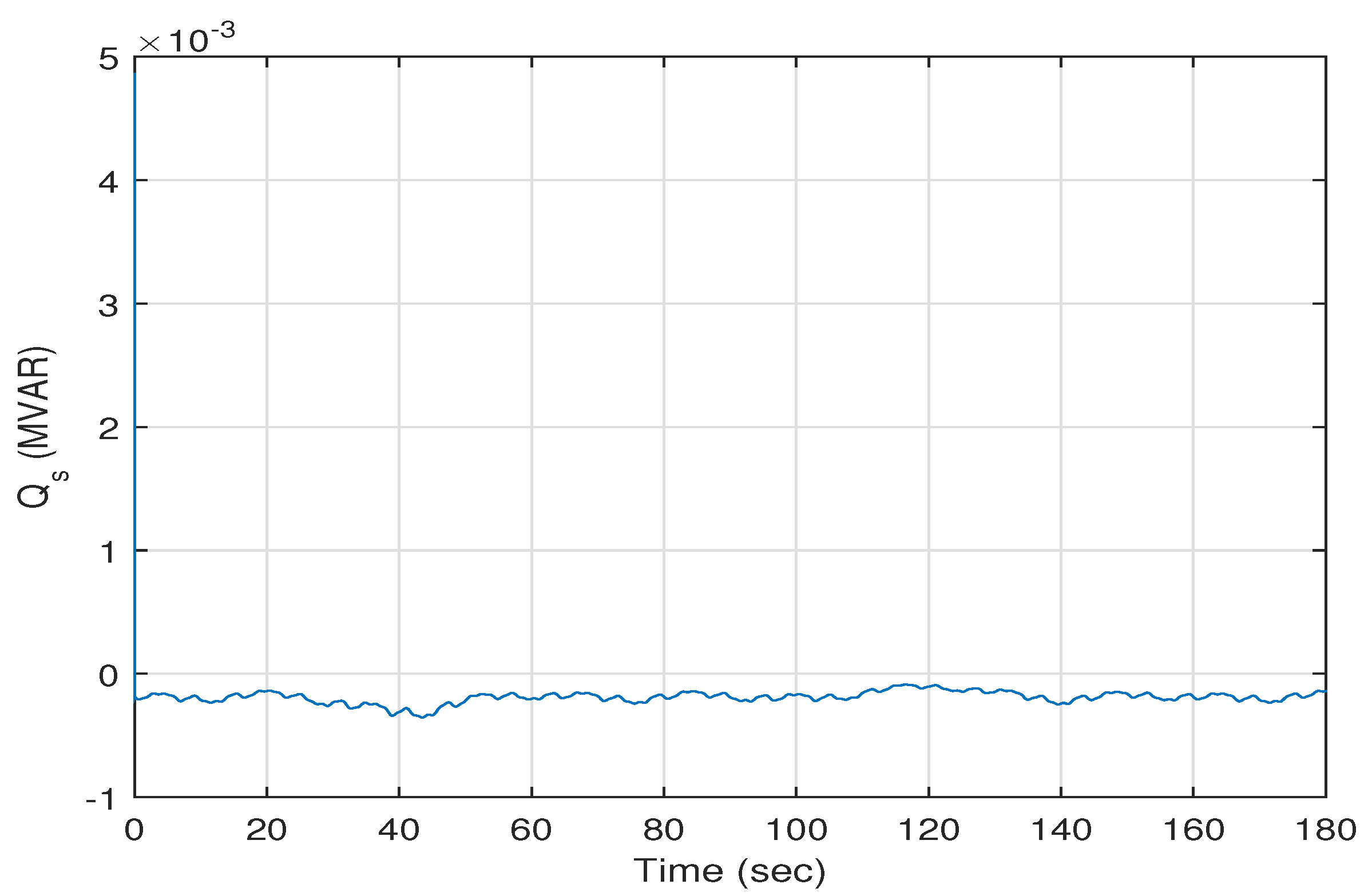
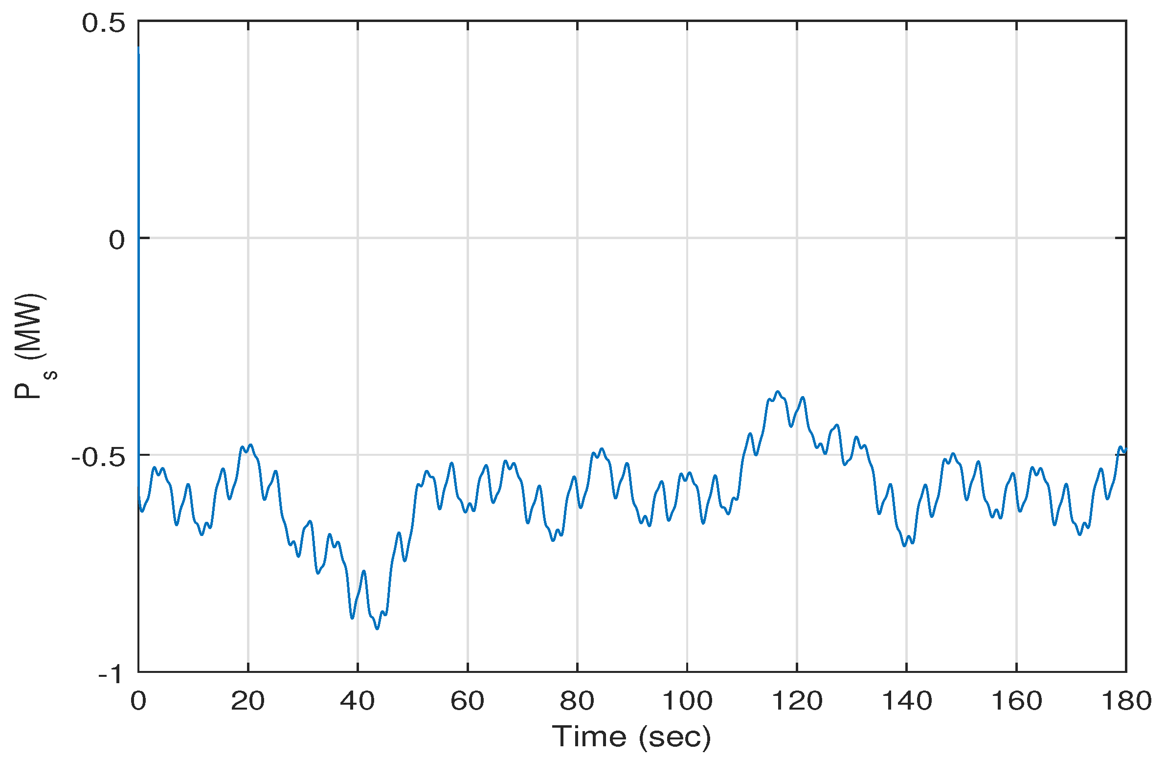
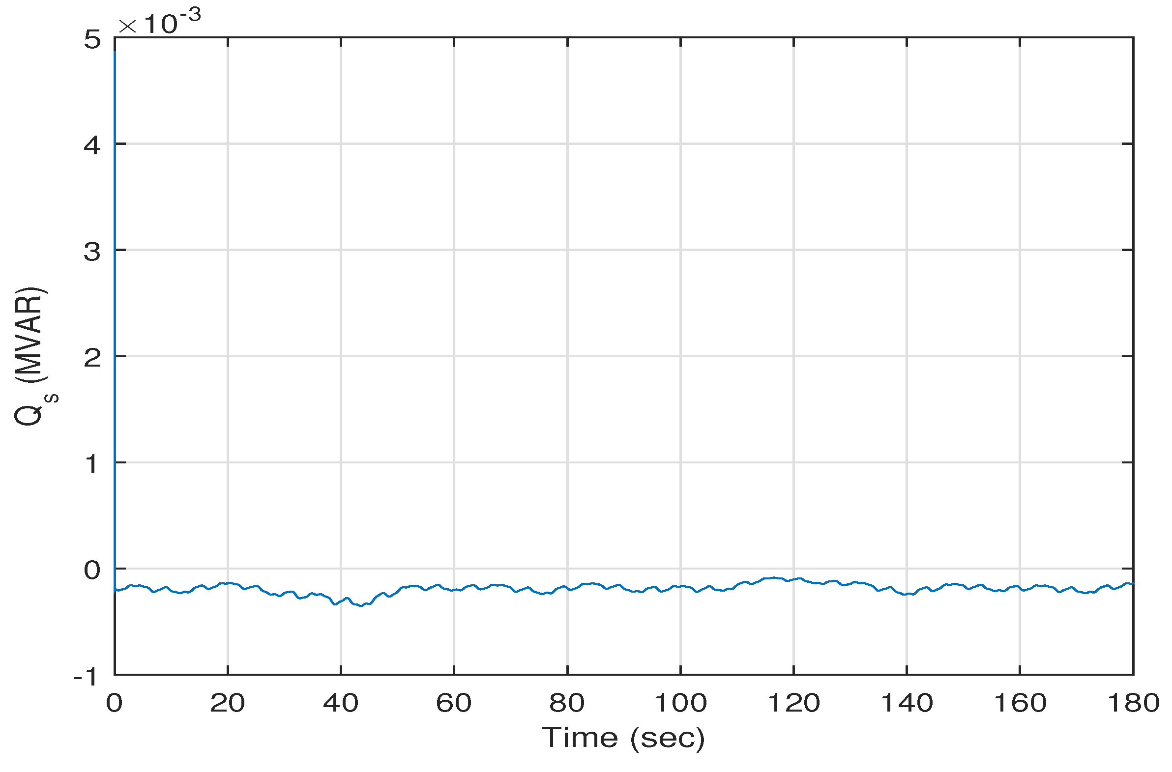
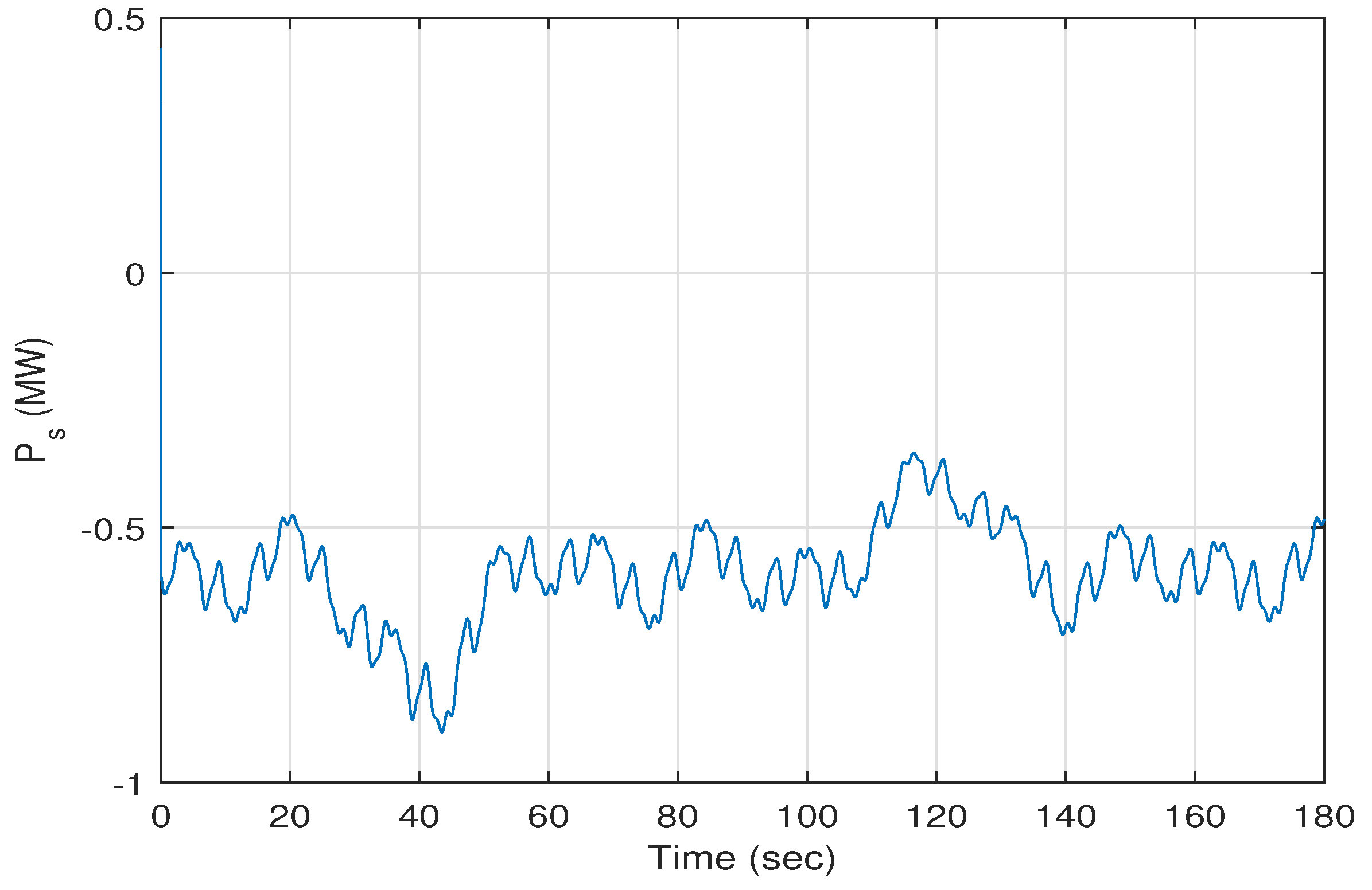
Figure 11 and
Figure 12 present the trajectories of the stator active and reactive powers
and
versus time. The average of the stator active power
is about −0.6 MW. The average of the stator reactive power
is about −0.002 MVAR.
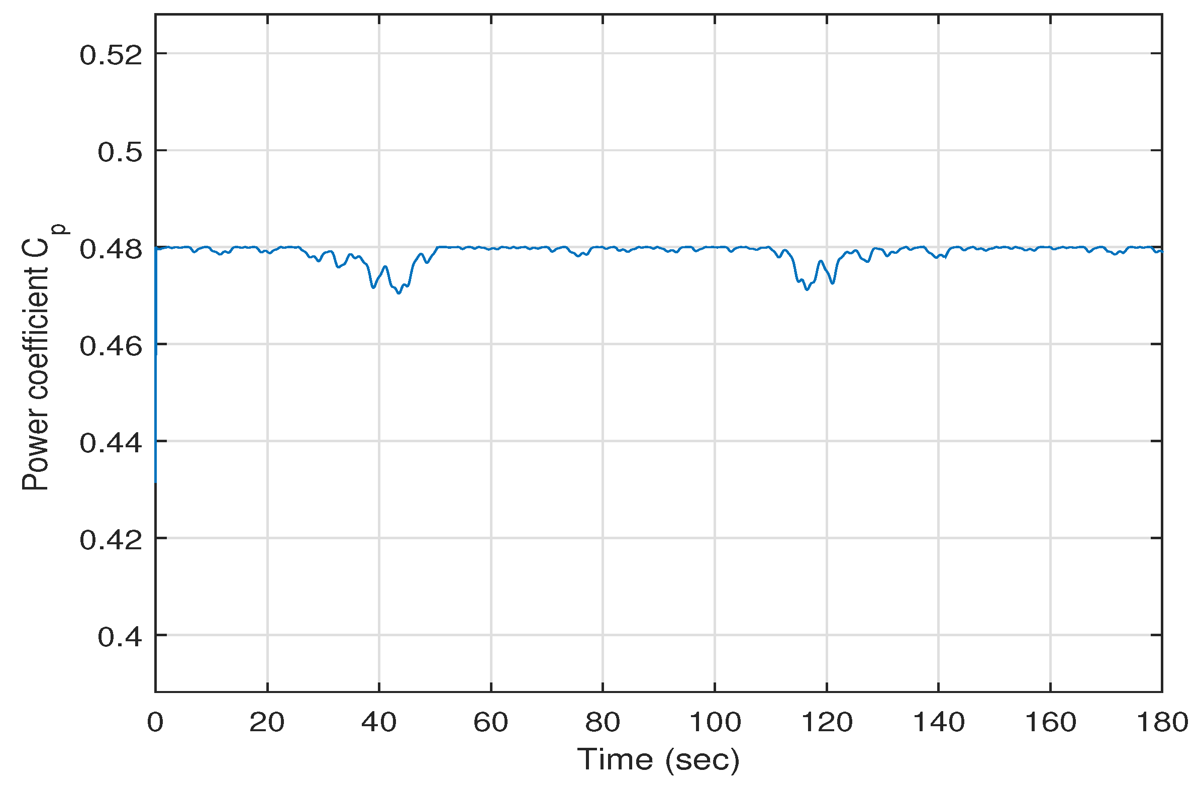
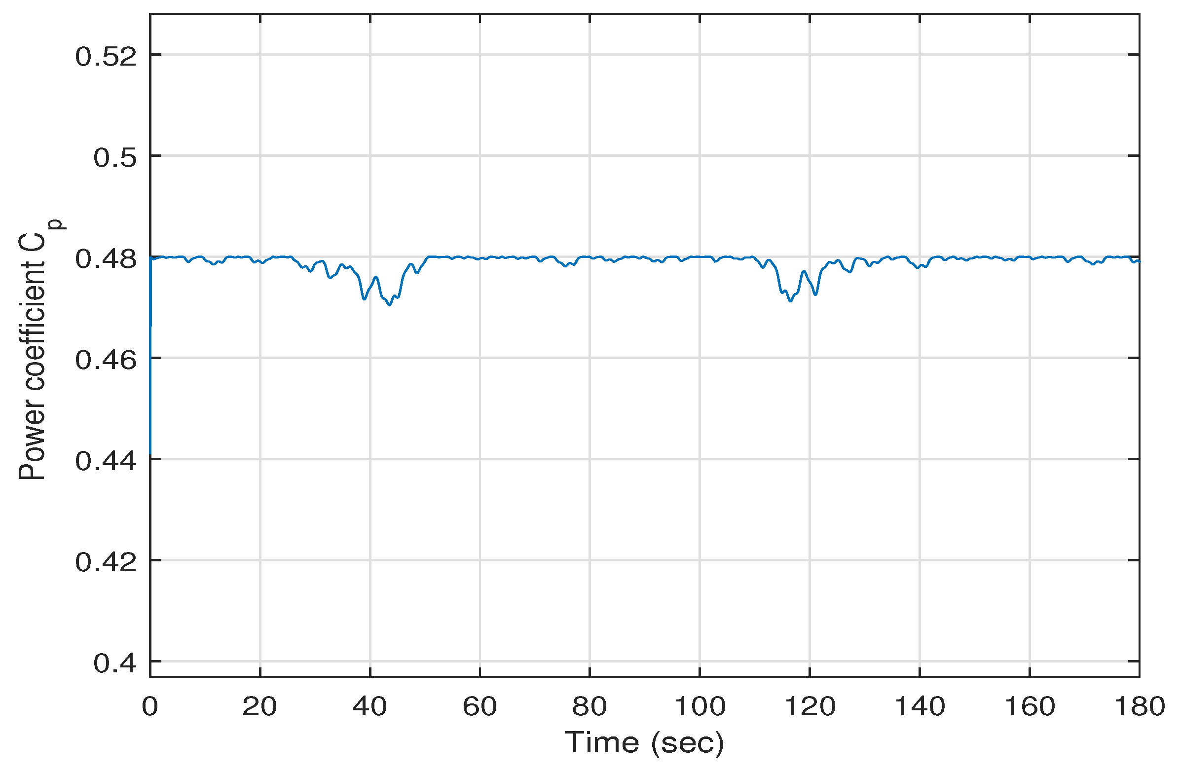
Figure 13 depicts the power coefficient
versus time; it is clear that the maximum value of the power coefficient is achieved when
. It is clear from these figures that all of the closed loop system signals are bounded and that all of the states of the power system converge to their desired values.
Therefore, it can be concluded that the simulation results indicate that the wind energy conversion system controlled using the proposed feedback linearization controller shows good performance.
5.2. Robustness of the Proposed Control Scheme
Simulation studies were carried out to investigate the robustness of the proposed control scheme to changes in some of the parameters of the wind energy conversion system. At first, the effects of the changes in the stator resistance , the rotor resistance and the rotor inductance are investigated. We simulated the performance of the closed loop system when the stator resistance , the rotor resistance and the rotor inductance are increased by of their nominal values. The responses of the system are not shown because of space limitations. However, the steady state performance of the system with the changed parameters is very similar to the steady state performance of the system with the nominal parameters. Hence, the change in some of the electrical parameters of the system did not affect the steady state performance of the system.
In addition, simulation studies were carried out to investigate the robustness of the proposed control scheme to changes in some of the electrical and some of the mechanical parameters of the wind energy conversion system. The effects of the changes in the stator resistance
, the rotor resistance
, the rotor inductance
, the moment of inertia of the rotor
and the moment of inertia of the generator
are investigated.
Figure 14,
Figure 15,
Figure 16,
Figure 17,
Figure 18,
Figure 19,
Figure 20,
Figure 21 and
Figure 22 show the system responses when the stator resistance
, the rotor resistance
and the rotor inductance
are increased by
; and when the moment of inertia of the rotor
and the moment of inertia of the generator
are increased by
of their nominal values.
Figure 14 and
Figure 15 show the rotor and the generator speed responses versus time. The high speed shaft torque and the generator torque versus time are shown in
Figure 16 and
Figure 17. The errors between the actual and the desired values of the eight states of the system are shown in in
Figure 18 and
Figure 19.
Figure 18 shows the errors of the electrical state variables of the system versus time. It is clear from this figure that the errors
,
and
converge to zero. However, the error
shows some fluctuations around zero.
Figure 19 shows the errors of the mechanical states variables of the system. It is clear from this figure that the error
converges to zero. However, the errors
,
and
show some fluctuations around zero. Note that in this case, the error
fluctuates between
and 10 Nm. The error
fluctuates between
and
Nm. The fluctuations in the error
seems to be high. However, it should be kept in mind that the average value of
is a bout
Nm. Even though the error is high in absolute value, it represents less than one percent of the value of
.
Figure 20 and
Figure 21 depict the stator active and reactive powers versus time.
Figure 22 depicts the power coefficient
. In this case, the reader can see the differences in the steady state performances of the system with the nominal parameters and the system with the changed parameters.
Hence, it can be concluded that the simulation results show that the proposed controller is robust to changes in some of the electrical parameters of the wind turbine conversion system. However, the simulation results indicate that the proposed controller is sensitive to changes in some parameters of the mechanical system.


