Hybridization of Chaotic Quantum Particle Swarm Optimization with SVR in Electric Demand Forecasting

Abstract

In existing forecasting research papers support vector regression with chaotic mapping function and evolutionary algorithms have shown their advantages in terms of forecasting accuracy improvement. However, for classical particle swarm optimization (PSO) algorithms, trapping in local optima results in an earlier standstill of the particles and lost activities, thus, its core drawback is that eventually it produces low forecasting accuracy. To continue exploring possible improvements of the PSO algorithm, such as expanding the search space, this paper applies quantum mechanics to empower each particle to possess quantum behavior, to enlarge its search space, then, to improve the forecasting accuracy. This investigation presents a support vector regression (SVR)-based load forecasting model which hybridizes the chaotic mapping function and quantum particle swarm optimization algorithm with a support vector regression model, namely the SVRCQPSO (support vector regression with chaotic quantum particle swarm optimization) model, to achieve more accurate forecasting performance. Experimental results indicate that the proposed SVRCQPSO model achieves more accurate forecasting results than other alternatives.

1. Introduction

Electric demand forecasting plays the critical role in the daily operational and economic management of power systems, such as energy transfer scheduling, transaction evaluation, unit commitment, fuel allocation, load dispatch, hydrothermal coordination, contingency planning load shedding, and so on [1]. Therefore, a given percentage of forecasting error implies great losses for the utility industries in the increasingly competitive market, as decision makers take advantage of accurate forecasts to make optimal action plans. As mentioned by Bunn and Farmer [2], a 1% increase in electric demand forecasting error represents a £10 million increase in operating costs. Thus, it is essential to improve the forecasting accuracy or to develop new approaches, particularly for those countries with limited energy [3].

In the past decades, many researchers have proposed lots of methodologies to improve electric demand forecasting accuracy, including traditional linear models, such as the ARIMA (auto-regressive integrated moving average) model [4], exponential smoothing models [5], Bayesian estimation model [6], state space and Kalman filtering technologies [7,8], regression models [9], and other time series technologies [10]. Due to the complexity of load forecasting, with these mentioned models it is difficult to illustrate well the nonlinear characteristics among historical data and exogenous factors, and they cannot always achieve satisfactory performance in terms of electric demand forecasting accuracy.

Since the 1980s, due to superior nonlinear mapping ability, the intelligent techniques like expert systems, fuzzy inference, and artificial neural networks (ANNs) [11] have become very successful applications in dealing with electric demand forecasting. In addition, these intelligent approaches can be hybridized to form new novel forecasting models, for example, the random fuzzy variables with ANNs [12], the hybrid Monte Carlo algorithm with the Bayesian neural network [13], adaptive network-based fuzzy inference system with RBF neural network [14], extreme learning machine with hybrid artificial bee colony algorithm [15], fuzzy neural network (WFNN) [16], knowledge-based feedback tuning fuzzy system with multi-layer perceptron artificial neural network (MLPANN) [17], and so on. Due to their multi-layer structure and corresponding outstanding ability to learn non-linear characteristics, ANN models have the ability to achieve more accurate performance of a continuous function described by Kromogol’s theorem. However, the main shortcoming of the ANN models are their structure parameter determination [18]. Complete discussions for the load forecasting modeling by ANNs are shown in references [19,20].

Support vector regression (SVR) [21], which has been widely applied in the electric demand forecasting field [11,22,23,24,25,26,27,28,29,30,31,32,33], hybridizes different evolutionary algorithms with various chaotic mapping functions (logistic function, cat mapping function) to simultaneously and carefully optimize the three parameter combination, to obtain better forecasting performance. As concluded in Hong’s series of studies, determination of these three parameters will critically influence the forecasting performance, i.e., low forecasting accuracy (premature convergence and trapped in local optimum) results from the theoretical limitations of the original evolutionary algorithms. Therefore, Hong and his successors have done a series of trials on hybridization of evolutionary algorithms with a SVR model. However, each algorithm has its embedded drawbacks, so to overcome these shortcomings, they continue applying chaotic mapping functions to enrich the searching ergodically over the whole space to do more compact searching in chaotic space, and also apply cloud theory to solve well the decreasing temperature problem during the annealing process to meet the requirement of continuous decrease in actual physical annealing processes, and then, improve the search quality of simulated annealing algorithms, eventually, improving the forecasting accuracy.

Inspired by Hong’s efforts mentioned above, the author considers the core drawback of the classical PSO algorithm, which results in an earlier standstill of the particles and loss of activities, eventually causing low forecasting accuracy, therefore, this paper continues to explore possible improvements of the PSO algorithm. As known in the classical PSO algorithm, the particle moving in the search space follows Newtonian dynamics [34], so the particle velocity is always limited, the search process is limited and it cannot cover the entire feasible area. Thus, the PSO algorithm is not guaranteed to converge to the global optimum and may even fail to find local optima. In 2004, Sun et al. [35] applied quantum mechanics to propose the quantum delta potential well PSO (QDPSO) algorithm by empowering the particles to have quantum behaviors. In a quantum system, any trajectory of any particles is non-determined, i.e., any particles can appear at any position in the feasible space if it has better fitness value, even far away from the current one. Therefore, this quantum behavior can efficiently enable each particle to expand the search space and to avoid being trapped in local minima. Many improved quantum-behaved swarm optimization methods have been proposed to achieve more satisfactory performance. Davoodi et al. [36] proposed an improved quantum-behaved PSO-simplex method (IQPSOS) to solve power system load flow problems; Kamberaj [37] also proposed a quantum-behaved PSO algorithm (q-GSQPO) to forecast the global minimum of potential energy functions; Li et al. [38] proposed a dynamic-context cooperative quantum-behaved PSO algorithm by incorporating the context vector with other particles while a cooperation operation is completed. In addition, Coelho [39] proposed an improved quantum-behaved PSO by hybridization with a chaotic mutation operator. However, like the PSO algorithm, the QPSO algorithm still easily suffers from shortcomings in iterative operations, such as premature convergence problems.

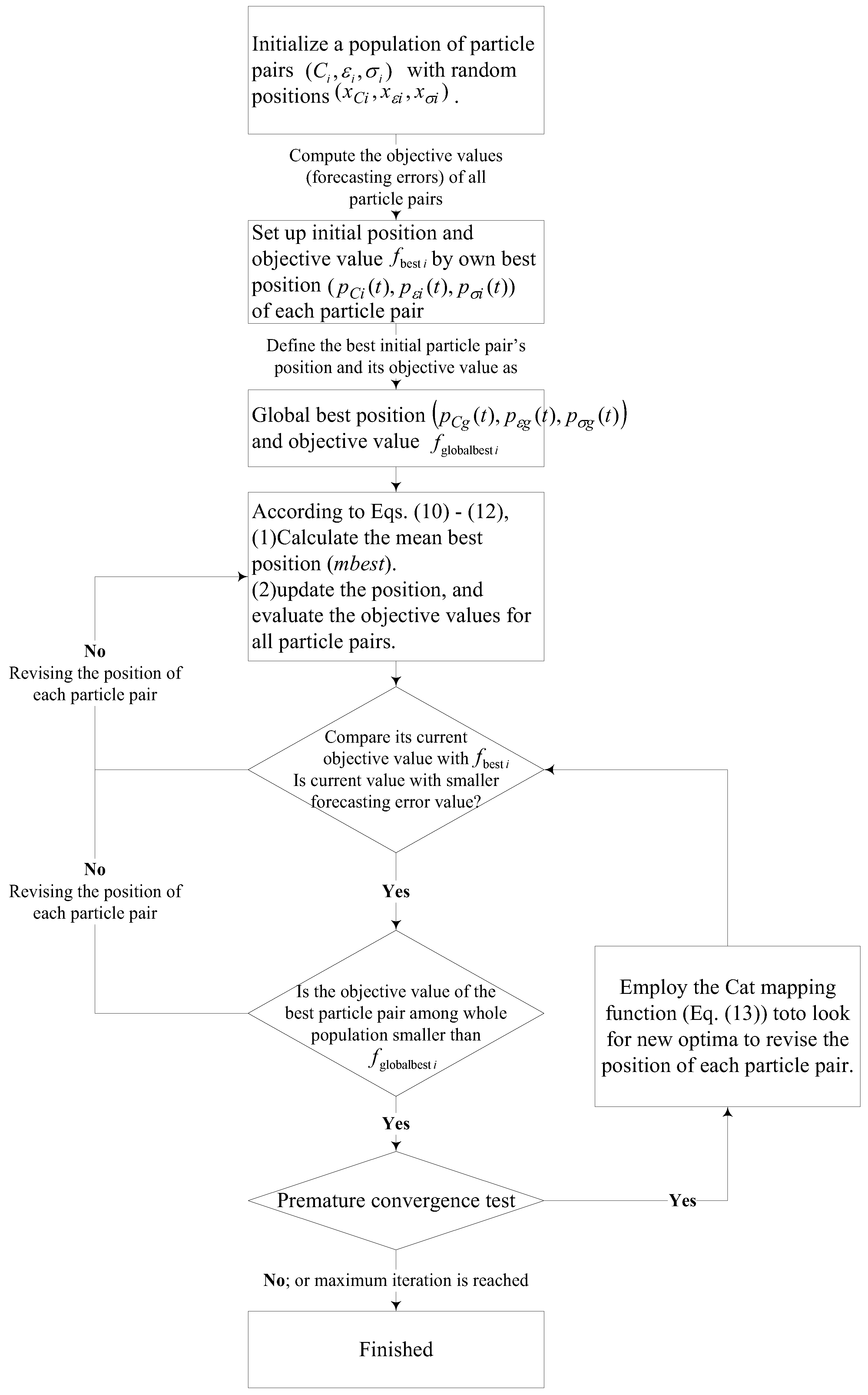
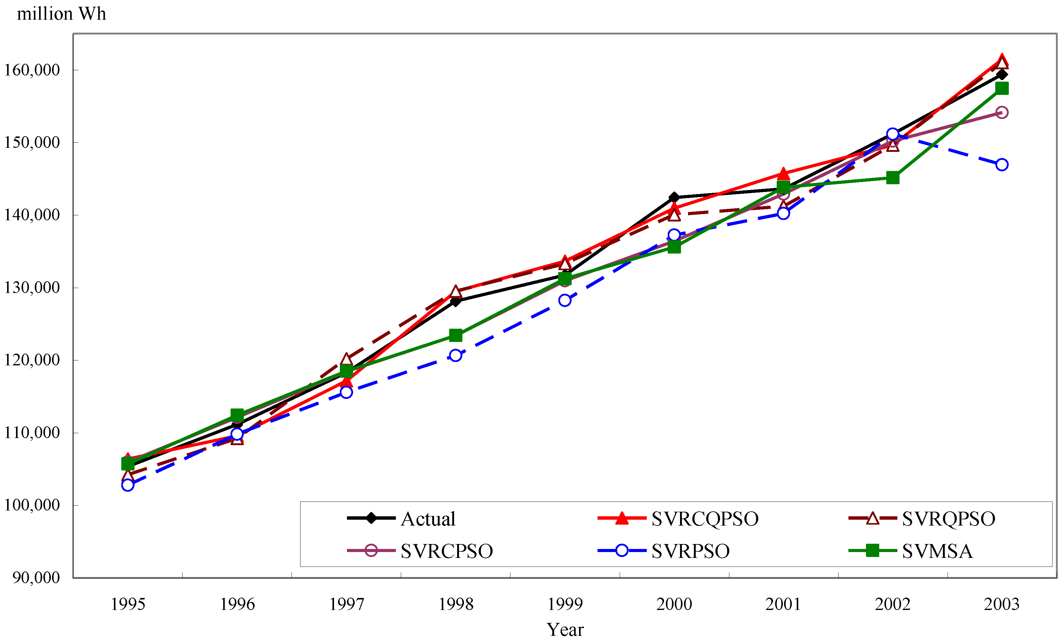
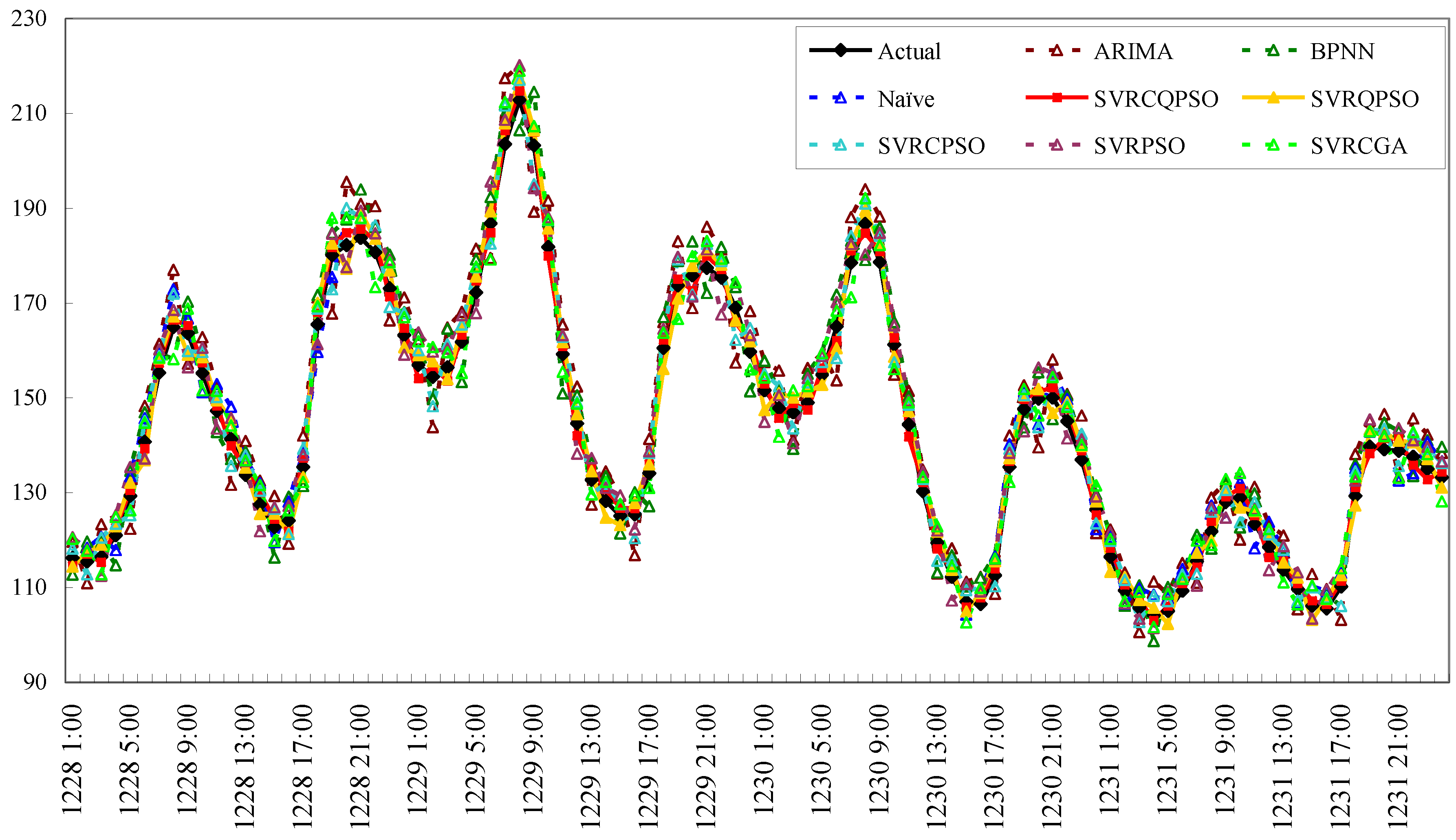
In this paper, the author applies quantum mechanics to empower each particle in the PSO algorithm to possess quantum behavior to enlarge the search space, then, a chaotic mapping function is employed to help the particles break away the local optima while the premature condition appears in each iterative searching process, eventually, improving the forecasting accuracy. Finally, the forecasting performance of the proposed hybrid chaotic quantum PSO algorithm with an SVR model, named SVRCQPSO model, is compared with four other existing forecasting approaches proposed in Hong [33] to illustrate its superiority in terms of forecasting accuracy.

This paper is organized as follows: Section 2 illustrates the detailed processes of the proposed SVRCQPSO model. The basic formulation of SVR, the QPSO algorithm, and the CQPSO algorithm will be further introduced. Section 3 employs two numerical examples and conducts the significant comparison among alternatives presented in an existing published paper in terms of forecasting accuracy. Finally, some meaningful conclusions are provided in Section 4.

2. Methodology of SVRCQPSO Model

2.1. Support Vector Regression (SVR) Model

The brief introduction of an SVR model is illustrated as follows. A nonlinear mapping function, $\mathsf{\varphi }(\cdot )$, is used to map the training data set into a high dimensional feature space. In the feature space, an optimal linear function, f, is theoretically found to formulate the relationship between training fed-in data and fed-out data. This kind of optimal linear function is called SVR function and is shown as Equation (1):

$$f(x)=w^{\mathrm{T}}\mathsf{\varphi }(x)+b$$

(1)

where $f(x)$ denotes the forecasting values; the coefficients w and b are adjustable. SVR method aims at minimizing the training error, that is the so-called empirical risk, as shown in Equation (2):

$$\begin{array}{ccc}\hfill R_{emp}(f)& =& \frac{1}{N}{\displaystyle \sum _{i=1}^N{\Theta }_{\mathsf{\epsilon }}(y_i,w^T\mathsf{\varphi }(x_i)+b)}\hfill \\ \hfill {\Theta }_{\mathsf{\epsilon }}(y,f(x))& =& \{\begin{array}{cc}\left|f(x)-y\right|-\mathsf{\epsilon },& \text{if}\begin{array}{c}\end{array}\left|f(x)-y\right|\ge \mathsf{\epsilon }\\ 0,& \text{otherwise}\end{array}\hfill \end{array}$$

(2)

where ${\Theta }_{\mathsf{\epsilon }}(y,f(x))$ is the $\mathsf{\epsilon }$-insensitive loss function. The $\mathsf{\epsilon }$-insensitive loss function is used to find out an optimum hyper plane on the high dimensional feature space to maximize the distance separating the training data into two subsets. Thus, the SVR focuses on finding the optimum hyperplane and minimizing the training error between the training data and the $\mathsf{\epsilon }$-insensitive loss function. The SVR model then minimizes the overall errors as shown in Equation (3):

$$\begin{array}{c}\begin{array}{c}\underset{w,b,{\mathsf{\xi }}^{*},\mathsf{\xi }}{\text{Min}}{R}_{\mathsf{\epsilon }}(w,{\mathsf{\xi }}^{*},\mathsf{\xi })=\frac{1}{2}{w}^{\mathrm{T}}w+C{\displaystyle \sum _{i=1}^N({\mathsf{\xi }}_i^{*}+{\mathsf{\xi }}_i)}\\ \text{with the constraints}\end{array}\\ \begin{array}{cc}{y}_i-w^{\mathrm{T}}\mathsf{\varphi }(x_i)-b\le \mathsf{\epsilon }+{\mathsf{\xi }}_i^{*},\hfill & i=1,2,\dots ,N\hfill \\ -y_i+w^{\mathrm{T}}\mathsf{\varphi }(x_i)+b\le \mathsf{\epsilon }+{\mathsf{\xi }}_i,\hfill & i=1,2,\dots ,N\hfill \\ {\mathsf{\xi }}_i^{*}\ge 0,\hfill & i=1,2,\dots ,N\hfill \\ {\mathsf{\xi }}_i\ge 0,\hfill & i=1,2,\dots ,N\hfill \end{array}\end{array}$$

(3)

The first term of Equation (3), by employed the concept of maximizing the distance of two separated training data, is used to regularize weight sizes, to penalize large weights, and to maintain regression function flatness. The second term, to penalize the training errors of f(x) and y, decides the balance between confidence risk and experience risk by using the $\mathsf{\epsilon }$-insensitive loss function. C is a parameter to trade off these two terms. Training errors above $\mathsf{\epsilon }$ are denoted as ${\mathsf{\xi }}_i^{*}$, whereas training errors below $-\mathsf{\epsilon }$ are denoted as ${\mathsf{\xi }}_i$.

After the quadratic optimization problem with inequality constraints is solved, the parameter vector w in Equation (1) is obtained with Equation (4):

$$w={\displaystyle \sum _{i=1}^N\left({\mathsf{\alpha }}_i^{*}-{\mathsf{\alpha }}_i\right)\mathsf{\varphi }(x_i)}$$

(4)

where ${\mathsf{\alpha }}_i^{*}$, ${\mathsf{\alpha }}_i$ are obtained by solving a quadratic program and are the Lagrangian multipliers. Finally, the SVR regression function is obtained as Equation (5) in the dual space:

$$f(x)={\displaystyle \sum _{i=1}^N\left({\mathsf{\alpha }}_i^{*}-{\mathsf{\alpha }}_i\right)K(x_i,x_j)}+b$$

(5)

where $K(x_i,x_j)$ is so-called the kernel function, and the value of the kernel equals the inner product of two vectors, $x_i$ and $x_j$, in the feature space $\mathsf{\varphi }(x_i)$ and $\mathsf{\varphi }(x_j)$, respectively; that is, $K(x_i,x_j)=\mathsf{\varphi }(x_i)\circ \mathsf{\varphi }(x_j)$. There are several types of kernel function, and it is hard to determine the best type of kernel functions for specific data patterns [40]. However, in practice, the Gaussian radial basis functions (RBF) with a width of $\mathsf{\sigma }$: $K(x_i,x_j)=\text{exp}\left(-0.5{\Vert x_i-x_j\Vert }^2/{\mathsf{\sigma }}^2\right)$ is not only easier to implement, but also capable of nonlinearly mapping the training data into an infinite dimensional space. Therefore, the Gaussian RBF kernel function is employed in this study.

It is well known that good determination of the three parameters (including hyperparameters, C, ε, and the kernel parameter, σ) in an SVR model will seriously affect its forecasting accuracy. Thus, to look for an efficient approach to simultaneously determine well the parameter combination is becoming an important research issue. As mentioned above, inspired by Hong’s series of efforts in hybridizing chaotic sequences with optimization algorithms for parameter determination to overcome the most embedded drawback of evolutionary algorithms—the premature convergence problem—this paper will continue exploring any solutions (such as empowering each particle with quantum behaviors) to overcome the embedded drawbacks of PSO, namely the QPSO algorithm, and the superiority of hybrid chaotic mapping function with the QPSO algorithms. Thus, the chaotic QPSO (CQPSO) algorithm is hybridized with an SVR model, named the SVRCQPSO model, to optimize the parameter selection to achieve more satisfactory forecasting accuracy.

2.2. Chaotic Quantum Particle Swarm Optimization Algorithm

2.2.1. Quantum Particle Swarm Optimization Algorithm

In the classical PSO algorithm, a particle’s action can be addressed completely by its position and velocity which determine the trajectory of the particle, i.e., any particles move along a deterministic trajectory in the search space by following Newtonian mechanics [34]. In the meanwhile, this situation also limits the possibility that the PSO algorithm could look for global optima and leads it to be trapped into local optima, i.e., premature convergence. To overcome this embedded drawback of the PSO algorithm, to solve the limitation of the deterministic particle trajectory, lots of efforts in the physics literature are focused on empowering each particle trajectory with stochasticity, i.e., empowering each particle’s movement with quantum mechanics.

Based on Heisenberg’s uncertainty principle [41], under quantum conditions, the position (x) and velocity (v) of a particle cannot be determined simultaneously, therefore, in the quantum search space, the probability of finding a particle at a particular position should be, via a “collapsing” process, mapped into its certain position in the solution space. Eventually, by employing the Monte Carlo method, the position of a particle can be updated using Equation (6):

$$x(t+1)=p(t)\pm \frac{1}{2}L(t)\text{ln}\left(\frac{1}{u(t)}\right)$$

(6)

where u(t) is a uniform random number distributed in [0, 1]; p(t) is the particle’s local attractor, and it is defined as Equation (7):

$$p(t)=\mathsf{\beta }{p}_{id}(t)+(1-\mathsf{\beta })p_{gd}(t)$$

(7)

where β is also a random number uniformly distributed in [0, 1]; p_id(t) and p_gd(t) are the ith pbest particle and the gbest particle in the dth dimension, respectively. L(t) is the length of the potential field [35], and is given by Equation (8):

$$L(t)=2\mathsf{\gamma }\left|p(t)-x(t)\right|$$

(8)

where parameter γ is the so-called the creativity coefficient or contraction expansion coefficient, and is used to control the convergence speed of the particle. QPSO algorithm can obtain good results by linear decreasing value of γ from 1.0 to 0.5, as shown in Equation (9) [42]:

$$\mathsf{\gamma }=(1-0.5)\times (Ite{r}_{\text{max}}-t)/Ite{r}_{\text{max}}+0.5$$

(9)

where Iter_max is the maximum of iteration numbers, in this paper, it is set as 10,000.

Considering that the critical position of L(t) will seriously influence the convergence rate and the performance of the QPSO algorithm, thus, we define the mean best position (mbest) as the center of pbest position of the swarm, shown in Equation (10):

$$\begin{array}{ll}m\text{best}(t)& =(m{\text{best}}_1(t), m{\text{best}}_2(t), \dots , m{\text{best}}_D(t)\\ & =\left(\frac{1}{S}{\displaystyle \sum _{i=1}^S{p}_{i1}(t)}, \frac{1}{S}{\displaystyle \sum _{i=1}^S{p}_{i2}(t)}, \dots , \frac{1}{S}{\displaystyle \sum _{i=1}^S{p}_{iD}(t)}\right)\end{array}$$

(10)

where S is the size of population, D is the number of dimensions, p_ij(t) is the pbest position of each particle in the jth dimension.

Then, we use Equation (10) to replace the p(t) in Equation (8), thus, the new evaluation equation of L(t) is Equation (11):

$$L(t)=2\mathsf{\gamma }\left|m\text{best}(t)-x(t)\right|$$

(11)

Finally, by substituting Equations (7) and (11) into Equation (6), the particle’s position is updated by Equation (12):

$$x(t+1)=\mathsf{\beta }{p}_{id}(t)+(1-\mathsf{\beta })p_{gd}(t)\pm \mathsf{\gamma }\left|m\text{best}(t)-x(t)\right|\text{ln}\left(\frac{1}{u(t)}\right)$$

(12)

2.2.2. Chaotic Mapping Function for QPSO Algorithm

As mentioned that chaotic variable can be adopted by applying chaotic phenomenon in keeping the diversities among particles to prevent the PSO algorithm from being trapped into a local optima, i.e., premature convergence. Therefore, the CQPSO algorithm is based on the QPSO algorithm by employing chaotic strategy while premature convergence appears during the iterative searching processes, else, the QPSO algorithm is still implemented as illustrated in Section 2.2.1.

On the other hand, for strengthening the effect of chaotic characteristics, lots of studies mostly apply the logistic mapping function as chaotic sequence generator. The biggest disadvantage of the logistic mapping function is that it distributes at both ends and less in the middle. On the contrary, the Cat mapping function has better chaotic distribution characteristic, thus, its application in chaos disturbance of the PSO algorithm can better strengthen the swarm diversity [43]. Therefore, this paper will employ the Cat mapping function as chaotic sequence generator.

The classical Cat mapping function is the two-dimensional Cat mapping function [44], shown as Equation (13):

$$\{\begin{array}{l}{x}_{n+1}=(x_n+y_n)\text{mod }1\\ y_{n+1}=(x_n+2y_n)\text{mod }1\end{array}$$

(13)

where x mod 1 = x − [x], mod, the so-called modulo operation, is used for the fractional parts of a real number x by subtracting an appropriate integer.

2.2.3. Implementation Steps of CQPSO Algorithm

The procedure of hybrid CQPSO algorithm with an SVR model is illustrated as follows and the corresponding flowchart is shown as Figure 1.

• Step 1: Initialization.

Initialize a defined population of particle pairs $\left(C_i,{\mathsf{\epsilon }}_i,{\mathsf{\sigma }}_i\right)$ with random positions $\left(x_{Ci},x_{\mathsf{\epsilon }i},x_{\mathsf{\sigma }i}\right)$, where each particle contains n variables.

• Step 2: Objective Values.

Compute the objective values (forecasting errors) of all particle pairs. Let the particle’s own best position be $p_{id}\left(t\right)=\left(p_{Ci}(t),p_{\mathsf{\epsilon }i}(t),p_{\mathsf{\sigma }i}(t)\right)$ of each particle pair and its objective value $f_{\text{best} i}$ equal its initial position and objective value. Let the global best position be $p_{gd}(t)=\left(p_{Cg}(t),p_{\mathsf{\epsilon }g}(t),p_{\mathsf{\sigma }g}(t)\right)$ and its objective value $f_{\text{globalbest} i}$ equal to the best initial particle pair’s position and its objective value.

• Step 3: Calculate Objective Values.

Employ Equation (10) to calculate the mean best position (mbest), the center of pbest position of the three particle pairs, then, use Equations (11) and (12) to update the position for each particle pair, and calculate the objective values for all particle pairs.

• Step 4: Update.

For each particle pair, compare its current objective value with $f_{\text{best} i}$. If current value is better (with smaller forecasting accuracy index value), then, update $\left(p_{Ci}(t),p_{\mathsf{\epsilon }i}(t),p_{\mathsf{\sigma }i}(t)\right)$ and its objective value with the current position and objective value.

• Step 5: Determine the Best Position and Objective.

Determine the best particle pair of whole population based on the best objective value. If the objective value is smaller than $f_{\text{globalbest} i}$, then update $\left(p_{Cg}(t),p_{\mathsf{\epsilon }g}(t),p_{\mathsf{\sigma }g}(t)\right)$, and, use Equation (7) to update the particle pair’s local attractor. Finally, update its objective value with the current best particle pair’s position.

• Step 6: Premature Convergence Test.

Calculate the mean square error (MSE), shown as Equation (14), to evaluate the premature convergence status, set the expected criteria, δ:

$$\text{MSE}=\frac{1}{S}{{\displaystyle \sum _{i=1}^S\left(\frac{f_i-f_{avg}}{f}\right)}}^2$$

(14)

where f_i is the current objective value of the current particles; f_avg is average objective value of the current swarm; f can be obtained by Equation (15):

$$f=\text{max}\left\{1,\underset{\forall i\in S}{\text{max}}\left\{\left|f_i-f_{avg}\right|\right\}\right\}$$

(15)

If the value of MSE is less than δ, it can be seen that premature convergence appears. Thus, the Cat mapping function, Equation (13), is then employed to look for new optima, and set the new optimal value as the optimal solution of the current particles.

• Step 7: Stop Criteria.

If a stopping threshold (forecasting accuracy) is reached, then $\left(P_{Cg},P_{\mathsf{\epsilon }g},P_{\mathsf{\sigma }g}\right)$ and its $f_{\text{globalbest} i}$ would be determined; otherwise go back to Step 3.

In this paper, the mean absolute percentage error (MAPE) as the forecasting accuracy index, shown in Equation (16), is employed for calculating the objective value to determine suitable parameters in Steps 4 and 5 of QPSO algorithm:

$$\text{MAPE}=\frac{1}{N}{\displaystyle \sum _{i=1}^N\left|\frac{y_i-f_i}{y_i}\right|}\times 100\%$$

(16)

where N is the number of forecasting periods; $y_i$ is the actual value at period i; $f_i$ denotes is the forecasting value at period i.

3. Numerical Examples

3.1. Data Set of Numerical Examples

3.1.1. Regional Load Data

The first numerical example applies Taiwan regional electric demand data from an existing published paper [33] to construct the proposed SVRCQPSO model, and the forecasting accuracy of the proposed model and other alternatives is compared. Therefore, in this example, the total load values in four regions of Taiwan from 1981 to 2000 (20 years) serve as experimental data. To be based on the same comparison basis, these load data are divided into three subsets, the training data set (from 1981 to 1992, i.e., 12 load data), the validation data set (from 1993 to 1996, that is four load data), and the testing data set (from 1997 to 2000, i.e., four load data). The forecasting accuracy is measured by Equation (16).

During the training process, the rolling-based forecasting procedure proposed by Hong [33] is employed, which divides training data into two subsets, namely fed-in (eight load data) and fed-out (four load data) respectively. The training error can be obtained in each iteration. While training error is decreasing, the three parameters determined by QPSO algorithm are employed to calculate the validation error. Then, those parameters with minimum validation error are selected as the most appropriate candidates. Notice that the testing data set is never employed while modeling. Eventually, the desired four-years forecasting loads in each region are forecasted. Along with the smallest testing MAPE value, the proposed model is the most suitable model in this example.

3.1.2. Annual Load Data

The second numerical example also uses Taiwan annual electric demand data from an existing paper [33]. The total annual electric demand values from 1945 to 2003 (59 years) serve as the experimental data. To be based on the same comparison basis, these employed load data are also divided into three data sets, the training data set (from 1945 to 1984, i.e., 40 years), the validation data set (from 1985 to 1994, that is 10 years), and the testing data set (from 1995 to 2003, i.e., nine years). Similarly, the forecasting accuracy is also measured by MAPE. Meanwhile, the rolling-based forecasting procedure, the structural risk minimization principle to minimize the training error, the procedure to determine parameter combination, and so on, are also implemented the same as in the first numerical example.

3.1.3. Load Data in 2014 Global Energy Forecasting Competition (GEFCOM 2014)

The third numerical example is suggested to use the historical hourly load data issued in 2014 Global Energy Forecasting Competition [45]. The total hourly load values, from 00:00 1 December 2011 to 00:00 1 January 2012 (744 h), serve as experimental data. These load data are divided into three data sets, the training data set (from 01:00 1 December 2011 to 00:00 24 December 2011, i.e., 552 h load data), the validation data set (from 01:00 24 December 2011 to 00:00 18 December 2011, that is 96 h load data), and the testing data set (from 01:00 28 December 2011 to 00:00 1 January 2012, i.e., 96 h load data). Similarly, the forecasting accuracy is also measured by MAPE; the rolling-based forecasting procedure, the structural risk minimization principle to minimize the training error, and the procedure to determine parameter combination are also implemented as the same as in the previous two numerical examples.

3.2. The SVRCQPSO Load Forecasting Model

3.2.1. Parameter Setting in the CQPSO Algorithm

Proper tuning of control parameters for convergence of the classical PSO algorithm is not easy, on the contrary, there is only one parameter control in the CQPSO algorithm, i.e., the creativity coefficient or contraction expansion coefficient, γ, given by Equation (9). Other settings, such as the population sizes, are 20 in both examples; the total number of iterations (Iter_max) is both fixed as 10,000; $\mathsf{\sigma }\in \left[0,5\right]$, $\mathsf{\epsilon }\in \left[0,100\right]$ in both examples, $C\in \left[0,20000\right]$ in example one, $C\in \left[0,3\times {10}^{10}\right]$ in example two; δ is both set as 0.001.

3.2.2. Three Parameter Determination of SVRQPSO and SVRCQPSO Models in Regional Load Data

For the first numerical example, the potential models with well determined parameter values by QPSO algorithm and CQPSO algorithm which have the smallest testing MAPE value will be selected as the most suitable models. The determined parameters for four regions in Taiwan are illustrated in

Table 1. Parameters determination of SVRCQPSO and SVRQPSO models (example one).

Regions	SVRCQPSO Parameters			MAPE of Testing (%)
	σ	C	ε
Northern	10.0000	0.9000 × 1010	0.7200	1.1070
Central	10.0000	1.8000 × 1010	0.4800	1.2840
Southern	4.0000	0.8000 × 1010	0.2500	1.1840
Eastern	3.0000	1.2000 × 1010	0.3400	1.5940
Regions	SVRQPSO Parameters			MAPE of Testing (%)
	σ	C	ε
Northern	8.0000	1.4000 × 1010	0.6500	1.3370
Central	8.0000	0.8000 × 1010	0.4300	1.6890
Southern	4.0000	0.6000 × 1010	0.6500	1.3590
Eastern	12.0000	1.0000 × 1010	0.5600	1.9830

.

Meanwhile, based on the same forecasting duration in each region,

Table 2. Forecasting results of SVRCQPSO, SVRQPSO, and other models (example one) (unit: 10⁶ MWh).

Year	Northern Region
	Actual	SVRCQPSO	SVRQPSO	SVRCPSO	SVRPSO	SVMG	RSVMG
1997	11,222	11,339	11,046	11,232	11,245	11,213	11,252
1998	11,642	11,779	11,787	11,628	11,621	11,747	11,644
1999	11,981	11,832	12,144	12,016	12,023	12,173	12,219
2000	12,924	12,798	12,772	12,306	12,306	12,543	12,826
MAPE (%)	-	1.1070	1.3370	1.3187	1.3786	1.3891	0.7498
Year	Central Region
	Actual	SVRCQPSO	SVRQPSO	SVRCPSO	SVRPSO	SVMG	RSVMG
1997	5061	4987	5140	5066	5085	5060	5065
1998	5246	5317	5342	5168	5141	5203	5231
1999	5233	5172	5130	5232	5236	5230	5385
2000	5633	5569	5554	5313	5343	5297	5522
MAPE (%)	-	1.2840	1.6890	1.8100	1.9173	1.8146	1.3026
Year	Southern Region
	Actual	SVRCQPSO	SVRQPSO	SVRCPSO	SVRPSO	SVMG	RSVMG
1997	6336	6262	6265	6297	6272	6265	6200
1998	6318	6401	6418	6311	6314	6389	6156
1999	6259	6179	6178	6324	6327	6346	6261
2000	6804	6738	6901	6516	6519	6513	6661
MAPE (%)	-	1.1840	1.3590	1.4937	1.5899	2.0243	1.7530
Year	Eastern Region
	Actual	SVRCQPSO	SVRQPSO	SVRCPSO	SVRPSO	SVMG	RSVMG
1997	358	353	350	370	367	358	367
1998	397	404	390	376	374	373	381
1999	401	394	410	411	409	397	401
2000	420	414	413	418	415	408	416
MAPE (%)	-	1.5940	1.9830	2.1860	2.3094	2.6475	1.8955

shows the MAPE values and forecasting results of various forecasting models in each region, including SVRCQPSO (hybridizing chaotic function, quantum mechanics, and PSO with SVR), SVRQPSO (hybridizing quantum mechanics and PSO with SVR), SVMG (hybridizing genetic algorithm with SVM), and RSVMG (hybridizing recurrent mechanism and genetic algorithm with SVM) models. In Table 2, the SVRQPSO model has almost outperformed SVRPSO models that hybridize classical PSO algorithm with an SVR model. It also demonstrates that empowering the particles to have quantum behaviors, i.e., applying quantum mechanics in the PSO algorithm, is a feasible approach to improve the solution, to improve the forecasting accuracy while the PSO algorithm is hybridized with an SVR model. In addition, the SVRCQPSO model eventually achieves a smaller MAPE value than other alternative models, except the RSVMG model in the northern region. It also illustrates that the Cat mapping function has done a good job of looking for more satisfactory solutions while suffering from the premature convergence problem during the QPSO algorithm processing. Once again, it also obviously illustrates the performance of the chaotic mapping function in overcoming the premature convergence problem. For example, in the northern region, we had done our best by using the QPSO algorithm, we could only to look for the solution, (σ, C, ε) = (8.0000, 1.4000 × 10¹⁰, 0.6500), with forecasting error, 1.3370%, as mentioned above that it is superior to classical PSO algorithm. However, the solution still could be improved by the CQPSO algorithm to (σ, C, ε) = (10.0000, 0.9000 × 10¹⁰, 0.7200) with more accurate forecasting performance, 1.1070%. Similarly, for other regions, the solutions of the QPSO algorithm with forecasting errors, 1.6890% (the central region), 1.3590% (the southern region) and 1.9830% (the eastern region), all could be further searched for more accurate forecasting performance by applying the Cat mapping function, i.e., the CQPSO algorithm, to receive more satisfactory results, such as 1.2840% (the central region), 1.1840% (the southern region), and 1.5940% (the eastern region), respectively.

Furthermore, to ensure the significant improvement in forecasting accuracy for the proposed SVRQPSO and SVRCQPSO models, as Diebold and Mariano [46] recommend, a suitable statistical test, namely the Wilcoxon signed-rank test, is then implemented. The test can be implemented at two different significance levels, i.e., α = 0.025 and α = 0.05, by one-tail-tests. The test results are shown in

Table 3. Wilcoxon signed-rank test (example one).

Compared Models	Wilcoxon Signed-Rank Test
	α = 0.025; W = 0				α = 0.05; W = 0
	Northern Region	Central Region	Southern Region	Eastern Region	Northern Region	Central Region	Southern Region	Eastern Region
SVRCQPSO vs. SVMG	0 a	1	1	0 a	0 a	1	1	0 a
SVRCQPSO vs. RSVMG	1	1	0 a	0a	1	1	0 a	0 a
SVRCQPSO vs. SVRPSO	0 a	1	1	0 a	0 a	1	1	0 a
SVRCQPSO vs. SVRCPSO	0 a	1	1	0 a	0 a	1	1	0 a
SVRCQPSO vs. SVRQPSO	1	1	0 a	0 a	1	1	0 a	0 a

^a denotes that the SVRCQPSO model significantly outperforms other alternative models.

, which indicates that the SVRCQPSO model only achives significantly better performance than other alternatives in the northern and eastern regions in terms of MAPE. It also implies that in these two regions, the load tendency is approaching a mature status, i.e., in northern Taiwan, it is highly commercial and residential electricity usage type; in eastern Taiwan, the highly concentrated natural resources only reflects its low electricity usage type. In both regions, the electricity load tendency and trend no doubt could be easily captured by the proposed SVRCQPSO model, thus, the proposed SVRCQPSO model can significantly outperform other alternatives.

On the other hand, in the central and southern regions, the SVRCQPSO model almost could not achieve significant accuracy improvements compared to the other models. It also reflects the facts that these two regions in Taiwan are both high-density population centers, the electricity usage types would be very flexible almost along with population immigration or emigration, thus, although the proposed SVRCQPSO model captures the data tendencies this time, however, it could not guarantee it will also achieve highly accurate forecasting performance when new data is obtained. Therefore, this is also the next research topic.

3.2.3. Three Parameters Determination of SVRQPSO and SVRCQPSO Models in Annual Load Data

For the second numerical example, the processing steps are similar to the example one. The parameters in an SVR model will also be determined by the proposed QPSO algorithm and CQPSO algorithm. Then, the selected models would be with the smallest testing MAPE values. The determined parameters for annual loads in Taiwan (example two) are illustrated in

Table 4. Parameter determination of SVRCQPSO and SVRQPSO models (example two).

Optimization Algorithms	Parameters			MAPE of Testing (%)
	σ	C	ε
SA algorithm [46]	0.2707	2.8414 × 1011	39.127	1.7602
PSO algorithm [33]	0.2293	1.7557 × 1011	10.175	3.1429
CPSO algorithm [33]	0.2380	2.3365 × 1011	39.296	1.6134
QPSO algorithm	12.0000	0.8000 × 1011	0.380	1.3460
CQPSO algorithm	10.0000	1.5000 × 1011	0.560	1.1850

. For benchmarking comparison with other algorithms, Table 4 lists all results in relevant papers with SVR-based modeling, such as the Pai and Hong [47] proposed SVMSA model by employing SA algorithm and the Hong [33] proposed SVRCPSO and SVRPSO models by using the CPSO algorithm and PSO algorithm, respectively.

Figure 2 illustrates the real values and forecasting values of different models, including the hybridizing simulated annealing algorithm with SVM (SVMSA), SVRPSO, SVRCPSO, SVRQPSO, and SVRCQPSO models. In Table 4, similarly, the SVRQPSO model is superior to SVRPSO models that hybridize a classical PSO algorithm with an SVR model. Once again, it also demonstrates that applying quantum mechanics in the PSO algorithm is a feasible approach to improve the forecasting accuracy of any SVR-based forecasting model. In addition, the SVRCQPSO model eventually achieves the smallest MAPE value than other alternative models. Of course, the Cat mapping function provides its excellent improvement in overcoming the premature convergence problem. It can be clearly to see that based on the QPSO algorithm, we could only look for the solution, (σ, C, ε) = (12.0000, 0.8000 × 10¹¹, 0.380), with a 1.3460% forecasting error, although it is superior to the classical PSO algorithm. Then, the Cat mapping function is excellent to shift the solution of the QPSO algorithm to another better solution, (σ, C, ε) = (10.0000, 1.5000 × 10¹¹, 0.560) with a forecasting error of 1.1850%.

To verify the significance of the proposed SVRCQPSO model in this annual load forecasting example, similarly, the Wilcoxon signed-rank test is also taken into account. The test results are shown in

Table 5. Wilcoxon signed-rank test (example two).

Compared Models	Wilcoxon Signed-Rank Test
	α = 0.025; W = 5	α = 0.05; W = 8
SVRCQPSO vs. SVMSA	2 a	2 a
SVRCQPSO vs. SVRPSO	3 a	3 a
SVRCQPSO vs. SVRCPSO	2 a	2 a
SVRCQPSO vs. SVRQPSO	2 a	2 a

^a denotes that the SVRCQPSO model significantly outperforms other alternative models.

, which indicate that the SVRCQPSO model has completely achieved a more significant performance than other alternatives in terms of MAPE, i.e., the annual load tendency in Taiwan reflects an increasing trend due to the strong annual economic growth. The electricity load tendency and trend no doubt could be easily captured by the proposed SVRCQPSO model; therefore, the proposed SVRCQPSO model can significantly outperform other alternatives.

3.2.4. Three Parameter Determination of SVRQPSO and SVRCQPSO Models in GEFCOM 2014

For the third numerical example, the processing steps are to be conducted similarly. The determined parameters in an SVR model by the proposed QPSO algorithm and CQPSO algorithm will have the smallest MAPE values in the test data set. The determined parameters for GEFCOM 2014 (example three) are illustrated in

Table 6. Parameters determination of SVRCQPSO and SVRQPSO models (example three).

Optimization Algorithms	Parameters			MAPE of Testing (%)
	σ	C	ε
Naïve	23.000	43.000	0.6700	3.2200
CGA	19.000	28.000	0.2700	2.9100
PSO algorithm	7.000	34.000	0.9400	3.1500
CPSO algorithm	22.000	19.000	0.6900	2.8600
QPSO algorithm	9.000	42.000	0.1800	1.9600
CQPSO algorithm	19.000	35.000	0.8200	1.2900

. In addition, the parameters determined by other famous algorithms, such as GA, CGA, PSO, CPSO algorithms, are also listed in Table 6. Because GEFCOM 2014 load data is a completely new case for the author, to correctly assess the improvements of the proposed models, a naïve model is introduced, which is appropriately to be a random search of the hyper-parameters. Therefore, the randomly determined parameters are also illustrated in Table 6.

For the forecasting performance comparison, the author also considers two famous forecasting models, the ARIMA(0, 1, 1) model, and the back propagation neural networks (BPNN) model to conduct benchmark comparisons. Figure 3 illustrates the real values and forecasting results, including the ARIMA, BPNN, Naïve, SVRCGA, SVRPSO, SVRCPSO, SVRQPSO, and SVRCQPSO models. In Figure 3, it also indicates that the SVRQPSO model achives more accurate forecasting performance than the SVRPSO and SVRCPSO models that hybridize classical PSO algorithms or chaotic sequences with an SVR model. It also illustrates the application of quantum mechanics in the PSO algorithm is a potential approach to improve the performance issues of any SVR-based model. In addition, the SVRCQPSO model eventually achieves a smaller MAPE value than the SVRQPSO model.

Finally, the results of Wilcoxon signed-rank test are presented in

Table 7. Wilcoxon signed-rank test (example three).

Compared Models	Wilcoxon Signed-Rank Test
	α = 0.025; W = 2,328	α = 0.05; W = 2,328
SVRCQPSO vs. ARIMA	1612 a	1612 a
SVRCQPSO vs. BPNN	1715 a	1715 a
SVRCQPSO vs. Naïve	1650 a	1650 a
SVRCQPSO vs. SVRPSO	1713 a	1713 a
SVRCQPSO vs. SVRCPSO	1654.5 a	1654.5 a
SVRCQPSO vs. SVRQPSO	1700 a	1700 a
SVRCQPSO vs. SVRCGA	1767 a	1767 a

^a denotes that the SVRCQPSO model significantly outperforms other alternative models.

, which indicates that the proposed SVRCQPSO model achieves superior significance in terms of MAPE, i.e., the hourly electric load reflects a cyclic trend which is captured exactly by the proposed SVRCQPSO model; therefore, the proposed SVRCQPSO model can significantly outperform other alternatives.

4. Conclusions

This paper presents an SVR model hybridized with the chaotic Cat mapping function and quantum particle swarm optimization algorithm (CQPSO) for electric demand forecasting. The experimental results demonstrate that the proposed model obtains the best forecasting performance among other SVR-based forecasting models in the literature, even though overall the forecasting superiority does not meet the significance test. This paper applies quantum mechanics to empower particles to have quantum behaviors to improve the premature convergence of the PSO algorithm and then, improve the forecasting accuracy. Chaotic Cat mapping is also employed to help with unexpected trapping into local optima while the QPSO algorithm is working in its searching process. This paper also illustrates the good feasibility of hybridizing quantum mechanics to expand the search space which is usually limited by Newtonian dynamics. In future research, as mentioned in Section 3.2.2, how to enhance the power of the QPSO algorithm to capture the tendency changes of electricity load data along with population immigration or emigration to guarantee the SVRCQPSO model achieves highly accurate forecasting performance will be studied.

References

1. Xiao, L.; Wang, J.; Hou, R.; Wu, J. A combined model based on data pre-analysis and weight coefficients optimization for electrical load forecasting. Energy 2015, 82, 524–549. [Google Scholar] [CrossRef]
2. Bunn, D.W.; Farmer, E.D. Comparative models for electrical load forecasting. Int. J. Forecast. 1986, 2, 241–242. [Google Scholar]
3. Zhao, W.; Wang, J.; Lu, H. Combining forecasts of electricity consumption in China with time-varying weights updated by a high-order Markov chain model. Omega 2014, 45, 80–91. [Google Scholar] [CrossRef]
4. Lee, C.M.; Ko, C.N. Short-term load forecasting using lifting scheme and ARIMA models. Expert Syst. Appl. 2011, 38, 5902–5911. [Google Scholar] [CrossRef]
5. Taylor, J.W.; Snyder, R.D. Forecasting intraday time series with multiple seasonal cycles using parsimonious seasonal exponential smoothing. Omega 2012, 40, 748–757. [Google Scholar] [CrossRef]
6. Hippert, H.S.; Taylor, J.W. An evaluation of Bayesian techniques for controlling model complexity and selecting inputs in a neural network for short-term load forecasting. Neural Netw. 2010, 23, 386–395. [Google Scholar] [CrossRef] [PubMed]
7. Al-Hamadi, H.M.; Soliman, S.A. Short-term electric load forecasting based on Kalman filtering algorithm with moving window weather and load model. Electr. Power Syst. Res. 2004, 68, 47–59. [Google Scholar] [CrossRef]
8. Zheng, T.; Girgis, A.A.; Makram, E.B. A hybrid wavelet-Kalman filter method for load forecasting. Electr. Power Syst. Res. 2000, 54, 11–17. [Google Scholar] [CrossRef]
9. Dudek, G. Pattern-based local linear regression models for short-term load forecasting. Electr. Power Syst. Res. 2016, 130, 139–147. [Google Scholar] [CrossRef]
10. Li, H.Z.; Guo, S.; Li, C.J.; Sun, J.Q. A hybrid annual power load forecasting model based on generalized regression neural network with fruit fly optimization algorithm. Knowl. Based Syst. 2013, 37, 378–387. [Google Scholar] [CrossRef]
11. Hong, W.C. Electric load forecasting by seasonal recurrent SVR (support vector regression) with chaotic artificial bee colony algorithm. Energy 2011, 36, 5568–5578. [Google Scholar] [CrossRef]
12. Lou, C.W.; Dong, M.C. A novel random fuzzy neural networks for tackling uncertainties of electric load forecasting. Int. J. Electr. Power Energy Syst. 2015, 73, 34–44. [Google Scholar] [CrossRef]
13. Niu, D.X.; Shi, H.; Wu, D.D. Short-term load forecasting using bayesian neural networks learned by Hybrid Monte Carlo algorithm. Appl. Soft Comput. 2012, 12, 1822–1827. [Google Scholar] [CrossRef]
14. Hooshmand, R.A.; Amooshahi, H.; Parastegari, M. A hybrid intelligent algorithm based short-term load forecasting approach. Int. J. Electr. Power Energy Syst. 2013, 45, 313–324. [Google Scholar] [CrossRef]
15. Li, S.; Wang, P.; Goel, L. Short-term load forecasting by wavelet transform and evolutionary extreme learning machine. Electr. Power Syst. Res. 2015, 122, 96–103. [Google Scholar] [CrossRef]
16. Hanmandlu, M.; Chauhan, B.K. Load forecasting using hybrid models. IEEE Trans. Power Syst. 2011, 26, 20–29. [Google Scholar] [CrossRef]
17. Mahmoud, T.S.; Habibi, D.; Hassan, M.Y.; Bass, O. Modelling self-optimised short term load forecasting for medium voltage loads using tunning fuzzy systems and artificial neural networks. Energy Convers Manag. 2015, 106, 1396–1408. [Google Scholar] [CrossRef]
18. Suykens, J.A.K.; Vandewalle, J.; De Moor, B. Optimal control by least squares support vector machines. Neural Netw. 2001, 14, 23–35. [Google Scholar] [CrossRef]
19. Sankar, R.; Sapankevych, N.I. Time series prediction using support vector machines: A survey. IEEE Commun. Mag. 2009, 4, 24–38. [Google Scholar]
20. Hahn, H.; Meyer-Nieberg, S.; Pickl, S. Electric load forecasting methods: Tools for decision making. Eur. J. Oper. Res. 2009, 199, 902–907. [Google Scholar] [CrossRef]
21. Drucker, H.; Burges, C.C.J.; Kaufman, L.; Smola, A.; Vapnik, V. Support vector regression machines. Adv. Neural Inform. Process. Syst. 1997, 9, 155–161. [Google Scholar]
22. Chen, Y.H.; Hong, W.C.; Shen, W.; Huang, N.N. Electric load forecasting based on LSSVM with fuzzy time series and global harmony search algorithm. Energies 2016, 9, 70. [Google Scholar] [CrossRef]
23. Fan, G.; Peng, L.-L.; Hong, W.-C.; Sun, F. Electric load forecasting by the SVR model with differential empirical mode decomposition and auto regression. Neurocomputing 2016, 173, 958–970. [Google Scholar] [CrossRef]
24. Geng, J.; Huang, M.L.; Li, M.W.; Hong, W.C. Hybridization of seasonal chaotic cloud simulated annealing algorithm in a SVR-based load forecasting model. Neurocomputing 2015, 151, 1362–1373. [Google Scholar] [CrossRef]
25. Ju, F.Y.; Hong, W.C. Application of seasonal SVR with chaotic gravitational search algorithm in electricity forecasting. Appl. Math. Model. 2013, 37, 9643–9651. [Google Scholar] [CrossRef]
26. Fan, G.; Wang, H.; Qing, S.; Hong, W.C.; Li, H.J. Support vector regression model based on empirical mode decomposition and auto regression for electric load forecasting. Energies 2013, 6, 1887–1901. [Google Scholar] [CrossRef]
27. Hong, W.C.; Dong, Y.; Zhang, W.Y.; Chen, L.Y.; Panigrahi, B.K. Cyclic electric load forecasting by seasonal SVR with chaotic genetic algorithm. Int. J. Electr. Power Energy Syst. 2013, 44, 604–614. [Google Scholar] [CrossRef]
28. Zhang, W.Y.; Hong, W.C.; Dong, Y.; Tsai, G.; Sung, J.T.; Fan, G. Application of SVR with chaotic GASA algorithm in cyclic electric load forecasting. Energy 2012, 45, 850–858. [Google Scholar] [CrossRef]
29. Hong, W.C.; Dong, Y.; Lai, C.Y.; Chen, L.Y.; Wei, S.Y. SVR with hybrid chaotic immune algorithm for seasonal load demand forecasting. Energies 2011, 4, 960–977. [Google Scholar] [CrossRef]
30. Hong, W.C. Application of chaotic ant swarm optimization in electric load forecasting. Energy Policy 2010, 38, 5830–5839. [Google Scholar] [CrossRef]
31. Hong, W.C. Hybrid evolutionary algorithms in a SVR-based electric load forecasting model. Int. J. Electr. Power Energy Syst. 2009, 31, 409–417. [Google Scholar] [CrossRef]
32. Hong, W.C. Electric load forecasting by support vector model. Appl. Math. Model. 2009, 33, 2444–2454. [Google Scholar] [CrossRef]
33. Hong, W.C. Chaotic particle swarm optimization algorithm in a support vector regression electric load forecasting model. Energy Convers Manag. 2009, 50, 105–117. [Google Scholar] [CrossRef]
34. Kennedy, J.; Eberhart, R.C. Particle swarm optimization. In Proceedings of the IEEE International Conference on Neural Networks, Piscataway, NJ, USA, 27 November–1 December 1995; pp. 1942–1948.
35. Sun, J.; Feng, B.; Xu, W.B. Particle swarm optimization with particles having quantum behavior. In Proceedings of the IEEE Proceedings of Congress on Evolutionary Computation, Piscataway, NJ, USA, 19–23 June 2004; pp. 325–331.
36. Davoodi, E.; Haque, M.T.; Zadeh, S.G. A hybrid improved quantum-behaved particle swarm optimization—Simplex method (IQPSOS) to solve power system load flow problems. Appl. Soft Comput. 2014, 21, 171–179. [Google Scholar] [CrossRef]
37. Kamberaj, H. Q-Gaussian swarm quantum particle intelligence on predicting global minimum of potential energy function. Appl. Math. Comput. 2014, 229, 94–106. [Google Scholar] [CrossRef]
38. Li, Y.; Jiao, L.; Shang, R.; Stolkin, R. Dynamic-context cooperative quantum-behaved particle swarm optimization based on multilevel thresholding applied to medical image segmentation. Inform. Sci. 2015, 294, 408–422. [Google Scholar] [CrossRef]
39. Coelho, L.D.S. A quantum particle swarm optimizer with chaotic mutation operator. Chaos Solitons Fractals 2008, 37, 1409–1418. [Google Scholar] [CrossRef]
40. Amari, S.; Wu, S. Improving support vector machine classifiers by modifying kernel functions. Neural Netw. 1999, 12, 783–789. [Google Scholar] [CrossRef]
41. Heisenberg, W. Über den anschaulichen Inhalt der quantentheoretischen Kinematik und Mechanik. Z. Phys. 1927, 43, 172–198. (In German) [Google Scholar] [CrossRef]
42. Liu, F.; Zhou, Z. An improved QPSO algorithm and its application in the high-dimensional complex problems. Chemom. Intell. Lab. Syst. 2014, 132, 82–90. [Google Scholar] [CrossRef]
43. Li, M.; Hong, W.C.; Kang, H. Urban traffic flow forecasting using Gauss-SVR with cat mapping, cloud model and PSO hybrid algorithm. Neurocomputing 2013, 99, 230–240. [Google Scholar] [CrossRef]
44. Chen, G.; Mao, Y.; Chui, C.K. Asymmetric image encryption scheme based on 3D chaotic cat maps. Chaos Solitons Fractals 2004, 21, 749–761. [Google Scholar] [CrossRef]
45. 2014 Global Energy Forecasting Competition. Available online: http://www.drhongtao.com/gefcom/ (accessed on 28 May 2016).
46. Diebold, F.X.; Mariano, R.S. Comparing predictive accuracy. J. Bus. Econ. Stat. 1995, 13, 134–144. [Google Scholar]
47. Pai, P.F.; Hong, W.C. Support vector machines with simulated annealing algorithms in electricity load forecasting. Energy Convers Manag. 2005, 46, 2669–2688. [Google Scholar] [CrossRef]
Figure 1. Quantum particle swarm optimization flowchart.
Energies 09 00426 g001
Figure 2. Actual values and forecasting values of SVRCQPSO, SVRQPSO, and other models (example two).
Energies 09 00426 g002
Figure 3. Actual values and forecasting values of SVRCQPSO, SVRQPSO, and other models (example three).
Energies 09 00426 g003