A Complete and Simplified Datasheet-Based Model of PV Cells in Variable Environmental Conditions for Circuit Simulation

Abstract

The paper proposes two mathematical models of a photo-voltaic (PV) cell—the complete model and the simplified model—which can be used also for modeling a PV module or a PV string under any environmental condition. Both of them are based on the well-known five-parameters model, while the approach allows to write a new descriptive equation, whose terms are functions of the information always available in the modern datasheet of a PV module’s manufacturer. This implies that no pre-processing of the datasheet parameters is needed to use the proposed model, whichever the solar irradiance and the cell/module temperature are. Moreover, these models are interpreted from a circuital point of view, providing the electrical circuits constituted only by basic electrical components. Particularly, in order to take into account the variability of the environment parameters, several variable resistors and voltage-controlled sources are used. The proposed models are tested with the datasheet parameters of commercial PV modules.

1. Introduction

The energy performance of a photo-voltaic (PV) system depends on many environmental parameters, nevertheless two of them are mainly responsible: the solar irradiance and the cell temperature. The former strongly affects the short-circuit current, the latter the open-circuit voltage, and both of them affect the maximum power point (MPP). Therefore, any reliable model of a PV system must take into account these parameters for any type of investigation: monitoring of the performance [1], forecasting of the produced power [2], development and testing of maximum power point tracking algorithms [3], and so on. A reliable model is also needed to study defective PV cells [4]. In these cases the thermal issues are relevant to classify the size and the severity of the defects; the finite element approach to model some classes of defects in the PV cells can be found in [5,6,7].

There also exist several equivalent circuits based on a photocurrent source, one or more resistors, and one or more diodes. These topologies are characterized by several unknowns to be calculated, in fact the models are also classified with respect to the total number of unknowns. For example, the widely used “single-diode” model is also known as a “five-parameters” model, because it may be completely characterized by five parameters, as will be seen later. Similarly, the more detailed “double-diode” model is also known as a “seven-parameters” model, because just two other parameters have to be calculated in addition to those of the “five-parameters” model. Both of the previous models are based on the accuracy through three characteristic points of the current-voltage (I-V) curve (open-circuit condition, short-circuit condition, and MPP) [8]. Other models are based on five characteristic points; beside the previous three points, two other points are considered: midway between MPP and open-circuit condition, at one-half of the open circuit condition [9].

The drawback of the previous models is that the values of the components (resistors, diodes, etc.) are not reported in any manufacturers’ datasheet. Instead, the datasheets may contain electrical information and some temperature-dependent coefficients. Thus, almost always a pre-processing of the values reported in the datasheet is needed before using the five- or seven-parameters model. Several authors have investigated this issue and there already exist PV models based on manufacturer datasheet information [10,11,12,13]. Nevertheless, these models are mathematical-based and cannot be used directly in a circuit simulator, even if circuit simulation is nowadays very important for many applications, including the study of the PV systems [14]. For this aim, this paper proposes a scalable model of a PV cell, derived from the five-parameters model. After defining the mathematical model, the equations are interpreted from a circuit point of view, thus an electrical circuit is derived. Moreover, it can be implemented in a standard circuit simulator, because only basic analog components are used. The paper is organized as follows: Section 2 derives the complete model and the simplified model, Section 3 shows the lumped electrical circuits, Section 4 presents the simulation results, finally Section 5 draws the conclusions.

2. Proposed Scalable Model of a PV Cell

This section is constituted by two parts. The first one introduces the single diode model, the link to the main environment parameters (solar irradiance and temperature) and the formulas to scale the model. The second one derives the mathematical models of a PV cell, starting from the well-known five-parameters circuit model. The single terms of the descriptive equation are revised, taking into account the environmental conditions (ECs). Moreover, the approach is based only on the parameters usually available in a manufacturer’s PV module datasheet. In this way, the proposed models can be used without any preliminary processing of the information reported in the datasheet.

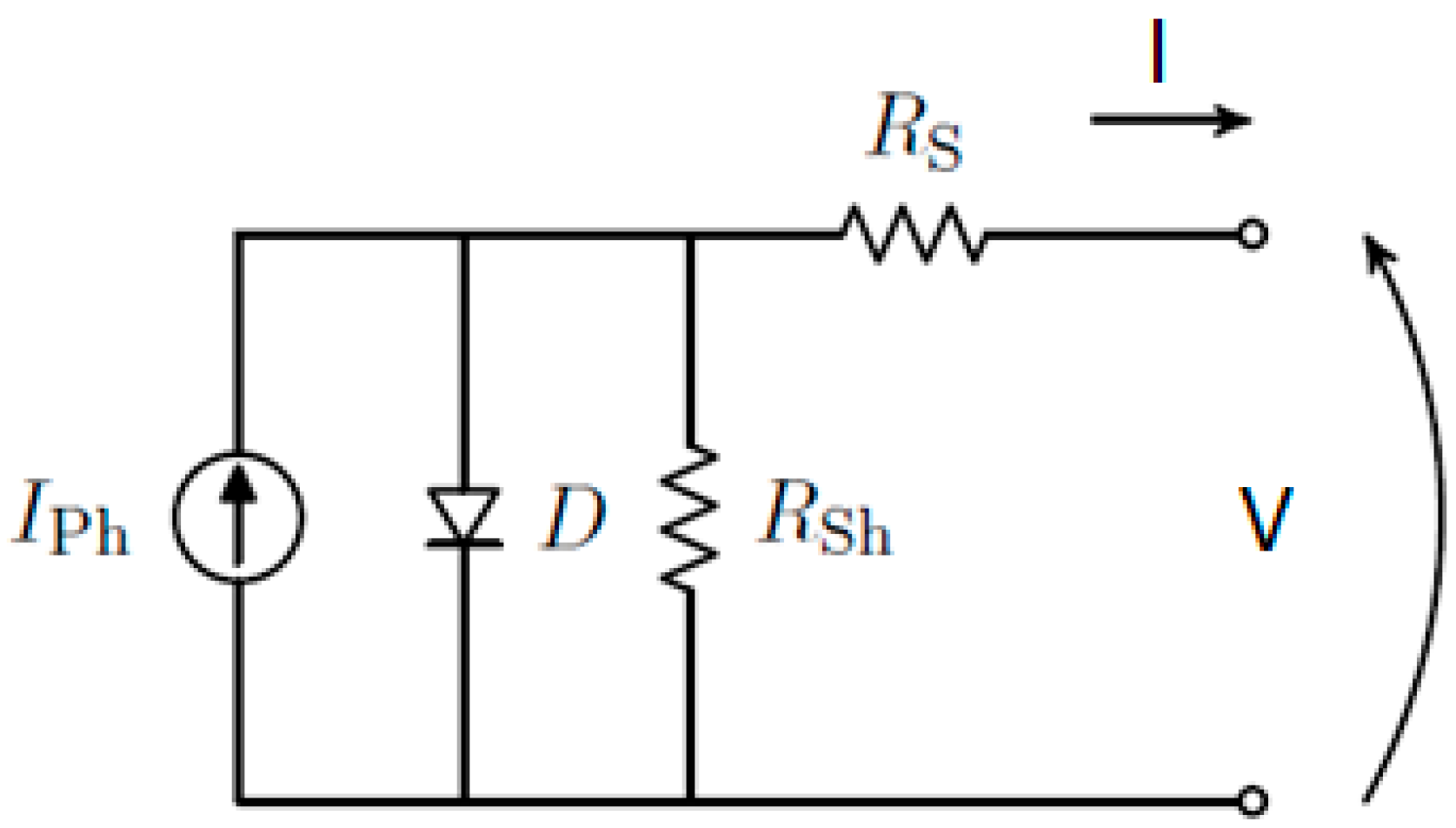
Figure 1 represents the well-known five-parameters model of a PV cell [8], whose descriptive equation is:

$$I=I_{Ph}-I_o\left(e^{-\frac{q\left(V+I·R_s \right)}{nk{T}_c}}-1\right)-\frac{V+I·R_s }{R_{sh}}$$

(1)

where I_Ph (A) is the light generated current (i.e., the short circuit current neglecting the parasitic resistances), I_o (A) is the dark saturation current due to recombination, q (C) is the electron charge, R_s (Ω) is a series resistance, n is the ideality factor, k (J/K) is the Boltzmann constant, T_c (K) is the cell temperature, and R_sh (Ω) is a shunt resistance. The five unknown parameters are R_s, R_sh, n, I_o, I_ph.

This model is valid for a fixed condition, but all the parameters are dependent on the ECs, primarily the solar radiance G and the air temperature T_a. Thus, Equation (1) can be used after determining the correct value of the parameters R_s, R_sh, n, I_o, I_ph under the actual ECs. Moreover, the values of these parameters are not available at all in the datasheets of the PV modules, where other specifications are usually shown and are related to the PV module and not to the PV cell vs. short-circuit current (I_sc), open-circuit voltage (V_oc), voltage and current in MPP (V_mpp and I_mpp), rated peak power (P_n), coefficients ${\mathsf{\alpha }}_{I_{sc}}$ (temperature coefficient for the short circuit current) and ${\mathsf{\alpha }}_{V_{oc}}$ (temperature coefficient for the open circuit voltage). All these parameters are defined in the standard test conditions (STCs), i.e., for solar radiation of 1000 W/m², air temperature T_a = 25 °C, air wind of 1 m/s and air mass AM = 1.5. Usually, also the nominal operating condition temperature (NOCT) is defined, but for 800 W/m² and cell temperature T_c of 20 °C. The NOCT is directly linked to T_a and T_c by the following expression:

$$T_c=T_a+\frac{G}{800}\times \left(\mathrm{NOCT}-20\right)$$

(2)

The datasheet contains also information about the number of series- and parallel-connected PV cells in the PV module, therefore it is easy to evaluate the characteristic currents and voltages of a PV cell using the corresponding values of the PV module:

$$V_{cell}=\frac{V_{module}}{N_s}$$

(3)

$$I_{cell}=\frac{I_{module}}{N_p}$$

(4)

being N_s the number of series-connected cells and N_p the number of parallel-connected groups of cells, respectively. Therefore, in the following we consider the voltage and the current of the PV cell satisfying Equations (3) and (4).

To summarize, the parameters of Figure 1 are not reported in the datasheet of the PV module and the parameters available are known only for a specific and fixed set of ECs. Therefore, the model in Figure 1 can be successfully used in a circuit simulator only after calculating the five parameters in the operating EC, thus a single simulation with variable EC cannot be run.

The aim of this paper is to propose an upgraded model of a PV cell, constituted by components depending on both the manufacturer datasheet and the operating ECs. In this way, it can be used in a circuit simulator for the analysis in variable Operating Conditions (OCs).

2.1. Mathematical Formulation of the Complete Model

The light generated current is directly proportional to the solar irradiance [15]:

$$I_{Ph}=G_{pu}·\left[I_{sc}^o+{\mathsf{\alpha }}_{I_{sc}}·\left(T_c-25\right)\right]$$

(5)

where G_pu = G/1000 is the relative solar irradiance referred to the STC value, $I_{sc}^o$ is the short circuit current and the superscript “o” stands for STC, ${\mathsf{\alpha }}_{I_{sc}}$ is the current-temperature coefficient at STC, ΔT = (T_c − 25) is the mismatch of the cell temperature with respect to the STC cell temperature.

The structure of Equation (5) is approximately valid also for the I_mpp:

$$I_{mpp}=G_{pu}·\left[I_{mpp}^o+{\mathsf{\alpha }}_{I_{sc}}·\left(T_c-25\right)\right]$$

(6)

The above equation states that the current in MPP depends on both the solar irradiance and the cell temperature.

Let us study the second term of Equation (1). The dark saturation current I_o depends on the cell temperature [16], whereas the series resistance R_s depends on the ECs [17]. Moreover, it has two characteristic values for V = 0 and V = V_oc, i.e., in short- and open-circuit condition. For these extreme values, it ranges from about zero to I_o, because the exponential term ranges from 1 to 0. This term can be represented as:

$$\mathsf{\beta }·e^{\mathsf{\gamma }·\left(V+{\mathsf{\alpha }}_{V_{oc}}·\Delta T-V_{oc}^o\right)}$$

(7)

where $V_{oc}^o$ is the open circuit voltage in STC, while β and γ are parameters to be calculated, as shown later, and ΔT = (T_c − 25), as already explained.

Equation (7) highlights that the open circuit voltage V_oc strongly depends on the cell temperature as [18]:

$$V_{oc}=V_{oc}^o-{\mathsf{\alpha }}_{V_{oc}}·\Delta T$$

(8)

Also for V_mpp the following mathematical relation is approximately valid:

$$V_{mpp}=V_{mpp}^o-{\mathsf{\alpha }}_{V_{oc}}·\Delta T$$

(9)

because the values of V_mpp and V_oc typically differ by less than 15%.

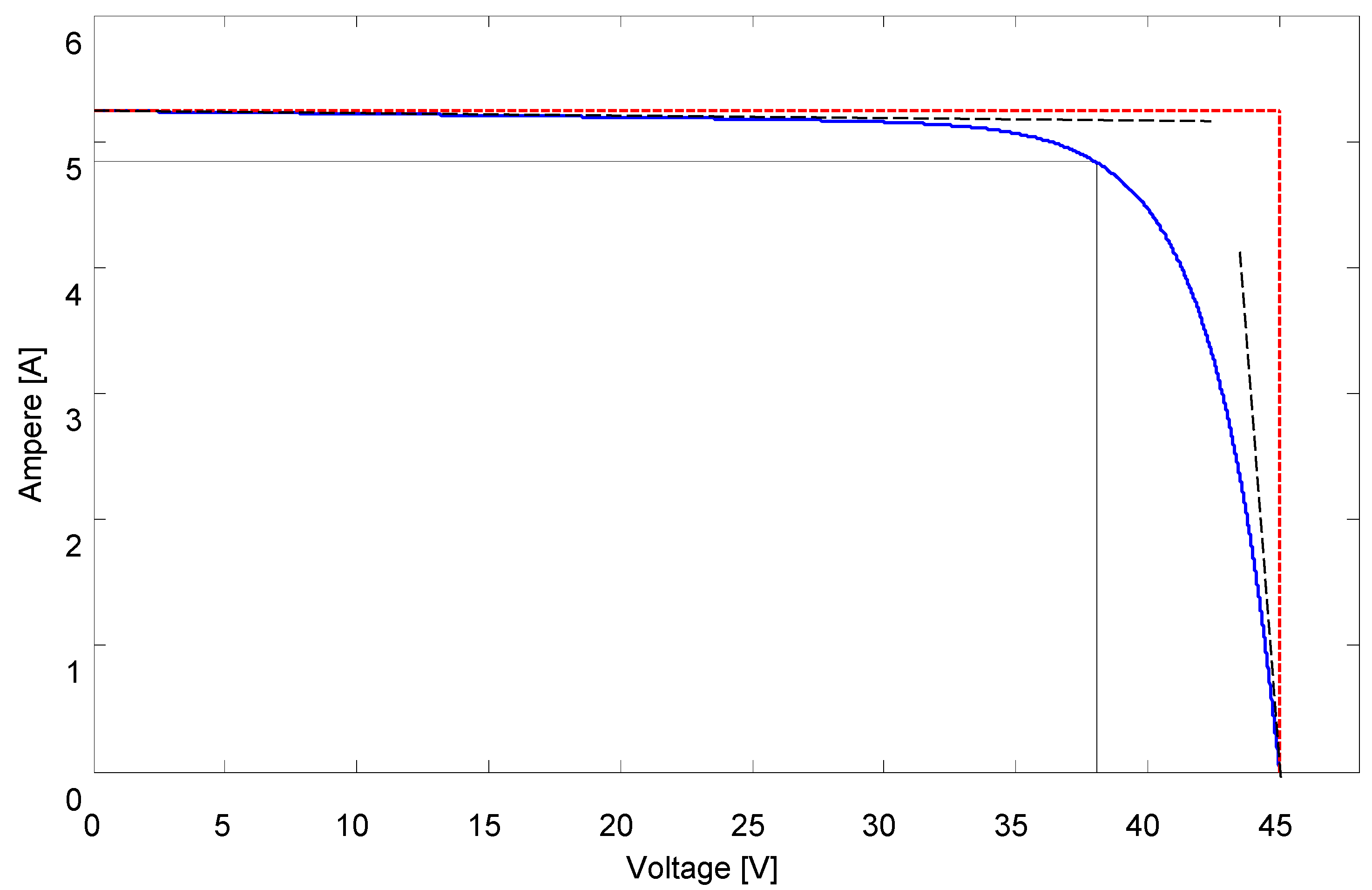
The last term of Equation (1) contains the dissipative resistors R_s and R_sh. These resistors do not represent components that actually exist in a PV cell, instead they model some dissipative phenomena of the PV cell/module (Table 2, page 91 of [17]). Figure 2 represents the typical I-V curve of a PV module (a set of PV cells connected in series and, sometimes, in parallel). The red lines are the asymptotes of the open- and short-circuit conditions, whereas the solid black lines define the MPP. From a graphical point of view, the resistance R_s is related the slope of the I-V curve in the open circuit condition (black dotted line), whereas R_sh is related to the slope in the short-circuit condition (black dotted line) [18].

For the sake of simplicity, the losses resistances was neglected in [19], thus assuming R_sh → ∞ and R_s = 0. Otherwise, this paper just studies the effects of the two resistances, upgrading the previous model introduced in [19]. For this aim, firstly the equations describing the values of the resistances are proposed and inserted into the general I-V equation, then the characteristic parameters are derived.

Since R_sh is related to the slope of the I-V curve in the short-circuit condition, it can be approximated (Figure 2) as:

$$R_{sh}=\frac{V_{mpp}^o-{\mathsf{\alpha }}_{V_{oc}}·\Delta T}{G_{pu}·\frac{\left(I_{sc}^o-I_{mpp}^o\right)}{2}}=\frac{V_{sh}}{I_{sh}}$$

(10)

Instead, R_s is related to the slope of the I–V curve in the open circuit condition, following (Figure 2):

$$R_s=\frac{\frac{\left(V_{oc}^o-V_{mpp}^o\right)}{4}}{G_{pu}·\left(I_{mpp}^o+{\mathsf{\alpha }}_{I_{sc}}·\Delta T\right)}=\frac{V_s}{I_s}$$

(11)

Finally, substituting Equations (5)–(7) into Equation (1) and taking into account Equations (10) and (11), Equation (12) that permits one to trace the I-V curve under arbitrary ECs follows. It can be seen that Equation (12) depends on the ECs, on the datasheet parameters, and on the β and γ parameters:

$$I·\left(1+\frac{R_s}{R_{sh}}\right)=G_{pu}·\left(I_{sc}^o+{\mathsf{\alpha }}_{I_{sc}}·\Delta T\right)-\mathsf{\beta }·e^{\mathsf{\gamma }·\left(V+{\mathsf{\alpha }}_{V_{oc}}·\Delta T-V_{oc}^o\right)}-\frac{V}{R_{sh}}$$

(12)

In order to evaluate β and γ, we impose some constraints to Equation (12), i.e., the values in the three most significant points:

$$\{\begin{array}{c}I =I_{sc} for V=0 \\ I=0 for V=V_{oc} \\ \frac{dP}{dV}=0 for V=V_{mpp} \end{array}$$

(13)

Solving Equation (13) gives:

$$I_{sc}=p·\left[G_{pu}·\left(I_{sc}^o+{\alpha }_{I_{sc}}·\Delta T\right)\right]$$

(14)

$$\mathsf{\beta }=G_{pu}·\left(I_{sc}^o+{\mathsf{\alpha }}_{I_{sc}}·\Delta T\right)-\frac{V_{oc}^o-{\mathsf{\alpha }}_{V_{oc}}·\Delta T}{R_{sh}}$$

(15)

$$\mathsf{\gamma }=\frac{1}{{\mathrm{V}}_{mpp}^{\mathrm{o}}-{\mathrm{V}}_{\mathrm{oc}}^{\mathrm{o}}}·log\frac{G_{pu}*\left(p{I}_{sc}^o-I_{mpp}^o\right)-\left(1-p\right)·{\alpha }_{I_{sc}}·\Delta T-\frac{p·\left(V_{mpp}^o-{\mathsf{\alpha }}_{V_{oc}}·\Delta T\right)}{R_{sh}}}{p·\left(G_{pu}·\left(I_{sc}^o+{\alpha }_{I_{sc}}·\Delta T\right)-\frac{V_{oc}^o-{\mathsf{\alpha }}_{V_{oc}}·\Delta T}{R_{sh}}\right)}$$

(16)

where $p=\frac{R_{sh}}{R_s+R_{sh}}=\frac{\left(V_{mpp}^o-{\mathsf{\alpha }}_{V_{oc}}·\Delta T\right)·G_{pu}·\left(I_{mpp}^o+{\mathsf{\alpha }}_{I_{sc}}·\Delta T\right)}{\left(V_{mpp}^o-{\mathsf{\alpha }}_{V_{oc}}·\Delta T\right)·G_{pu}·\left(I_{mpp}^o+{\mathsf{\alpha }}_{I_{sc}}·\Delta T\right)+\left(V_{oc}^o-V_{mpp}^o\right)·G_{pu}·\left(I_{sc}^o-I_{mpp}^o\right)}$.

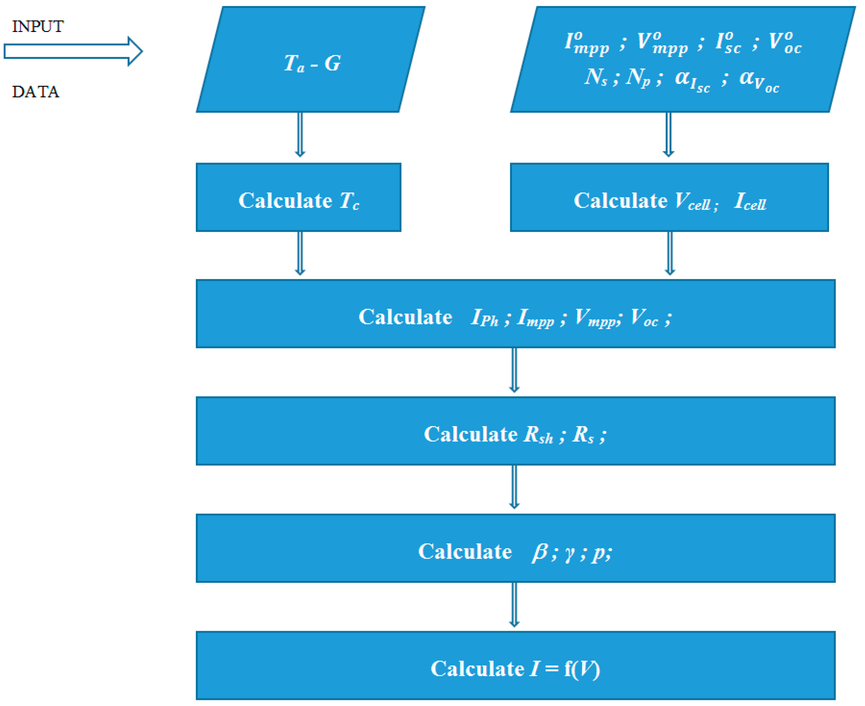
It results that the parameters β and γ depend on the ECs and on the manufacturers’ parameters. Finally, the mathematical model (12), together with Equations (15) and (16), allows tracing the I-V curve under variable ECs. Figure 3 shows a representative scheme to follow the several steps needed to calculate the final relationship between the current and the voltage for each point of the I-V curve under any ECs.

2.2. Mathematical Formulation of the Simplified Model

The resistor R_sh takes into account all the leakage current of the p-n junction depending on the fabrication process of the PV cell. Since its stronger influence is relevant in an uncommon region of operation, e.g., for low solar irradiation, then it can be neglected for higher irradiance value [20]. In this case, the resistor R_sh can be neglected [21,22] in the scheme of Figure 1 and the mathematical model results simplified. In fact, the Equations (12) and (14)–(16) become, respectively:

$$I=G_{pu}·\left(I_{sc}^o+{\mathsf{\alpha }}_{I_{sc}}·\Delta T\right)-\mathsf{\beta }·e^{\mathsf{\gamma }·\left(V+{\mathsf{\alpha }}_{V_{oc}}·\Delta T-V_{oc}^o\right)}$$

(17)

$$I_{sc}=G_{pu}·\left(I_{sc}^o+{\mathsf{\alpha }}_{I_{sc}}·\Delta T\right)$$

(18)

$$\mathsf{\beta }=G_{pu}·\left(I_{sc}^o+{\mathsf{\alpha }}_{I_{sc}}·\Delta T\right)$$

(19)

$$\mathsf{\gamma }=\frac{1}{V_{mpp}^o-V_{oc}^o}·log\frac{I_{sc}^o-I_{mpp}^o}{I_{sc}^o+{\mathsf{\alpha }}_{I_{sc}}·\Delta T}$$

(20)

and p = 1. Now, the logical scheme of Figure 3 is still valid, but the calculations are reduced, because R_sh is neglected.

3. Lumped Electrical Circuits

The mathematical models just defined can be implemented in any software or in a simple spreadsheet such as MATLAB, Mathematica, Microsoft Office-based suites, and so on. Nevertheless, several times one needs to study the time-domain behavior of the PV cell while the ECs change. Moreover, sometimes it is necessary to study the interaction between the PV cell/module and the other components directly linked to the PV cell/module or the interaction with the grid, if a grid-connected PV system is under study. In all these cases the circuit simulation is very effective because allows to monitor and display all the electrical variables in all possible ECs and OCs. This last feature is not always possible with other mathematical PV cell/module models, because they often require, for each EC, an iterative procedure to calculate internal parameters and this is a decisive obstacle for the implementation in a circuit simulation.

Instead, the proposed models (12) and (17) do not require iterative calculation for each EC, thus they can be easily implemented in the circuit simulators, where the solar radiance can be modelled as a variable resistor and the cell temperature as a voltage source.

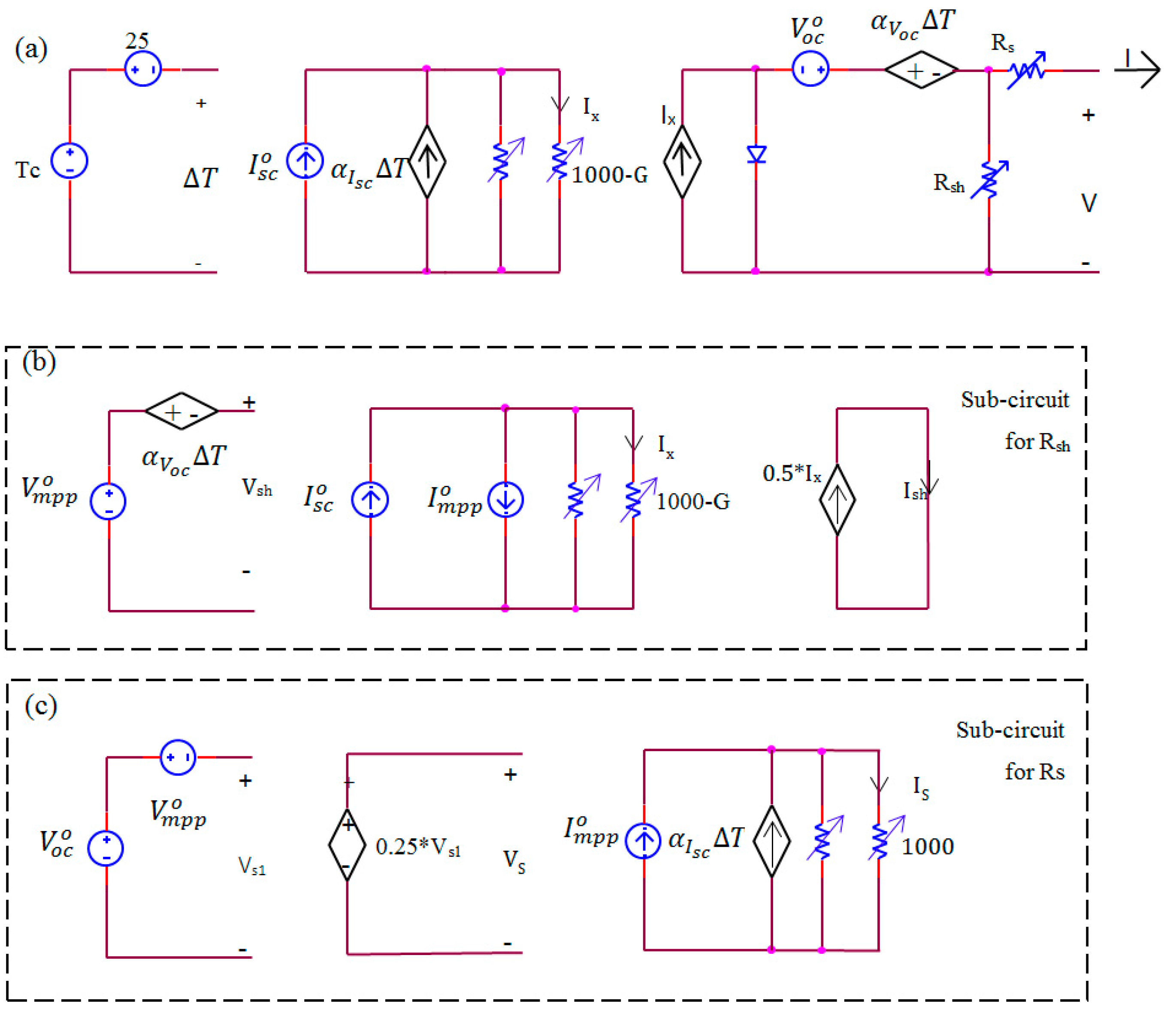
Figure 4 represents the electrical circuit of the complete model of the PV cell under arbitrary ECs. The mismatch ΔT = (T_c − 25) is modelled with two series-connected voltage sources; ΔT is the control variable of four voltage-controlled sources, which upgrade both $I_{sc}^o$ and $I_{mpp}^o$ by means of the coefficient ${\mathsf{\alpha }}_{I_{sc}}$ and both $V_{oc}^o$ and $V_{mpp}^o$ by means of the coefficient ${\mathsf{\alpha }}_{V_{oc}}$, respectively. The value G of the resistance is equal to the solar radiance, whereas the (1000 − G) resistance is the complementary value with respect to the solar radiance of 1000 W/m² stated in STC.

The first block of Figure 4a models the temperature mismatch (T_c − 25) the second block models the term $I_x=G_{pu}·\left(I_{sc}^o+{\mathsf{\alpha }}_{I_{sc}}·\Delta T\right)=\frac{G}{G+\left(1000-G\right)}·\left(I_{sc}^o+{\mathsf{\alpha }}_{I_{sc}}·\Delta T\right)$ of the Equation (12) by means of a current divider, finally the third block models the last two terms of the Equation (12). Moreover, the variable values of the resistances R_sh and R_s are calculated by means of the other two sub-circuits (Figure 4b,c, respectively), derived from the circuital interpretation of the Equations (10) and (11), respectively. The denominator of Equation (10), except for the division for 2, can be again interpreted as a current divider of the total current $\left(I_{sc}^o-I_{mpp}^o\right)$, therefore the second sub-circuit allows to calculate the ratio $\frac{V_{sh}}{I_{sh}}$ just equal to the value R_sh. For analogy, also the denominator of the Equation (11) can be interpreted as a current divider of the total current $G_{pu}·\left(I_{mpp}^o+{\mathsf{\alpha }}_{I_{sc}}·\Delta T\right)$, then the third sub-circuit is useful to calculate the ratio $\frac{V_s}{I_s}$ just equal to the value R_s.

This complete electrical circuit models a PV cell, but can also represent a whole PV module by using Equations (3) and (4) or a larger PV system by using analogous equations which define the connection scheme. Moreover, Equations (3) and (4) are valid under the hypothesis that all the PV cells show the same I-V curve, but this is not always verified, because they can experiment performance variations, as explained later at the end of Section 3. In these cases, it is needed to model each single PV cell and to group: (a) the series-connected cells by means of the Kirchhoff’s Voltage Law (KVL) $V_{series}=\sum _{j=1}^{N_s}{V}_j$ , being $V_j$ the voltage of the j-th cell; (b) the parallel-connected cells by means of the Kirchhoff’s Current Law (KCL) $I_{parallel}=\sum _{k=1}^{N_p}{I}_k$, being $I_k$ the current of the k-th cell.

Nevertheless, several circuits of Figure 4 can be connected each other, if we are interested in studying the interaction among two or more PV cells/modules under variable ECs and OCs. Then, two cases are possible: (a) the ECs are unique for all the PV parts under test; (b) the ECs are different for different PV parts. In the first case, only one electrical circuit of Figure 4 can be considered, by using Equations (3) and (4) if necessary, in the second case one electrical circuit of Figure 4 is used for each group of PV cell operating under the same ECs.

If the simplified model is used, the electrical circuit of Figure 4 is still valid after removing the resistor R_sh from Figure 4a and the companion sub-circuit (Figure 4b). Moreover the parameters of the datasheet are usually affected by spreading. Sometimes the spreading is balanced with respect to the rated value (e.g., ±X%), but other times not (e.g., (0, X%)). Both of the spreading typologies can be easily taken into account with the proposed model, considering a parametric simulation, which allows one to run several continuous simulations, including the extreme spreading values, in order to trace the whole real operation “area” of the PV module rather than a simple I-V curve.

4. Simulation Results and Discussion

The electrical circuit has been implemented in Spice environment and simulations have been run with a variable resistive load connected to the external pins. Nevertheless, since the circuit of Figure 4 is constituted by basic components and no devoted library is needed, the proposed models can be implemented in any circuit simulator. Three simulations have been run for the same mono-silicon PV module (whose datasheet parameters are reported in

Table 1. Electrical parameters at standard test conditions (STCs) (except for NOCT).

Material Technology	Pn (W)	VOC,STC (V)	ISC,STC (A)	VMPP (V)	IMPP (I)	NOCT (°C)	${\alpha }_{I_{sc}}$ (%/°C)	${\alpha }_{V_{oc}}$ (%/°C)
Mono-Si	180 ± 5	45% ± 3%	5.25% ± 3%	36.8	4.87	48 ± 2	0.1	−0.37

Mono-Si, mono-silicon; NOCT, nominal operating condition temperature.

) in three different ECs: under STCs (First), at high air temperature and STC solar radiance (Second), at high air temperature and low solar radiance (Third).

Table 2. Calculated values of the photo-voltaic (PV) module in Table 1.

Simulation	Ta (°C)	G (W/m2)	γ (V−1)	β (A)	Rsh (Ω)	Rs (Ω)
First (STCs)	25	1000	0.267	5.017	193.684	0.429
Second	40	1000	0.3234	5.093	180.540	0.414
Third	40	400	0.3282	2.037	451.390	2.589

STCs, standard test conditions.

presents the values of the three ECs and the values of the parameters calculated with the proposed method.

4.1. First Simulation

Figure 5 diagrams the results of the “First” simulation: a comparison between the I-V curve (solid blue line) derived from the Equation (12) and the datasheet I-V curve (dotted red line).

Instead, Figure 6 plots a comparison of the corresponding power-voltage (P-V) curves. Both Figure 5 and Figure 6 show good agreement between the simulated curves of the proposed model and the expected curves, as stated in the datasheet. Appreciable, but limited, difference is visible only at MPP.

4.2. Second Simulation

Figure 7 reports the comparison between the I-V curve derived from the proposed model (solid blue line) and the corresponding one of the datasheet (dotted red line) for the “Second” simulation (Table 2). Figure 8, instead, is the comparison between the PV-curves, respectively. As it can be seen, also in this case there is a light mismatch only in the MPP.

4.3. Third Simulation

Finally, Figure 9 reports the comparison between the I-V curves of the “Third” simulation (Table 2), whereas Figure 10 is the comparison between the PV-curves, respectively. As it can be seen, also in this case there is a light mismatch only in the MPP.

5. Conclusions

This paper has proposed a complete mathematical model of a PV cell, which can be easily extended to a PV module or to string or to a plant taking into account the connection scheme. The proposed model has three advantages: (a) it depends only on the parameters available in the manufacturer datasheet; (b) it is adaptive with respect to variable ECs; (c) it can be easily implemented in any circuit simulator, because the descriptive equation can be interpreted as an electrical circuit constituted by only basic analog electrical components and no devoted library is used. The model has been implemented in a Spice-based environment and the simulated curves match the expected ones. The differences resulting at the MPP in the Figure 6, Figure 7, Figure 8, Figure 9 and Figure 10 are due, first of all, on the fact that the proposed model is derived from the scheme of Figure 1 that is an approximated model of a real PV module. Moreover, a secondary reason depends on the parameter γ, whose value is strongly dependent on the constraint $\frac{dP}{dV}=0$ in MPP, where higher is the difference between the two curves. In any case, after running a lot of simulations under different ECs and for different PV modules, the maximum spread is always below the 2% of the maximum power under the ECs of the simulation. The losses usually modelled by two resistances (R_sh and R_s) have been taken into consideration. Finally, it has been proposed also a simplified model (neglecting R_sh), useful when specific conditions are verified.

References

1. Vergura, S.; Natangelo, E. Labview interface for data analysis of PV plants. In Proceedings of the International Conference on Clean Electrical Power (IEEE-ICCEP), Capri, Italy, 9–11 June 2009; pp. 236–241.
2. Sauer, K.J.; Roessler, T. Systematic approaches to ensure correct representation of measured multi-irradiance module performance in PV system energy production forecasting software programs. IEEE J. Photovolt. 2013. [Google Scholar] [CrossRef]
3. Manganiello, P.; Ricco, M.; Petrone, G.; Monmasson, E.; Spagnuolo, G. Optimization of perturbative PV MPPT methods through online system identification. IEEE Trans. Ind. Electron. 2014, 61, 6812–6821. [Google Scholar] [CrossRef]
4. Acciani, G.; Falcone, O.; Vergura, S. Typical defects of PV-cells. In Proceedings of the International Symposium on Industrial Electronics (IEEE-ISIE), Bari, Italy, 4–7 July 2010; pp. 2745–2749.
5. Vergura, S.; Acciani, G.; Falcone, O. A finite element approach to analyze the thermal effect of defects on silicon-based PV cells. IEEE Trans. Ind. Electron. 2012, 59, 3860–3867. [Google Scholar] [CrossRef]
6. Vergura, S.; Acciani, G.; Falcone, O. Modeling defects of PV-cells by means of FEM. In Proceedings of the International Conference on Clean Electrical Power (IEEE-ICCEP), Capri, Italy, 9–11 June 2009; pp. 52–56.
7. Vergura, S.; Acciani, G.; Falcone, O. 3-D PV-cell model by means of FEM. In Proceedings of the International Conference on Clean Electrical Power (IEEE-ICCEP), Capri, Italy, 9–11 June 2009; pp. 35–40.
8. Mahmoud, Y.; Xiao, W.; Zeineldin, H.H. A parameterization approach for enhancing PV model accuracy. IEEE Trans. Ind. Electron. 2013, 60, 5708–5716. [Google Scholar] [CrossRef]
9. King, D.L.; Boyson, W.E.; Kratochvill, J.A. Photovoltaic Array Performance Model, SANDIA Report. Available online: http://prod.sandia.gov/techlib/access-control.cgi/2004/043535.pdf (accessed on 2 March 2016).
10. Vergura, S.; Massi Pavan, A. On the PV explicit empirical model: Operations along the current-voltage curve. In Proceedings of the International Conference on Clean Electrical Power (IEEE-ICCEP), Taormina, Italy, 16–18 June 2015.
11. Cristaldi, L.; Faifer, M.; Leone, G.; Vergura, S. Reference string for statistical monitoring of photovoltaic fields. In Proceedings of the International Conference on Clean Electrical Power (IEEE-ICCEP), Taormina, Italy, 16–18 June 2015.
12. Lo Brano, V.; Orioli, A.; Ciulla, G.; di Gangi, A. An improved five-parameter model for photovoltaic modules. Sol. Energy Mater. Sol. Cells 2010, 94, 1358–1370. [Google Scholar] [CrossRef]
13. Tiana, H.; Mancilla-Davida, F.; Ellisd, K.; Muljadic, E.; Jenkinsd, P. A cell-to-module-to-array detailed model for photovoltaic panels. Sol. Energy 2012, 86, 2695–2706. [Google Scholar] [CrossRef]
14. Wu, X.; Bliss, M.; Sinha, A.; Betts, T.R.; Gupta, R.; Gottschalg, R. Accelerated spatially resolved electrical simulation of photovoltaic devices using photovoltaic-oriented nodal analysis. IEEE Trans. Electron. Devices 2015, 62, 1390–1398. [Google Scholar]
15. Townsend, T.U. A Method for Estimating the Long-Term Performance of Direct-Coupled Photovoltaic Systems. Master’s Thesis, University of Wisconsin-Madison, Madison, WI, USA, 1989. [Google Scholar]
16. Singh, P.; Ravindra, N.M. Temperature dependence of solar cell performance—An analysis. Sol. Energy Mater. Sol. Cells 2012, 101, 36–45. [Google Scholar] [CrossRef]
17. Markvart, T.; Castaner, L. Practical Handbook of Photovoltaics. Fundamentals and Applications; Elsevier: Oxford, UK, 2006. [Google Scholar]
18. Luque, A.; Hegedus, S. Handbook of Photovoltaic Science and Engineering; John Wiley and Sons: Chichester, UK, 2003. [Google Scholar]
19. Vergura, S. Scalable model of PV cell in variable environment condition based on the manufacturer datasheet for circuit simulation. In Proceedings of the Environment and Electrical Engineering International Conference on (IEEE-EEEIC 2015), Roma, Italy, 10–13 June 2015.
20. Di Piazza, M.C.; Vitale, G. Photovoltaic Sources: Modelling and Emulation; Springer: London, UK, 2013. [Google Scholar]
21. Cannizzaro, S.; di Piazza, M.C.; Luna, M.; Vitale, G. Generalized classification of PV modules by simplified single-diode models. In Proceedings of the International Symposium on Industrial Electronics (IEEE-ISIE), Istanbul, Turkey, 1–4 June 2014.
22. Cannizzaro, S.; di Piazza, M.C.; Luna, M.; Vitale, G. PVID: An interactive MATLAB application for parameter identification of complete and simplified single-diode PV models. In Proceedings of the 15th Workshop on Control and Modelling for Power Electronics (IEEE-COMPEL), Santander, Spain, 22–25 June 2014.
Figure 1. Five-parameters model of a photo-voltaic (PV) cell.
Energies 09 00326 g001
Figure 2. Current-voltage (I-V) curve for a typical photo-voltaic (PV) module.
Energies 09 00326 g002
Figure 3. Calculation scheme to get the relationship between current and voltage of a photo-voltaic (PV) cell.
Energies 09 00326 g003
Figure 4. Electrical circuit of a photo-voltaic (PV) cell, depending on the environmental conditions. (a) Main circuit; (b) Sub-circuiti for Rsh; (c) Sub-circuiti for Rs. Resistor Rsh and sub-circuit (b) are neglected for the simplified model.
Energies 09 00326 g004
Figure 5. Current-voltage (I-V) curve for the photo-voltaic (PV) module of Table 1 in standard test conditions (STCs). I-V curve of the proposed model (solid blue line) and I-V curve of the datasheet (dotted red line).
Energies 09 00326 g005
Figure 6. Power-voltage (P-V) curve for the photo-voltaic (PV) module of Table 1 in standard test conditions (STCs). P-V curve of the proposed model (solid blue line) and P-V curve of the datasheet (dotted red line).
Energies 09 00326 g006
Figure 7. Current-voltage (I-V) curve for the photo-voltaic (PV) module of Table 1 in environmental conditions (ECs) “Second” of Table 2. I-V curve of the proposed model (solid line) and I-V curve of the datasheet (dotted line).
Energies 09 00326 g007
Figure 8. Power-voltage (P-V) curve for the photo-voltaic (PV) module of Table 1 in environmental conditions (ECs) “Second” of Table 2. I-V curve of the proposed model (solid line) and I-V curve of the datasheet (dotted line).
Energies 09 00326 g008
Figure 9. Current-voltage (I-V) curve for the photo-voltaic (PV) module of Table 1 in environmental conditions (ECs) “Third” of the Table 2. I-V curve of the proposed model (solid line) and I-V curve of the datasheet (dotted line).
Energies 09 00326 g009
Figure 10. Power-voltage (P-V) curve for the photo-voltaic (PV) module of Table 1 in environmental conditions (ECs) “Third” of Table 2. I-V curve of the proposed model (solid line) and I-V curve of the datasheet (dotted line).
Energies 09 00326 g010