Abstract
Data from phasor measurement units (PMUs) may be exploited to provide steady state information to the applications which require it. As PMU measurements may contain errors and missing data, the paper presents the application of a Kalman Filter technique for real-time data processing. PMU data captures the power system’s response at different time-scales, which are generated by different types of power system events; the presented Kalman Filter methods have been applied to extract the steady state components of PMU measurements that can be fed to steady state applications. Two KF-based methods have been proposed, i.e., a windowing-based KF method and “the modified KF”. Both methods are capable of reducing noise, compensating for missing data and filtering outliers from input PMU signals. A comparison of proposed methods has been carried out using the PMU data generated from a hardware-in-the-loop (HIL) experimental setup. In addition, a performance analysis of the proposed methods is performed using an evaluation metric.
1. Introduction
1.1. Motivation
Funded by the European Commission’s 7th Framework Programme for Research and Technological Development program (FP7), the Ideal Grid for All (IDE4L) project has started to define, develop and demonstrate a distribution network automation system, IT systems and applications for active network management [1]. The project is composed of several work packages to cover different aspects of active network management. As part of work package 6 of the project, intelligent applications for monitoring, control and protection of active distribution networks are being developed by exploiting PMU data. As required by IEEE standards [2] the total vector error (TVE) between a measured phasor and its reference value should be less than 1% under steady state operation. However, in field installations, this criterion is not met due to the presence of different measurement uncertainties in PMU data [3]. Bad PMU data can distort Wide Area Monitoring System (WAMS) displays, jam calculation engines, or cause false alarms [4]. Therefore there is a clear need to process PMU data before using it in different applications. In [4,5,6] some methods of correcting different types of errors in PMU measurement are presented.
PMU measurements are polluted with noise, outliers, and missing samples. Thus, they cannot be directly fed to an application without adequate processing. Moreover, measurements obtained from PMUs during different events in power systems contain different signal features at different time scales. Hence they contain features of different types of power system dynamics. Not all PMU applications need the same type of signal. For steady state applications, the presence of oscillations adversly impacts the performance of the application [7]. Therefore, both bad data and oscillations should be filtered out from the PMU measurements before they can be fed to this kind of applications.
1.2. Literature Review
The application of Kalman filters (KFs) in state estimation using PMU data has been extensively discussed in [7,8,9,10]. In [7] a method for extracting the steady state of input PMU data using finite impulse response (FIR) and median filters was presented. However, important aspects of dealing with noise, outliers and replacing missing data from PMU measurements are not considered. Furthermore, the method has been discussed only for offline applications.
In [8] a PMU data conditioning algorithm for the PMU data was implemented using Kalman filters. In [9], an optimal assessment of the process noise covariance matrix Q on the accuracy of state estimation is made. A two-stage KF approach is presented in [10] to simultaneously estimate the static and dynamic states. In [11], a procedure is presented using iterated KF performing state estimation of an active distribution network by utilizing PMU measurements. In [12,13,14] dynamic state estimation for synchronous machines are presented using Extended KF (EKF) utilizing PMU measurements. None of these approaches, presented in these works, focus on the steady state estimation and are not suitable to extract steady state components from input PMU data. Therefore, a method is required to perform both data processing and extraction of steady state components from input PMU data in real-time.
1.3. Paper Contributions
Previous works do not consider that different applications will only utilize information about a specific time-scale contained in PMU data. The novelty of this paper is to apply the KF technique to separate the different time-scales. The paper presents the application of a KF technique for PMU data processing in real-time. The KF presented herein extracts the quasi-steady state component in PMU measurements and feeds them to steady state applications.
Two methods using KFs have been presented in this paper. The first KF method applies windowing of the PMU data; therefore it has limitations when utilized in the real-time applications. Therefore, a second KF method (i.e., “the modified KF”) is proposed, which is suitable for real-time applications as it does not perform windowing of PMU data.
The added value of proposed methods is to provide the “right” kind of information contained in the PMU data for the time-scale at which steady state applications (such as contingency analysis) or others operate. In addition, the methods are also capable of filtering noise, compensating for missing data and removing the outliers in PMU signals in real-time. The remainder of the paper is organized as follows: in Section 2, a general approach for PMU data processing is presented. Section 3 explains the traditional KFs. Section 4 describes the KF methods proposed in this paper in details. The HIL Lab Setup is presented in Section 5. Different case studies and comparison of proposed methods are presented in Section 6. Finally, Section 7 presents the key conclusions drawn in this paper.
2. PMU Data Processing
2.1. Extraction of Specific Signal Features
Figure 1 shows a signal containing the power system response to typical events, which leads to the dynamics at different time scales. Typical power system dynamic phenomenon that can be identified from different components of PMU signals are:
- Discrete Events (e.g., transmission line switching, transient stability) ~ milliseconds
- Small signal stability ~ seconds
- Tap changer operation (voltage stability) ~ minutes
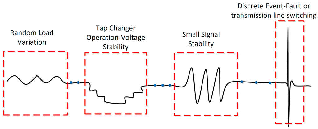
Figure 1.
Signal Features at different time scale in a PMU signal.
Identifying these events allows the system operator to take appropriate actions in time. Depending upon the nature of these events, actions can be preventive, corrective or restorative [15]. Therefore it is very important that the PMU applications that are used to identify these type of dynamic process are provided with ”clean” data so that no false actions can be taken based on an application’s results. The power system’s response to these events, captured by the PMU data, has to be processed in different ways before being fed to the applications (e.g., state estimation). So, the processing of PMU data should be application specific, i.e., the correct feature of the signal shown in Figure 1 should be extracted and fed to each application. The focus of this paper is steady state applications, so the raw PMU data is processed in an appropriate way in order to extract the steady state component from the signal.
2.2. Bad Data in PMU Measurements
Figure 2 shows a voltage magnitude as generated by a PMU using a hardware-in-the-loop (HIL) lab setup. Discrete events, such as, tap changer operation result in outliers in PMU data, as can be seen on the left hand side of Figure 2. These outliers can affect the performance of target applications. The other problem shown in Figure 2 is missing data. Missing data is not acceptable for many applications as calculations may be affected. Also shown in Figure 2 is the problem of measurement noise. Feeding noisy data to steady state applications can lead to wrong results. Therefore, all of these practical problems need to be addressed by using appropriate data processing methods. The data processing methods using KF, adopted in this paper to overcome these issues, will be discussed in the Section 4.
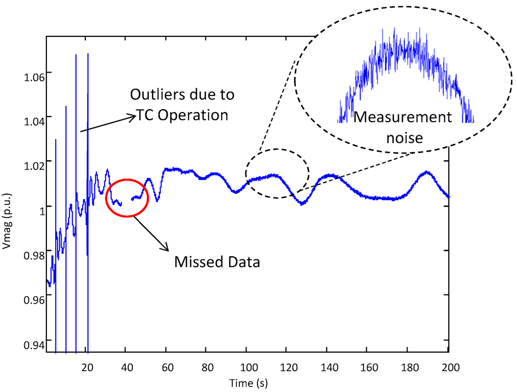
Figure 2.
Problems in PMU voltage measurement.
3. Traditional Kalman Filter
A linear discrete time controlled process is assumed to have linear stochastic process equations and measurement equations:
where x is the state vector, z is the measurement vector, A is the n × n matrix that relates the state at previous time step k−1 to the state at current step k, which is assumed to be constant in each iteration, B is the control input which relates input u to the state x and H is the m × n matrix which relates state xk to the measurements zk. The process noise ωk and measurement noise vk are assumed to be two mutually independent random variables with normal probably distributions:
where Q is the process noise covariance matrix and R is the measurement noise covariance matrix. These two matrices are usually constant but can be updated at each time step. The KF can be divided into two parts, as discussed below.
A. Time Update Equations (Prediction)
The time update equations are responsible of projecting forward (in time) the previous state and the error covariance estimate Pk–1 a priori state estimates and the a priori error covariance estimate for the next step k:
B. Measurements Update Equations (Correction)
Measurement update equations are responsible for feedback by incorporating a new measurement zk into the a priori estimate to obtain an improved a posteriori estimate:
where K is an n × m matrix known as Kalman gain matrix, zk is the actual measurement at step k, is the predicted measurement, is the a posteriori estimate which is a linear combination of an a priori estimate and a weighted difference between an actual measurement and predicted measurement. From the above expressions it can be concluded that as R approaches zero, an actual measurement zk is trusted more and predicted measurement is trusted less. On the other hand, as the a priori estimate error covariance approaches zero, the predicted measurement is trusted more than the actual measurement.
To summarize, the KF is a predictor-corrector algorithm. After each time and measurement update pair, the process is repeated with the previous a posteriori estimates used to project a new a priori estimate. In addition, the KF does not require all the previous data at each estimate, instead, it just recursively conditions the current estimate on all the past measurements. This makes the KF a suitable method for real time applications. Moreover, the accuracy of a Kalman Filter output is influenced by the measurement and process noise covariance matrices, i.e., R and Q [16]. Therefore these two parameters can be exploited in a proper way to perform bad data processing and also extracting the proper signal feature of the PMU data.
4. Proposed Kalman Filter Methods
In this paper, two different methods have been proposed to extract steady state components from input PMU data. The methods are explained in detail in the following subsections.
4.1. KF Method Based on Windowing
Originally introduced in [17], this proposed KF technique is implemented to extract the steady state components from PMU signals while removing all kinds of bad data from it. This is carried out by assuming that dynamic components in the PMU data are measurement noise. KF is applied to reduce the noise and increase the accuracy of PMU data by updating the value of R in each KF iteration. The KF algorithm was implemented in MATLAB. PMUs have a minimum of four state variables to be estimated, i.e., V, ϴ, I and δ which correspond to the variables that a PMU measures [18]. In the assumed process model given in Equation (1), i.e., A, is an identity matrix because the time step between KF iterations are small enough to assume that the current state is equal to the previous state, B is zero as there is no input to the process and H is also an identity matrix because the states are directly measured.
The overview of the KF implementation is shown in Figure 3. The initial estimates of xk−1 and Pk−1 are the input to the time update (prediction step). The predictor step is the same as given in Equation (3), projecting forward (in time) the previous state and error covariance estimate to produce the state and error covariance for the next step. The corrector step is, however, not the same as used in conventional KF. Instead, in addition to Equation (4), a residue is calculated in Equation (5) (for each sample) as the difference between state estimation and actual measurement zk:
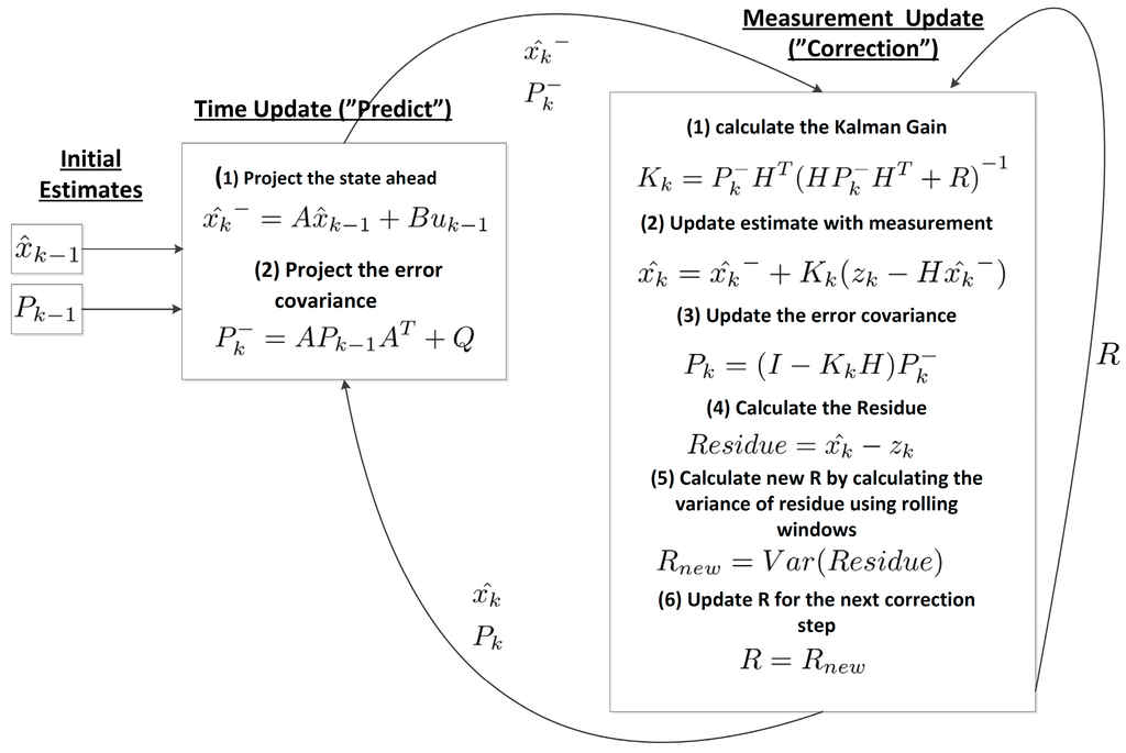
Figure 3.
Kalman filter windowing method overview.
The variance of the calculated residue in Equation (5) is computed in each step in Equation (6) using rolling windows. This gives the measurement covariance matrix R:
where E represents the mathematical expectation of the value. R is therefore updated in each time step, and is used in the start of next correction step:
As explained, instead of using a whole parcel of data at a time, the proposed method processes rolling windows of PMU data from which small signal oscillations and noise are filtered out. As can be inferred from the Equations, existence of any oscillation, noise or outlier leads to a large difference between the actual measurement zk and the state estimation , causing the residue to become larger. As R is calculated on the basis of the residue, R becomes larger as well. In this case the actual measurement zk is trusted less, while a priori state estimation is trusted more when calculating the new estimate . Therefore oscillations can be easily filtered out and a smoother response is obtained for steady state applications. It is worth noting that although the proposed KF method can be implemented in real-time, it’s not an optimum solution as it requires a window of data for calculation of the residue. Therefore, an improved KF method is developed which will be discussed next.
4.2. The Modified KF Method
R and Q can be updated in real-time to perform both bad data handling and extracting the steady state component of the PMU data. As we are only interested in the quasi-steady state component of the true state, any oscillations appearing in the measured signal will be identified and removed. R will be updated depending upon the quality of the measurements to filter out the bad data and extract the steady state component. Q will be updated to treat the unmodeled process noise which is, in our case, any change in the steady state value of the measured signal. This is because the process model, A, is set to the unity matrix, I, in order to force the output of the KF to settle at its steady state value.
The starting point of the proposed method relies on the concepts of Innovation (Inov) and Residue (Ires), mentioned in [10], in order to detect and differentiate between the bad data and the process noise:
where Inov has a normal probability density function and covariance Sk referred as Innovation Covariance which is calculated as:
Note that the mean value of Inov is normally zero, however, during abnormal conditions (i.e., there exists noise or bad data in the measurements) the mean value can shift such that the normalized innovation, described in Equation (10), will exceed a predetermined threshold value, τQ:
Similarly, Ires has a normal probability density function and covariance Tk referred to as Residual Covariance that can be calculated as:
Again, the mean value of Ires is normally zero, however in the presence of bad data, the mean value can shift such that the normalized residue, described in Equation (12), will exceed a pre-determined threshold value, τR. Note that the process noise does not affect Ires-norm. It is also worth noting that, in contrast to [10], we are using two separate threshold values for Inov-norm and Ires-norm in order to have a degree of freedom in differentiating between the process noise and the bad data:
For simplicity the time step k will be omitted from now on. Note that as a general rule, in KF methods, inflating Q leads to less dependence on the process model, i.e., matrix A, and inflating R leads to less dependence on the measurements.
Algorithm:
Figure 4 shows the flowchart of the proposed algorithm. Different steps of the algorithm are elaborated below:
- Start the prediction step. Afterwards, calculate Inov-norm. If Inov-norm ≥ tQ, it indicates that there exists either process noise or bad data in the measurements that has caused Inov-norm to exceed τQ. Assume that the problem is originating from the process noise, so reduce Inov-norm back to τQ through inflating Q by ΔQ, as shown in Equations (13)–(15).
- In this step, calculate Ires-norm considering the inflated Q. If Ires-norm < tR, it means that the assumption in step 2 is correct, otherwise it indicates that the problem is caused by the bad data in the measurements. So this requires to deflate Q back to its original value and instead, inflate R such that Inov-norm and Ires-norm are reduced back to τQ (through Equations (16) and (17)) and τR (through Equations (18) and (19)), respectively. Note that as Equation (19) is a nonlinear equation, it must be solved numerically, e.g., R2 can be increased iteratively starting from R until R2(cte+R2)–1 ≥ T2. Finally note that, as shown in Equation (20), the inflated R is equal to the maximum of R1 and R2.
- The correction step is performed using the inflated Q or R. If neither Q nor R is inflated, the method uses the original Q and R.
- The inflated Q or R is deflated using an exponential decaying factor in the beginning of the next execution to treat temporary problems, e.g., outliers, etc.
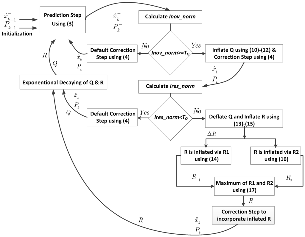
Figure 4.
The Modified KF Method overview.
As explained, the improved KF processes only one data at a time which makes it suitable for real-time implementation.
5. Experimental Setup
This section describes the HIL real-time simulation setup in which the KF methods developed in the previous sections, are validated. As shown in Figure 5, two measurement locations have been specified on a grid model [19] that is simulated using the OPAL-RT Technologies real-time simulator [20]. The measured voltages and currents are fed to PMUs through the analogue output ports of the OPAL-RT simulator.
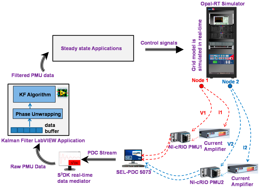
Figure 5.
Hardware-in-the-Loop (HIL) Lab Setup.
As indicated in the figure, the PMUs used in this setup are Compact Reconfigurable IO systems (cRIO) from National Instruments Corporation [21], programmed with LabVIEW graphical programming tools to perform phasor calculations [22]. As the figure shows, the current signals are passed through the current amplifiers by Megger [23] before being fed to the PMUs. Syncrophasors are then sent to a Phasor Data Concentrator (PDC) which streams the data over TCP/IP to a workstation computer holding Statnett’s Synchrophasor Development Kit (S3DK) [24], the real-time data mediator that parses the PDC data stream and makes it available to KF application in the LabVIEW environment. The output of the KF application is stored in a reconfigurable data buffer, from which the steady state applications read the data.
6. Case Studies
6.1. Difference Between Simulated Data and PMU Data
PMU application development cannot rely on offline simulation data only. There are many practical issues that can be observed from real PMUs that are not present in offline simulations. For example, Figure 6 shows a very clear illustration for this argument. A power system is disturbed with random load variations (RLV) activated at t = 45 s and deactivated at t = 115 s. The voltage response from the simulation and the HIL PMU setup is shown in Figure 6. It can be clearly seen that the voltage from the HIL PMU setup has missing data, which is due to the fact that the PMU data is delayed for a longer time than the PDC maximum waiting time. Also, with the discrete event of connection and disconnection of the RLV, the PMU generates outliers. Hence, in the development of methods in Section 4 and the illustrations below, only data from the RT HIL setup is used.
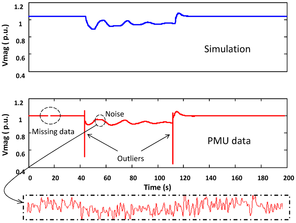
Figure 6.
Difference between voltage responses from simulation and an actual PMU for the same disturbance.
6.2. Kalman Filter Performance Comparison of Two Proposed Methods
The developed KF methods are applied on HIL PMU data. A power system is disturbed with RLV activated at t = 5 s and deactivated at t = 75 s. The performances of both methods proposed in Section 4 are compared. Figure 7 shows the KF algorithm performance for both methods for the PMU voltage magnitude signal. When the disturbance is applied at t = 5 s and removed at t = 75 s, outliers are generated in the PMU voltage signal. The RLV excites the small signal oscillations, which should be neglected in a steady state application. As the figure shows, by applying the proposed methods, the dynamics and outliers are filtered, giving smoother responses to be used in steady state applications. The response of “the modified KF” is better than the windowing method with a rolling window (RW) length of 0.5 s. In addition, the resulting responses of R are shown in Figure 8. It can be noticed from the figure that R increases for both methods in case of outliers in the data. However, for “the modified KF”, R comes back to its normal state much faster because it does not require data windowing. The response of the both KF method during normal operation of power system has also been shown in the right top of the Figure 7. It is worth noticing that both KF methods reduce the noise during the normal operation of the power system (no events). This increases the overall probability of the PMU data.
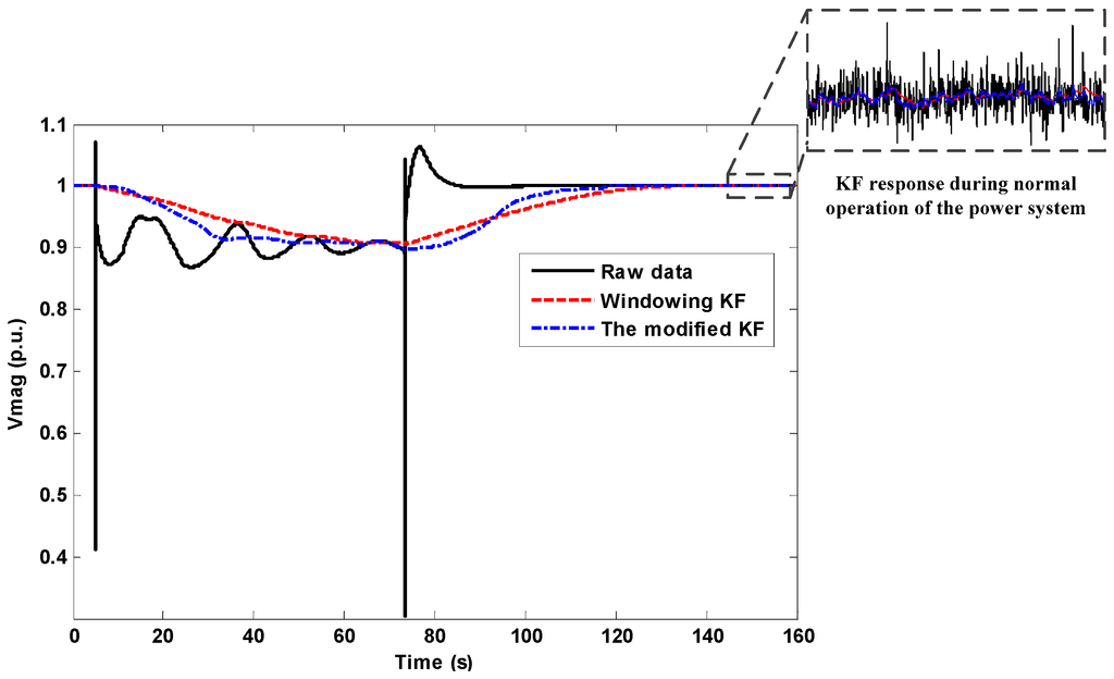
Figure 7.
Comparison of two proposed KF methods (for PMU’s voltage magnitude signal).
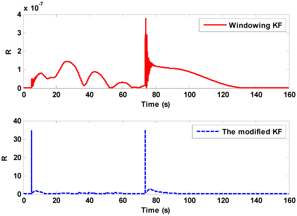
Figure 8.
Comparison for updating R for proposed KF methods (for voltage magnitude signal).
Figure 9 shows the application of the proposed methods for the PMU voltage angle signal. Similar to the voltage magnitude, RLV excites the small signal oscillations in PMU voltage angle signal. These dynamic components are removed from the voltage angle signal for both methods, by updating either R and/or Q in the correction step of the algorithm. Hence smoother estimation for the voltage angle is obtained as shown in Figure 9.
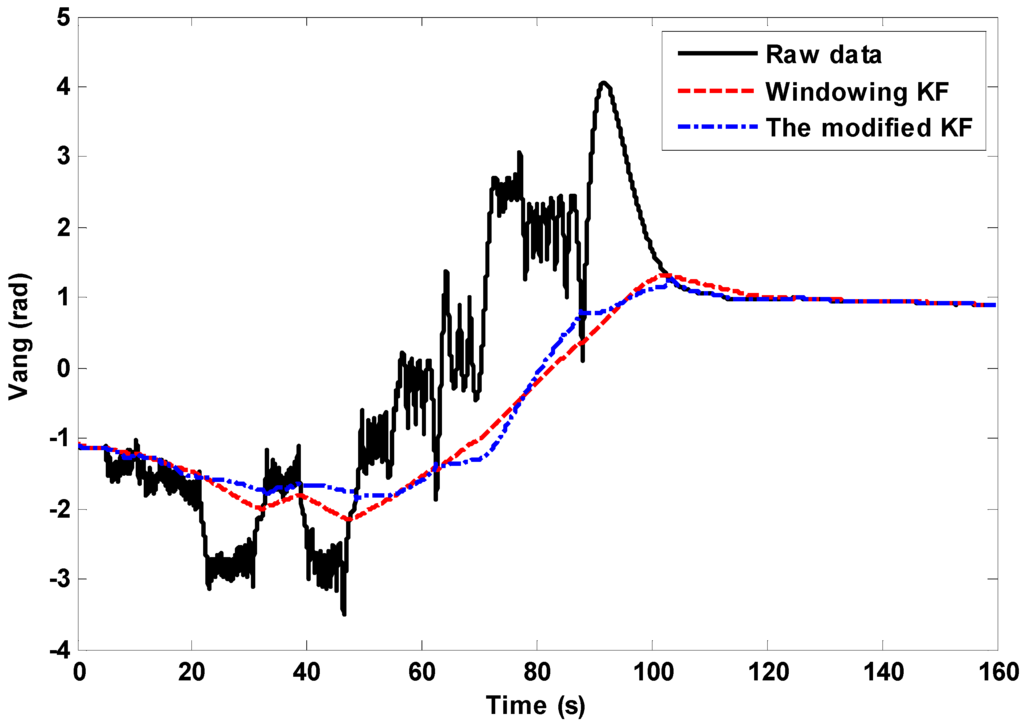
Figure 9.
Performance comparison of two proposed KF methods (for PMU’s voltage angle signal).
The resulting responses of R are shown in Figure 10. It is worth noticing that the responses of updating R are different in both methods based upon the fact that both methods used a different logic to update R. Although there are no outliers in voltage angle signal, R increases for both methods during the period having oscillations. For “the modified KF”, R comes back to its normal state much faster than with the windowing method.
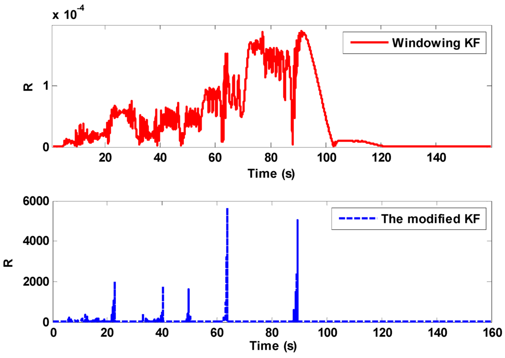
Figure 10.
Comparison for updating R for proposed KF methods (for voltage angle signal).
6.3. Performance Analysis
The performance of both methods is analyzed. The first method (as presented in the Section 4.1) uses data windowing; therefore the impact of changing the window length is first investigated. Secondly, an evaluation metric is introduced to quantify and compare the performance of both methods.
6.3.1. Impact of Varying Rolling Window Length on Smoothing
The size of the rolling window (RW) affects the smoothing of the states in the presence of outliers and oscillations. By varying the RW length, the updating of R varies, resulting in different responses for signal smoothing. Figure 11 shows different responses for the PMU voltage magnitude with different lengths of RW. For a length of RW = 0.5 s, a fast KF response is obtained together with a smoothed output which captures the exponential decay of the small signal oscillations. However, as soon as the RW length increases, the response of the KF becomes slower. For example the response for RW = 5 s is slow and it could not produce accurate smoothing. It can be thought of an over-filtered response. It can be concluded from the discussion above that a smaller RW length produces better smoothing and a faster response.
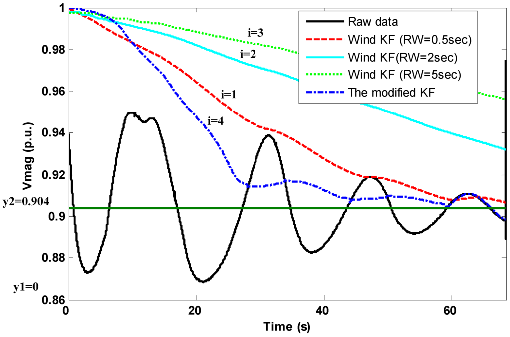
Figure 11.
Performance analysis for voltage magnitude signal.
6.3.2. Performance Analysis Using an Evaluation Metric
Table 1 shows the performance analysis of the KF windowing algorithm for different RW lengths and for “the modified KF”. The steady state value of the raw PMU data is assumed as the average value of the signal between the time period of t1 and t2, which comes out to be 0.904 p.u. (green line in Figure 11). The areas between the steady state value and each filtered signals are calculated as follows:
where f0 is a straight line at (t1, y2) and (t2, y2) and i = 1, 2 and 3 corresponding to the filtered signals with RW lengths of 0.5, 2 and 5 s, respectively and I = 4 for “the modified KF” (see Figure 11). The areas in Equation (21) are calculated by computing the integrals in MATLAB using the trapezoidal numerical integration “trapz” command.

Table 1.
Performance analysis using an evaluation metric (A/K).
The term A/K, where K is the base value for calculating the per unit area, represent the area’s value in per unit and is defined as the performance evaluation metric to compare the performance of proposed KF methods. It is also used to assess the performance of the first method (data windowing) with different lengths of rolling windows. As a general rule, a response having a small per united area (the value of A/K) should produce more accurate results (must follow the steady state value accurately).
The evaluation metric A/K has the highest value for windowing method for the case RW = 5 s and lowest for the case RW = 0.5 s. This means that RW = 5 is the worst in following the steady state value and RW = 0.5 has the best performance as can be seen from Figure 11. By comparing the performance of both methods (i.e., windowing method and “the modified KF”), the response for “the modified KF” has the minimum value of evaluation metric A/K showing that it performs better than windowing method.
7. Conclusions
The results in this paper show that the proposed methods using Kalman filters are suitable for processing PMU data to be fed to steady state applications. It has been shown that by updating the value of the measurement noise covariance matrix R in the windowing method, dynamics and bad data can be filtered out from raw PMU data. In the case of “the modified KF”, R will be updated depending upon the quality of the measurements to filter out the bad data and to extract steady state components. In addition, Q will be updated to treat the unmodeled process noise which is, in our case, any change in the steady state value of the measured signal. Although both of the proposed KF methods have been developed for real time implementation, “the modified KF” is more suitable for real time applications as it does not perform any data windowing. The performance comparison analysis shows that “the modified KF” has the best performance to follow the steady state when a disturbance is applied.
Acknowledgments
This work was supported in part by EU-funded Seventh Framework Programme for Research and Technological Development (FP7) Ideal Grid for All (IDE4L) Project, the STandUP for Energy Collaboration Initiative and by Statnett SF, the Norwegian Transmission System Operator.
Author Contributions
The corresponding author Farhan Mahmood performed the experiments and wrote the paper. The co-authors Hossein Hooshyar and Luigi Vanfretti designed the experiments and analyzed the results presented in this paper.
Conflicts of Interest
The authors declare no conflict of interest.
Abbreviations
The following abbreviations are used in this manuscript:
| KF | Kalman Filters |
| HIL | Hardware-in-the-Loop |
| CRIO | Compact Reconfigurable Input Output |
| RLV | Random Load Variations |
References
- IDE4L. Ideal Grid for All. Available online: http://www.ide4l.eu/ (accessed on 8 December 2015).
- Institute of Electrical and Electronics Engineers (IEEE). IEEE Standard for Syncrophasor Measurements for Power Systems; IEEE Std C37.118.1-2011; IEEE: New York, NY, USA, 2006. [Google Scholar]
- Almas, M.; Kilter, J.; Vanfretti, L. Experiences with steady-state PMU compliance testing using standard relay testing equipment. In Proceedings of the Electric Power Quality and Supply Reliability Conference (PQ) 2014, Rakvere, Estonia, 11–13 June 2014; IEEE: New York, NY, USA; pp. 103–110.
- Zhang, Q.; Luo, X.; Bertagnolli, D.; Maslennikov, S.; Nubile, B. PMU data validation at ISO New England. In Proceedings of the Power and Energy Society General Meeting (PES), Vancouver, BC, Canada, 21–25 July 2013; IEEE: New York, NY, USA, 2013; pp. 1–5. [Google Scholar]
- Shi, D.; Tylavsky, D.; Logic, N. An adaptive method for detection and correction of errors in PMU measurements. In Proceedings of the Power and Energy Society General Meeting (PES), Vancouver, BC, Canada, 21–25 July 2013; IEEE: New York, NY, USA, 2013; p. 1. [Google Scholar]
- Zhang, Q.F.; Venkatasubramanian, V.M. Synchrophasor time skew: Formulation, detection and correction. In Proceedings of the North American Power Symposium (NAPS), Pullman, WA, USA, 7–9 September 2014; pp. 1–6.
- Tate, J.; Overbye, T. Extracting steady state values from phasor measurement unit data using FIR and median filters. In Proceedings of the IEEE PES Power Systems Conference and Exposition, Seattle, WA, USA, 2009.
- Jones, K.D.; Pal, A.; Thorp, J.S. Methodology for performing synchrophasor data conditioning and validation. In IEEE Transactions on Power Systems; IEEE: New York, NY, USA, 2015; Volume 30, pp. 1121–1130. [Google Scholar]
- Zanni, L.; Sarri, S.; Pignati, M.; Cherkaoui, R.; Paolone, M. Prob-abilistic assessment of the process-noise covariance matrix of discrete kalman filter state estimation of active distribution networks. In Proceedings of the Inter-national Conference on Probabilistic Methods Applied to Power Systems (PMAPS), Durham, UK, 7–10 July 2014.
- Zhang, J.; Welch, G.; Bishop, G.; Huang, Z. A two-stage kalman filter approach for robust and real-time power system state estimation. IEEE Trans. Sustain. Energy 2014, 5, 629–636. [Google Scholar] [CrossRef]
- Sarri, S.; Paolone, M.; Cherkaoui, R.; Borghetti, A.; Napolitano, F.; Nucci, C.A. State estimation of Active Distribution Networks: Comparison between WLS and iterated kalman-filter algorithm integrating PMUs. In Proceedings of the 2012 3rd IEEE PES International Conference and Exhibition on Innovative Smart Grid Technologies (ISGT Europe), Berlin, Germany, 14–17 October 2012; pp. 1–8.
- Ghahremani, E.; Kamwa, I. Simultaneous state and input estimation of a synchronous machine using the Extended Kalman Filter with unknown inputs. In Proceedings of the 2011 IEEE International Electric Machines & Drives Conference (IEMDC), Niagara Falls, ON, Canada, 15–18 May 2011; pp. 1468–1473.
- Ghahremani, E.; Kamwa, I. PMU analytics for decentralized dynamic state estimation of power systems using the extended kalman filter with unknown inputs. In Proceedings of the 2015 IEEE Power & Energy Society General Meeting, Denver, CO, USA, 26–30 July 2015; pp. 1–5.
- Ghahremani, E.; Kamwa, I.; Li, W.; Grégoire, L.A. Synchrophasor based tracking of synchronous generator dynamic states using a fast EKF with unknown mechanical torque and field voltage. In Proceedings of the Industrial Electronics Society, IEEE International Conference on Industrial Electronics, Control, and Instrumentation (IECON) 2014—40th Annual Conference of the IEEE, Dallas, TX, USA, 29 October–1 November 2014; pp. 302–308.
- Giri, J.; Sun, D.; Avila-Rosales, R. Wanted: A more intelligent grid. Power Energy Mag. 2009, 7, 34–40. [Google Scholar] [CrossRef]
- Hongrae, K.; Abur, A. Enhancement of external system modeling for state estimation. IEEE Trans. Power Syst. 1996, 11, 1380–1386. [Google Scholar] [CrossRef]
- Mahmood, F.; Hooshyar, H.; Vanfretti, L. A method for extracting steady state components from Syncrophasor data using Kalman Filters. In Proceedings of the IEEE 15th International Conference on Environment and Electrical Engineering (EEEIC), Rome, Italy, 10–13 June 2015; pp. 1498–1503.
- Vanfretti, L.; Chow, J.; Sarawgi, S.; Fardanesh, B. Phasor data- based state estimator incorporating phase bias correction. IEEE Trans. Power Syst. 2011, 26, 111–119. [Google Scholar] [CrossRef]
- Hooshyar, H.; Mahmood, F.; Vanfretti, L.; Baudette, M. Specification, implementation, and hardware-in-the-loop real-time simulation of an active distribution grid. Sustain. Energy Grids Netw. 2015, 3, 36–51. [Google Scholar] [CrossRef]
- The Opal-RT Technologies, Inc. OP5600 Hardware-in-the-Loop (HIL) Simulator Description. Available online: http://www.opal-rt.com/product/op5600-hil-hardware-in-the-loop-computer-and-IO-system? quicktabs 3=7#quicktabs-3 (accessed on 6 January 2016).
- National Instruments. NI cRIO-9074 Description. Available online: http://sine.ni.com/nips/cds/view/p/lang/en/nid/203964 (accessed on 6 January 2016).
- Romano, P.; Paolone, M. Enhanced Interpolated-DFT for Synchrophasor Estimation in FPGAs: Theory, Implementation, and Validation of a PMU Prototype. IEEE Trans. Instrum. Meas. 2014, 63, 2824–2836. [Google Scholar] [CrossRef]
- Megger. Single Phase Relay Tester (SMRT1) Description. Available online: http://www.megger.com/us/products/ProductDetails.php?ID= 1529 (accessed on 6 January 2016).
- Vanfretti, L.; Aarstrand, V.H.; Almas, M.S.; Peric, V.S.; Gjerde, J.O. A software development toolkit for real-time synchrophasor applications. In Proceedings of the IEEE Power Tech, Grenoble, France, 16–20 June 2013.
© 2016 by the authors; licensee MDPI, Basel, Switzerland. This article is an open access article distributed under the terms and conditions of the Creative Commons Attribution (CC-BY) license (http://creativecommons.org/licenses/by/4.0/).