Article

Analysis of a Battery Management System (BMS) Control Strategy for Vibration Aged Nickel Manganese Cobalt Oxide (NMC) Lithium-Ion 18650 Battery Cells

1
Warwick Manufacturing Group (WMG), University of Warwick, Coventry CV4 7AL, UK
2
Jaguar Land Rover, Banbury Road, Warwick CV35 0XJ, UK
*
Author to whom correspondence should be addressed.
Energies 2016, 9(4), 255; https://doi.org/10.3390/en9040255
Submission received: 31 January 2016 / Revised: 26 February 2016 / Accepted: 21 March 2016 / Published: 1 April 2016
(This article belongs to the Special Issue Control of Energy Storage)

Abstract

:
Electric vehicle (EV) manufacturers are using cylindrical format cells as part of the vehicle’s rechargeable energy storage system (RESS). In a recent study focused at determining the ageing behavior of 2.2 Ah Nickel Manganese Cobalt Oxide (NMC) Lithium-Ion 18650 battery cells, significant increases in the ohmic resistance (RO) were observed post vibration testing. Typically a reduction in capacity was also noted. The vibration was representative of an automotive service life of 100,000 miles of European and North American customer operation. This paper presents a study which defines the effect that the change in electrical properties of vibration aged 18650 NMC cells can have on the control strategy employed by the battery management system (BMS) of a hybrid electric vehicle (HEV). It also proposes various cell balancing strategies to manage these changes in electrical properties. Subsequently this study recommends that EV manufacturers conduct vibration testing as part of their cell selection and development activities so that electrical ageing characteristics associated with road induced vibration phenomena are incorporated to ensure effective BMS and RESS performance throughout the life of the vehicle.

1. Introduction

Within the road transport sector, a main driver for technological innovation is the need to reduce fuel consumption and vehicle exhaust emissions. Legislative requirements are motivating original equipment manufacturers (OEMs) to develop and integrate new and innovative technologies into their fleet. Consequently, over the last few years, different types of electric vehicles (EVs) have been built alongside conventional internal combustion engine (ICE) cars. Within the field of EVs, a key enabling technology is the design and integration of rechargeable energy storage systems (RESS) [1,2]. Multi-cell RESSs require a battery management system (BMS) to ensure safe and consistent operation over the life of the vehicle and to report the status of the RESS to the wider vehicle control systems. One of the key challenges is to monitor the variations in capacity and impedance between cells. Often, the RESS is limited by characteristics of the weakest cell [3,4], and accounting for these differences minimizes the impact of cell variation on RESS performance.
Many OEMs are employing cylindrical format cells (e.g., 18650) for the design and construction of the RESS [5,6,7,8]. Cylindrical cells are often chosen in EV applications over their prismatic and pouch cell counterparts because of a combination of factors. For example, 18650 format cells are produced in very large quantity which makes them cost effective [8,9,10]. Similarly, they may have built-in safety systems such as a positive temperature coefficient (PTC) resistor that prevents high current surge and the use of a current interrupt device (CID) to protect the cell in the event of excessive internal pressure [8,9,10].
To ensure in-market reliability and customer satisfaction, OEMs perform a variety of life representative durability tests during the design and prototype stages of the development process. Firstly, these tests ensure that new vehicle sub-assemblies and components are fit-for-purpose. Secondly, it allows OEMs to obtain characterization data for models that are used for the development of core functionality within the BMS. Thirdly, it ensures that the product meets strict requirements for vehicle homologation.
Vibration durability is one of these tests, and plays an important role in the selection of components. As discussed within [11,12,13,14,15] poorly integrated components, assemblies or structures subjected to vibration can result in a significantly reduced service life or the occurrence of catastrophic structural failure through fatigue cracking or work hardening of materials [13,16,17].
With respect to 18650 format battery cells, vibration-induced degradation in cell electrical performance has been previously reported. In [18], 18650 format Li-ion cells, of unknown chemistry, were subjected to a vibration profile along the Z-axis of the cells. The cells were clamped to an electromagnetic shaker (EMS) table and excited for 186 h with a swept-sine wave from 4 to 20 Hz and back to 4 Hz in 30 s. The authors reported that most of the cells exhibited an increase in resistance along with a reduction in their 1C discharge capacity. Additionally, they described the occurrence of complete cell level failures, such as an internal short circuit. The latter failure mode was attributed within the research to the central mandrel becoming loose during the vibration test, which in turn damaged the upper and lower cell components, including the current collector and tabs.
In [19], commercially available nickel manganese cobalt oxide (NMC) Samsung 2.2 Ah 18650 cylindrical cells (model number ICR18650-22F) were evaluated for electrical degradation when subjected to vibration profiles representative of 100,000 miles of European and North American customer use for chassis mounted RESS. The two batches of cells were evaluated to two different random vibration cycles:
  • Society of Automotive Engineers (SAE) J2380 [20];
  • WMG/Millbrook Proving Ground (WMG/MBK) profiles [21,22].
Both batches of cells displayed a significant increase in ohmic resistance (RO) regardless of vibration profile utilized for their assessment. Increases in RO were within the range of 17.4% to 128.1%. A reduction in capacity was also observed in some samples evaluated, with 12.22% being the greatest reduction observed. It was acknowledged within [19] that the impact of vibration-induced ageing may require greater levels of cell balancing by the battery management system (BMS), when the cells are aggregated to form a rechargeable energy storage system (RESS). As a result, the authors are proposing to utilize the electrical data obtained from the vibration aged Samsung 18650 cells defined in [19] to determine, via simulation techniques, the specific impact on the BMS strategy of a hybrid electric vehicle (HEV) and plug-in hybrid electric vehicle (PHEV).
This paper is structured as follows: Section 2 of this paper provides a detailed overview of the experimental method employed to assess vibration-induced ageing. Section 3 summarizes the experimental results. The cell modelling techniques are introduced in Section 4 and the models are parameterized in Section 5. Two case studies, considering the impact of vibration-aged cells in series and parallel connections, are presented in Section 6, using the models parameterized from the experimental data. Further work and conclusions are presented in Section 7 and Section 8, respectively.

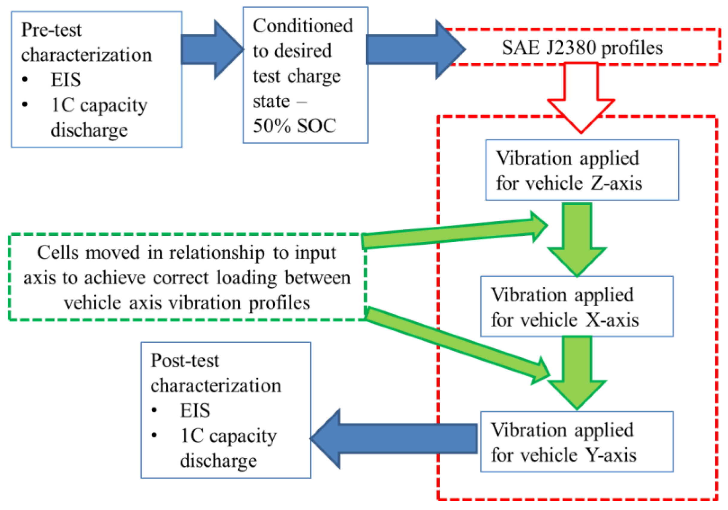
2. Experimental Method—Vibration Ageing of Cells

The following section is a summary of the experimental method employed for the vibration ageing of the cells, whose electrical data is used to parameterize the cell models. Additional information with respect to the test fixtures, facility, instrumentation and sample arrangement are defined in [19]. Note that only samples evaluated to the SAE J2380 standard, and assessed at 50% SOC in [19] are employed within this study. The experimental procedure followed during this test programme is summarized in Figure 1.

2.1. Test Samples

Table 1 defines the details of sample preparation, cell SOC and cell orientation of five Samsung 2.2 Ah 18650 cells (NMC). Three samples were subject to vibration in accordance to SAE J2380, whilst the remaining two were defined as control cells. The control samples were not subjected to any vibration loading [19]. During testing, the control samples were either co-located within the same environmental conditions as the test cells or kept in permanent storage.

2.2. Pre-test Characterization

The five cells presented in Table 1 were electrically characterized as described in the remainder of this section. Additional information on the cell electrical characterization methods are discussed in [19]. It must be noted that other electrical characterization tests were conducted on these cells, however only the characterization tests relating to the data required for cell modelling are described within this Section (and illustrated by Figure 1).

2.2.1. Electrochemical Impedance Spectroscopy (EIS)

EIS data was recorded 4 h after the last pulse of the pulse power tests, as suggested by Barai et al. [23] and was performed at 50% SOC. The EIS measurement was carried out in a galvanostatic mode using a ModuLab® (Solartron, Leicester, UK) electrochemical system model 2100 A fitted with a 2 A booster and driven by Modulab® ECS software. The EIS spectra were collected within the frequency range of 10 mHz to 10 kHz using 10 frequency points per decade. The amplitude of the applied current was 200 mA (RMS). No DC current was superimposed on the RMS value.

2.2.2. 1 C Capacity Discharge

The cells were fully charged using a constant current phase of 1.1 A (C/2) to 4.2 V followed by a constant voltage phase at 4.2 V until the current reduced to 0.05 A (C/44). The cells were allowed to rest for 4 h prior to being fully discharged at 1 C to 2.75 V, which is the lower voltage threshold as defined by the manufacturer. The charge extracted from the cells during the discharge was recorded as a measure of the 1 C capacity.

2.3. Conditioning to Desired Test Charge State

Following electrical characterization, each cell was pre-conditioned to a defined SOC (either 25% 50% or 75% SOC) prior to durability testing and allocated a test orientation with respect to the vehicle Z-axis (discussed further in Section 2.4). The cell SOC was adjusted by fully charging the cells with a constant current of 1.1 A (C/2) to 4.2 V followed by a constant voltage phase at 4.2 V until the current fell to 0.05 A (C/44). At the end of charge, the cells were allowed to rest for 4 hours prior to being discharged at 1 C for 30 min, to achieve a cell SOC of 50%. The cells were allowed to relax for 4 h before the application of vibration energy.

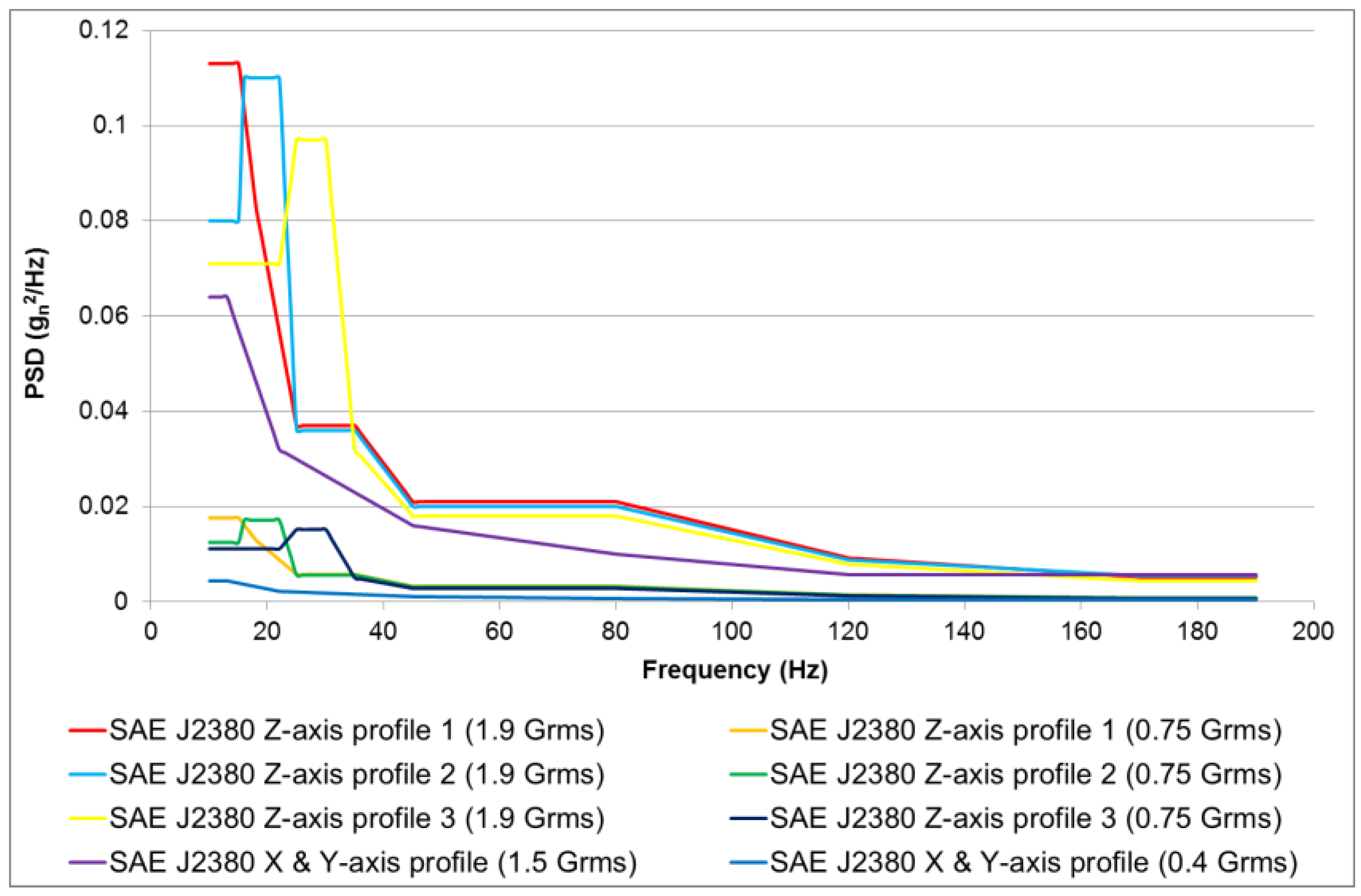
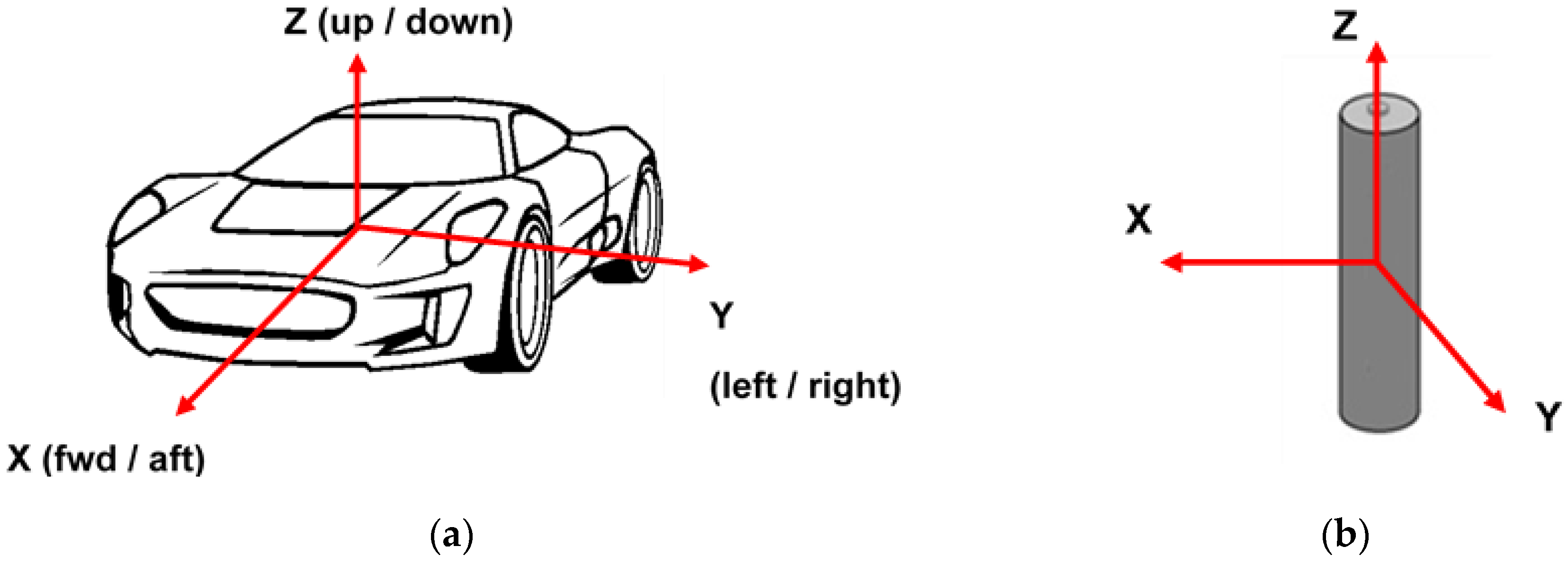
2.4. Application of SAE J2380 Vibration Profiles and Cell Orientation

SAE J2380 was selected as the desired vibration durability method. The SAE J2380 profiles are presented in Figure 2.
SAE J2380 is currently the only internationally recognized vibration test standard that has been correlated to 100,000 miles of road vehicle durability (North American vehicle usage by the 90 percentile customer) [20,21,22], and has been devised to assess multiple types of chassis mounted RESS (and their associated sub components). Unlike traditional vibration standards (such as UN38.3 Test 3) which have been devised to assess the fail-safe performance of EV batteries when subjected to extreme vibration conditions (such as during shipment via air or during a vehicle to vehicle crash) SAE J2380 has been synthesized from “road induced vibration excitation” associated with normal customer usage. This specification applies vibration loading through a “random” excitation which is more representative of road-induced structural vibration than contemporary vibration specifications [13]. Also unlike other EV standards (such as UN38.3 Test 3 or ECE R100) SAE J2380 applies vibration to each cell in the X, Y and Z axis, as opposed to applying vibration in a single axis for the duration of the test [1,21,22]. It is beyond the scope of this paper to discuss in detail the derivation of the vibration profiles. However, this information is discussed within [13,21,22,24,25].
As part of the experimental procedure, each profile is sequentially applied to the cells to achieve the desired 100,000 miles of representative EV life. For a complete execution of SAE J2380 the three different combinations of vibration loads with respect to each cell orientation are defined below:
  • Z:Z to X:X to Y:Y
  • Z:X to X:Y to Y:Z
  • Z:Y to X:Z to Y:X
Using the above notation, for each pair of letters, the first letter refers to the vehicle axis, whilst the second refers to cell orientation. For simplicity this paper identifies the cell orientation in relationship to the vertical (Z axis) of the vehicle. For example a cell that was subject to the vibration sequence of Z:X to X:Y to Y:Z, is referred to as being evaluated in the Z:X orientation. Figure 3a illustrates the axis convention for the vehicle axis, whilst Figure 3b illustrates the axis convention for the 18650 cell.
Due to limited equipment availability, a single axis Derriton (Hastings, UK; model number: VP85, serial number: 74) shaker was employed for the durability testing. Because the orientation of the EMS could not be changed, the cells had to be rotated on the durability fixture between X, Y and Z axis profile changes to achieve the correct loading. This test methodology is termed as not testing “with respect to gravity” and does not allow for changes in sample mass during the re-orientation of cells with respect to the input axis of vibration. While the authors believe that this limitation did not significantly impact the results, this factor is discussed further in [19], where alternative experimental methods are assessed.
Vibration testing was conducted within an air-conditioned room at a temperature of 21 ± 5 °C. The closed loop application of the vibration profile was achieved using an averaging control strategy, as defined within [26] which included ±3 dB alarm limits and ±6 dB experimental abort limits. Once the cells were installed to the durability fixture and mounted onto the EMS table, the Z-axis vibration profile of SAE J2380 was applied first. The calculation of Grms levels (defined in Table 2) is discussed further in [25].
On completion of the Z-axis schedule, the cells were left to stabilize for 4 h. The cells were then moved on the durability fixture to the corresponding vehicle X-axis and subjected to the X-axis vibration profile (Table 2). Finally, the cells were repositioned on the durability fixture to facilitate the application of the vehicle Y-axis vibration profile (Table 2). At the end of the vibration profile, the cells were left to stabilize for a further 4 h prior to visual inspection.

2.5. Post-test Characterization

Post-testing, the cell characterization measurements defined in Section 2.2 were repeated, with experimental values recorded in Table 3 and Table 4.

3. Vibration Ageing Results

The following Section defines the results relating to changes in the EIS and capacity performance of the cells tested at 50% SOC and highlights the specific changes with these performance characteristics post vibration testing to SAE J2380.

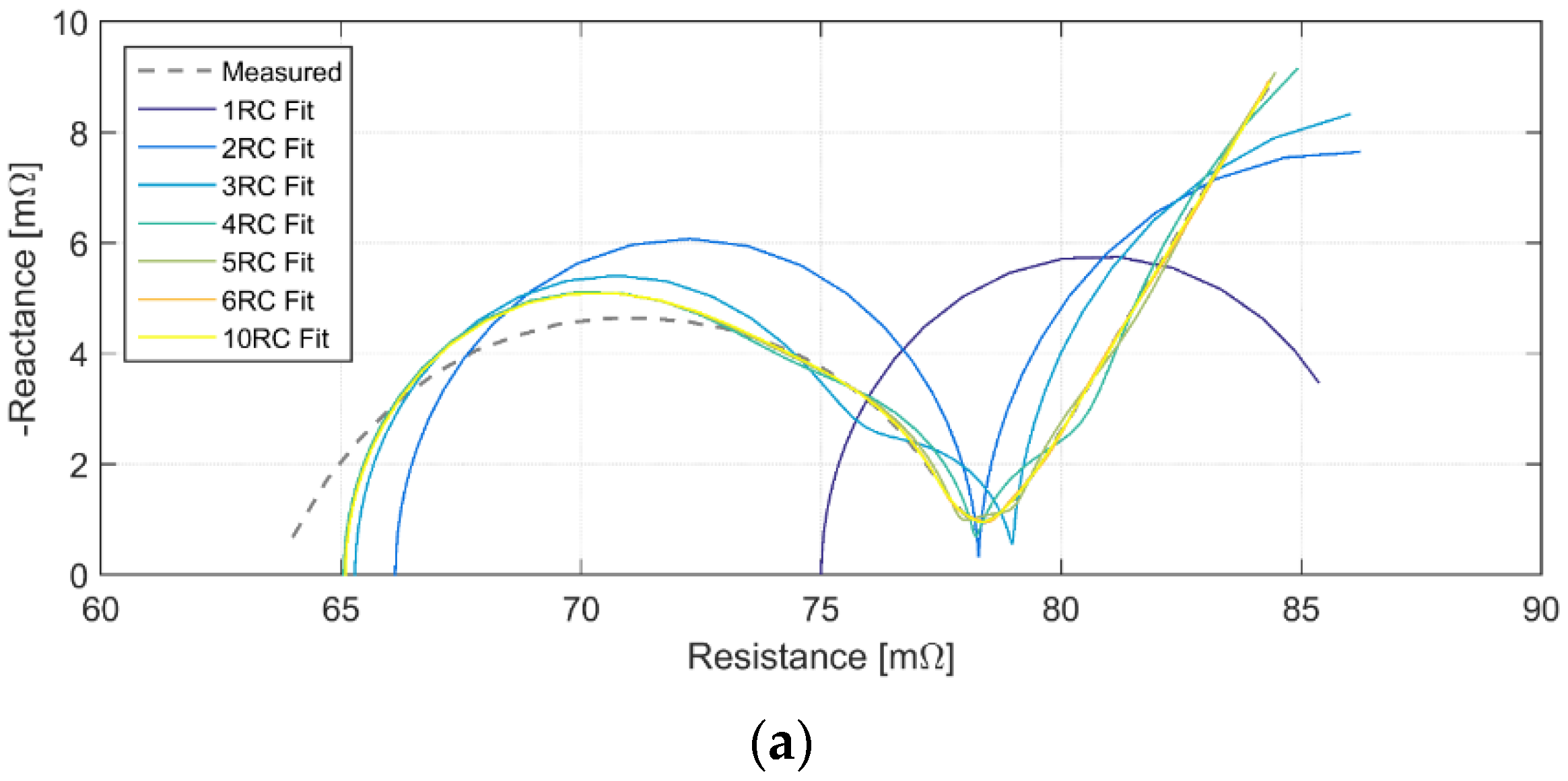
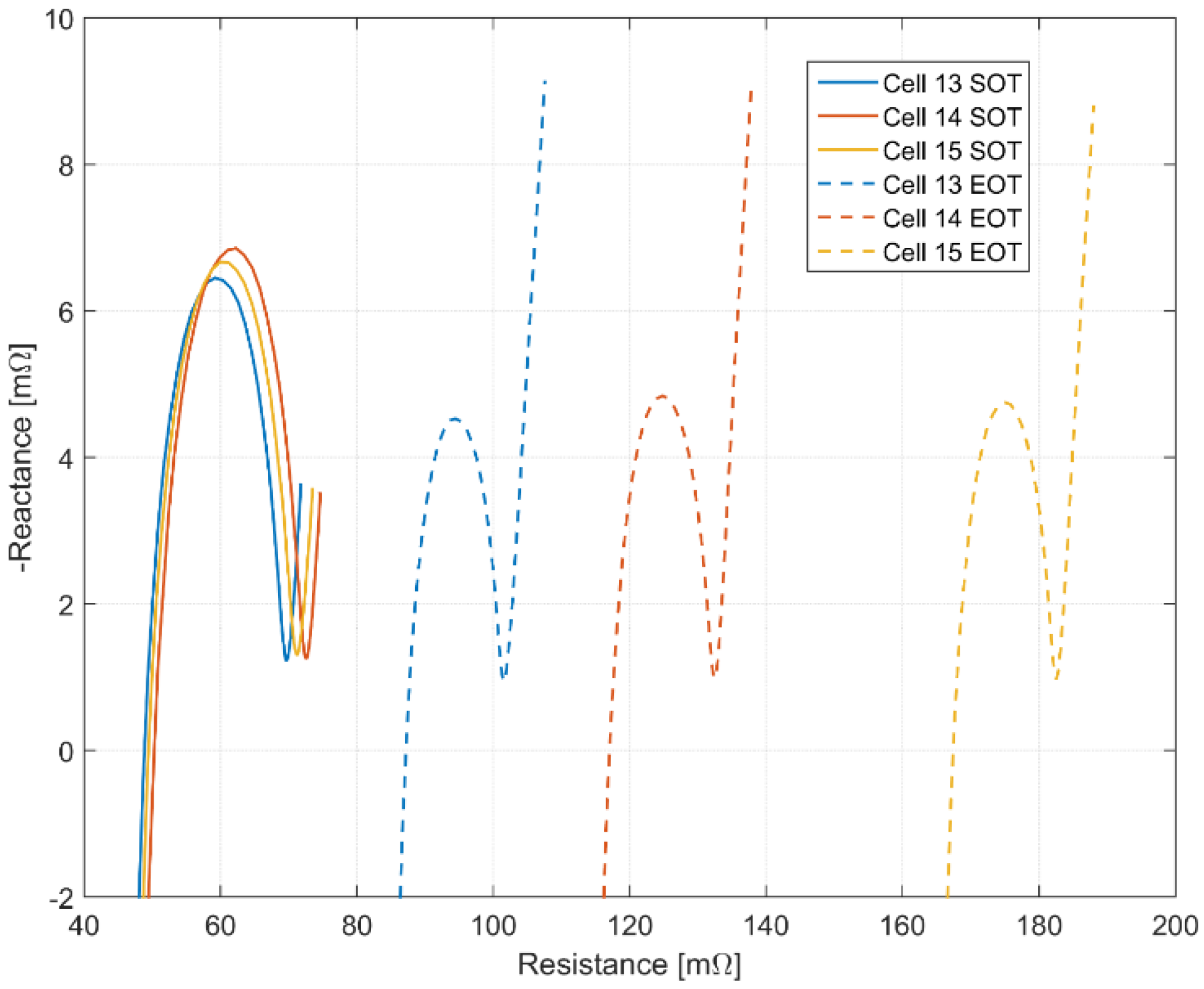
3.1. EIS Results for Post Vibration Aged Cells

Figure 4 shows the ohmic resistance (RO) of the cells at Start of Test (SOT) and End of Test (EOT) as measured by EIS. A complete explanation of EIS results is beyond the scope of this study and is already well documented in a number of academic and educational texts [27,28]. Figure 4 presents typical Nyquist plots of the cells pre and post vibration test for the cells condition to 50% SOC. Table 3 quantifies the increase in ohmic resistance obtained from the respective EIS data.
Typically, all samples displayed a significant increase ohmic resistance. Samples oriented in Z:Y axis and pre-conditioned to 50% SOC exhibited the highest increase out of the 50% SOC samples evaluated to SAE J2380. This is presented below in Table 3.

3.2. 1 C discharge capacity

Table 4. presents the 1C discharge capacity for each cell at SOT and EOT. From Table 4, it can be seen that the results show a tendency for samples orientated in the Z:Y axis and pre-conditioned to 50% SOC to exhibit a higher capacity fade than other 50% SOC samples.

4. Cell Modelling

Equivalent circuit models (ECMs) are commonly used to model cells due to their simplicity, ease of parameterization and real-time suitability compared to physics based models [29]. As well as being used to analyze cell and battery pack performance as part of a model-based design process [30], they can also be used for model-based state estimation of SOC and state of health (SOH) [3,31,32].
ECMs generally consist of a resistor connected in series with a number of resistor-capacitor (RC) pairs. A greater number of RC pairs increases the model bandwidth and accuracy, at the expense of computational complexity. Figure 5a shows a single cell ECM with NRC RC pairs. Several ECMs can be combined in parallel as in Figure 5b and/or in series as in Figure 5c. Compared to other types of cell, 18650 format cells have a low comparatively charge capacity. For larger applications, such as electric vehicles, the battery pack must contain many cells in parallel and series in order to meet power and energy requirements. For example, the Tesla Model S 85 kWh battery pack contains 7104 18650 format cells arranged into 96 series units, with each series unit containing 74 cells connected in parallel [33]. Understanding and managing the variations in the properties of each of these cells is important for optimizing the performance of the battery pack.
Dubarry et al. [34] showed that a series string of cells can be equated to a single cell model by accounting for the variations between cells. However, the authors note that this will become complex for larger numbers of cells, and the resulting model lacks the individual cell voltages which are important for assessing when the series string of cells has reach end of charge/ end of discharge. In [35] the authors find that string SOC estimation accuracy suffers when an averaged single cell model is used rather than individual cells. In [36], it is suggested that prior to assembling a series-parallel model of cells, the cells should be screened to ensure that only cells with very similar resistance and capacity are connected together. From this, it is assumed that cells in parallel can be equated to a single cell, as can cells in series. Combining both together, an arbitrary series-parallel module of cells can be represented by a single averaged ECM. However, As discussed in [37] there is no guarantee that the cells will remain similar over their life, and a single effective cell will not account for variations in current and SOC which can occur. Individual ECMs can also be used to implement model-based balancing strategies for cells in series [38].
The EIS data collected during the experimental phase were all obtained at 50% SOC. While it is known that cell impedance is a function of SOC, it is generally considered that there is little variation in the central SOC region at moderate temperatures [39,40] For the studies considered in this paper, the SOC of the cells is maintained between 30 and 70%. While the impedance remains constant, the open circuit voltage (OCV) is a nonlinear function of SOC. This can be incorporated into the cell model by using a lookup table.
In this case, OCV is implemented as a state and a parameter F is found using Equation (1), where Q is the 1C discharge capacity in Ah. This is then used to capture the relationship of OCV and current given by Equation (2). Each RC pair voltage is governed by Equation (3), and the terminal voltage of the cell given by Equation (4). Note that the DC resistance in the ECM is referred to as RD to avoid confusion with RO obtained from the EIS plots. Model errors and limits in bandwidth mean that the RD resistance may not equate exactly to the RO value for a given cell:
F ( O C V ) = 1 36 Q d O C V d S O C
O C V ˙ = F ( O C V ) i c e l l
v ˙ p = v p R p C p + i c e l l C p
v t = O C V + n = 1 N R C v p , n + R D i c e l l
These equations can be put into state-space form, which is well suited to modelling arbitrary time-domain signals such as the current applied under real-world driving conditions. For a single cell model with NRC pairs, the state equation are given by Equation (5), and the output equation by Equation (6).
[ O C V ˙ v ˙ p , 1 v ˙ p , 2 v ˙ p , N R C ] = [ 0 1 R p , 1 C p , 1 1 R p , 2 C p , 2 * 1 R p , N R C C p , N R C ] [ O C V v p , 1 v p , 2 v p , N R C ] + [ F ( O C V ) 1 C p , 1 1 C p , 2 1 C p , N R C ] i c e l l
v t = [ 1 1 1 ] [ O C V v p , 1 v p , 2 v p , N R C ] + R D i c e l l
The ECM impedance can be considered in the frequency domain, as a function of complex angular frequency s. The impedance for an ECM with NRC RC pairs is given in Equation (7):
Z ( s ) = R D + n = 1 N R C R p , n R p , n C p , n s + 1
An averaged parallel model (APM)—a single-cell effective model of the parallel-connected unit of cells— can also be created by combining each cell as per Equation (8). This averages out any variations in cell properties and as such cannot be used to explore the wider impact of combining cells in parallel. Similarly, an average series model (ASM) for cell impedance from a series string of N cells is given by Equation (9):
Z e f f = 1 k = 1 N 1 Z k
Z e f f = 1 N k = 1 N Z k
The output voltage can then be multiplied by N to obtain the string voltage. Using the method described and validated in [37], the individual ECMs can be combined into a parallel cell model, with the applied current as the input, and the terminal voltage as the output. Unlike the single effective cell model, this solution does not average out the variations in cell properties, and it means that the current through each cell can be calculated. In the paper, individual ECMs were parameterized from cells with different impedances resulting from charge-discharging cycling-induced ageing. A dynamic current load was applied to the cells while connected in parallel, and individual cell currents were also measured. The same applied load was used as an input to the parallel cell model so that cell currents and voltage could be calculated. The simulated cell currents were found to be accurate to 2% of the measured currents.
A summary of the parallel cell model is provided below, with the full derivation in [37]. The individual cells are combined into a single system by creating block diagonals of the state matrices in Equation (5) and selecting one set of output matrices from Equation (6) (since all of the cells are at the same voltage, only one output voltage is required and in this case the first cell is chosen to calculate voltage), which takes the form of Equation (10). The input matrix has to be updated at each time step by solving Equation (1). This system requires an input vector of cell currents, which is typically not available for a system of parallel cells. However, by applying Kirchoff’s laws, the cell currents can be calculated from knowledge of the cells’ states, model parameters and the known current applied to the parallel stack. This results in a linear system of equations which solves for a vector of cell currents based on each cell being at the same terminal voltage as its neighbor. These cell currents are given by Equation (11), which can be substituted into Equation (10) to give Equation (12):
[ x ˙ 1 x ˙ 2 x ˙ N ] = [ A 1 A 2   A N ] [ x 1 x 2 x N ] + [ B 1 B 2   B N ] [ i c e l l ,   1 i c e l l ,   2 i c e l l ,   N ] [ v t ] = [ C 1 0 0 0 ] [ x 1 x 2 x N ] + [ D 1 0 0 0 ] [ i c e l l ,   1 i c e l l ,   2 i c e l l ,   N ]
[ i c e l l   1 i c e l l   2 i c e l l   N ] = G R 1 ( E x + F i 1 )
G = [ 1 1 0 0 0 1 1 0 0 1 1 0 0 1 ] R = [ 1 0 0 0 0 ( R D , 1 + R D , 2 ) R D , 2 0 0 R D , 2 R D , N 1 0 0 R D , N 1 ( R D , N 1 + R D , N ) ] E = [ 0 0 0 1 1 1 1 0 0 0 1 1 1 1 0 0 0 0 1 1 1 1 ] F = [ 1 ( R D , 1 + 2 R c ) 0 0 ]
x ˙ = A x + B i 1 y = C x + D i 1 A = A + BGR 1 E B = BGR 1 F C = C + DGR 1 E D = DGR 1 F
This augmented solution demonstrates that the entire system of parallel states can be solved for while maintaining the same input (applied current) and output (cell voltage) and state-space structure as for a single cell model. This allows for the same simulation and analysis methods to be used as for single cells or cells in series.

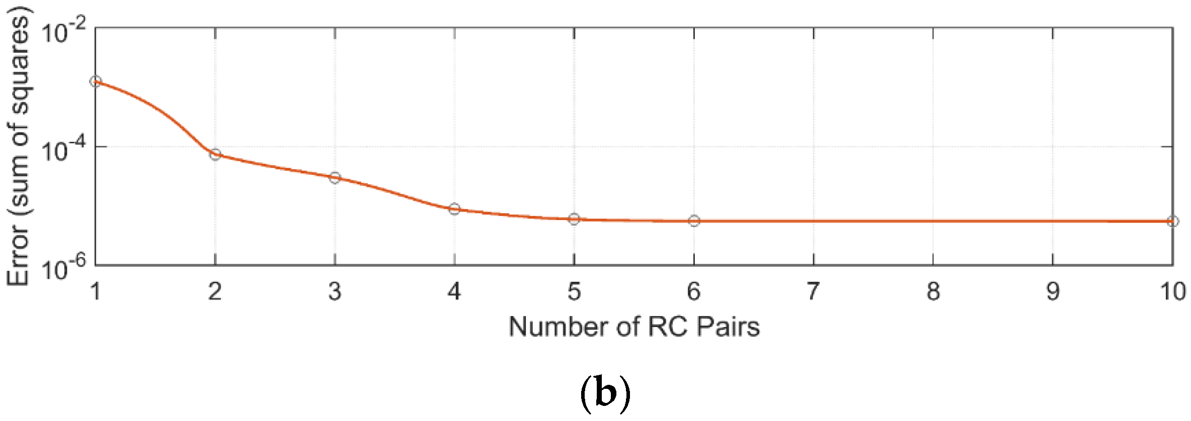
5. Model Parameterization

ECMs are not based on physical elements, and as such must be parameterized using system identification techniques rather than taking physical measurements of the cells. Each set of EIS data described in Section 3.1 was used to derive ECM parameters. To obtain the parameters, a nonlinear least squares optimization routine was used to apply the cost function in Equation (13). This adjusts the parameter vector θ in order to minimize the sum-of-squares difference between the experimentally measured impedance ZE, and the model impedance ZM, over Nf frequency points. The model impedance is calculated using Equation (7). The nonlinear least squares algorithm finds a local minimum to the cost function. There may be several local minima and depending on the starting point of the optimization, the global minimum may not be found. To reduce the sensitivity to initial conditions a multi-start algorithm was employed, which runs the local solver several times from different starting points, and then chooses the best solution from all of the runs:
arg min θ n = 1 N f ( Z n E Z n M ( θ ) ) 2
θ = [ R D , R p , 1 , C P , 1 , R p , 2 , , C P , N R C ]
The solution is also sensitive to the number of RC pairs chosen. The decision was made to cover the full frequency range of the EIS data up to the inductive region. For this type of cell, the crossing point of the impedance into the inductive region occurs at around 200 Hz. This is faster than a BMS will typically sample at [41] but previous research has found that there can be high frequency dynamics within parallel stacks [37] that the BMS may need to take account of in order to properly manage the individual cells.
An example of the Nyquist fits for cell 5 is shown in Figure 6a, and the associated errors in Figure 6b. It was found that a 4RC model provides an acceptable fit to the EIS data, with further RC pairs not significantly reducing the error. Several of the RC pairs are required to approximate a resistor-constant phase element pair which would better represent the curve shape, but cannot be easily translated to the time domain [42].
The model parameter results for the cells before and after ageing, are given in Table 5. As mentioned in Section 4, the limitations of the model mean that the RD values do not exactly match the RO values from Table 3, but the differences are all under 5 mΩ.

6. Simulation Case Studies

The ECM representations outlined in Section 4 have been implemented using the ode15 s solver in MATLAB (MathWorks, Natick, MA, USA), which was chosen because of its suitability to finding the solution to numerically stiff systems with a wide range of poles.

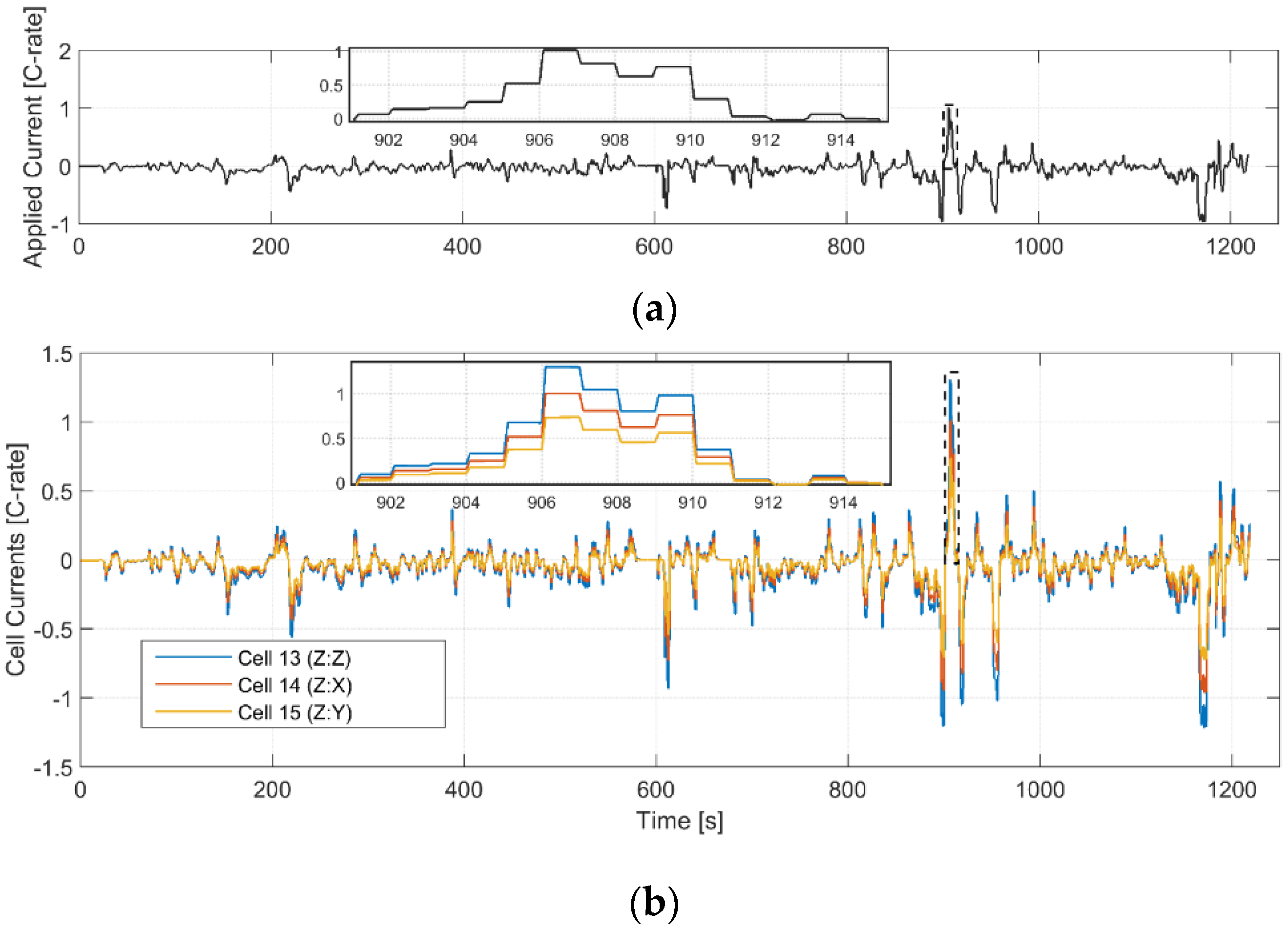
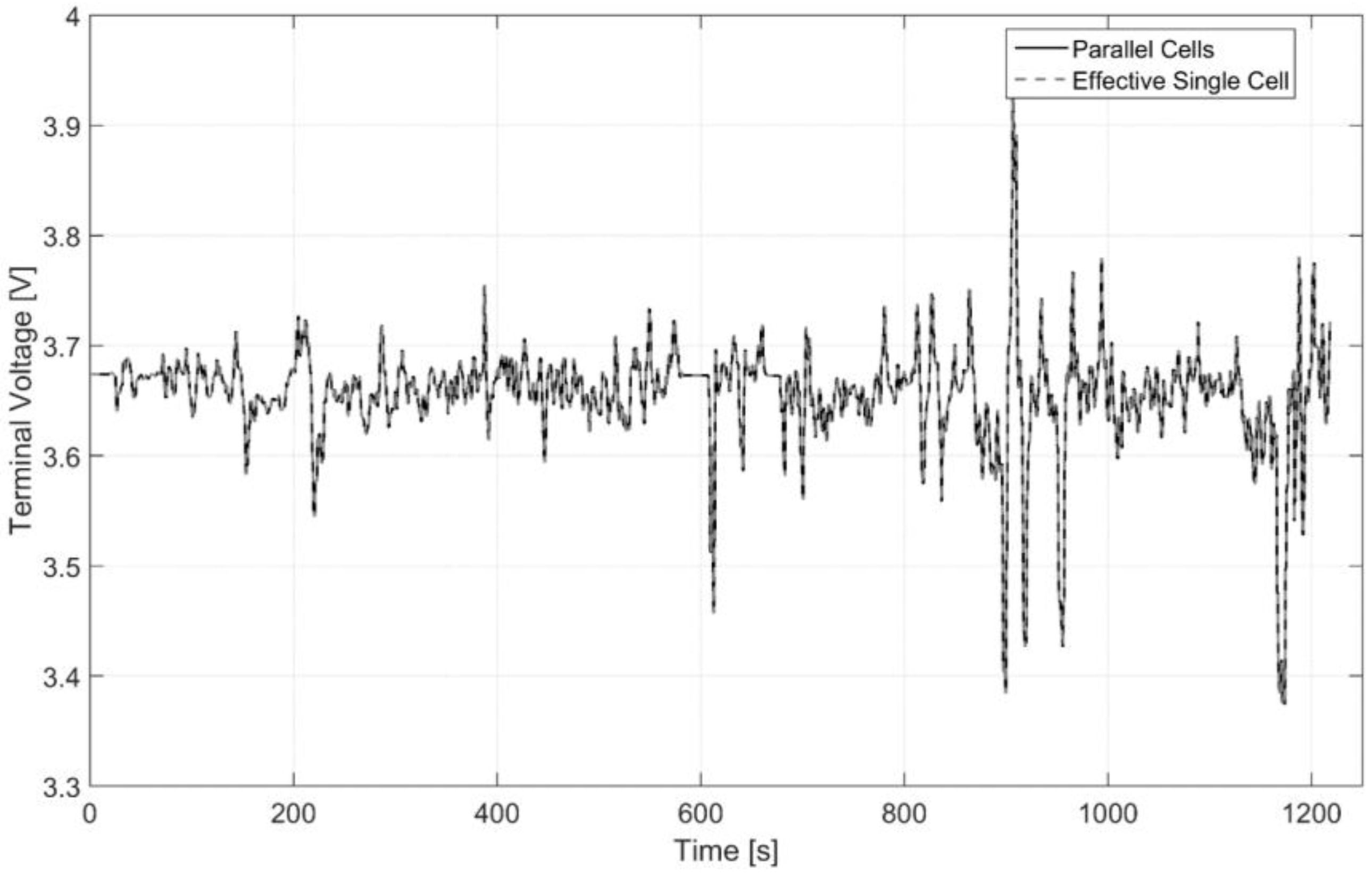
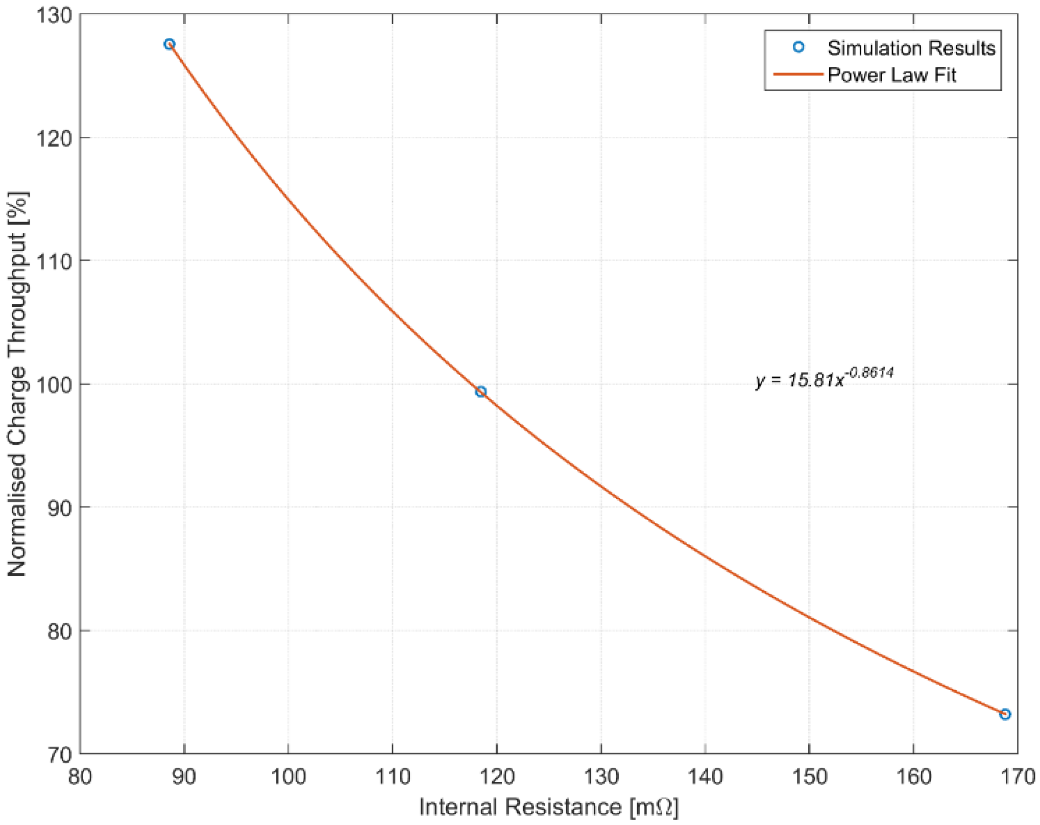
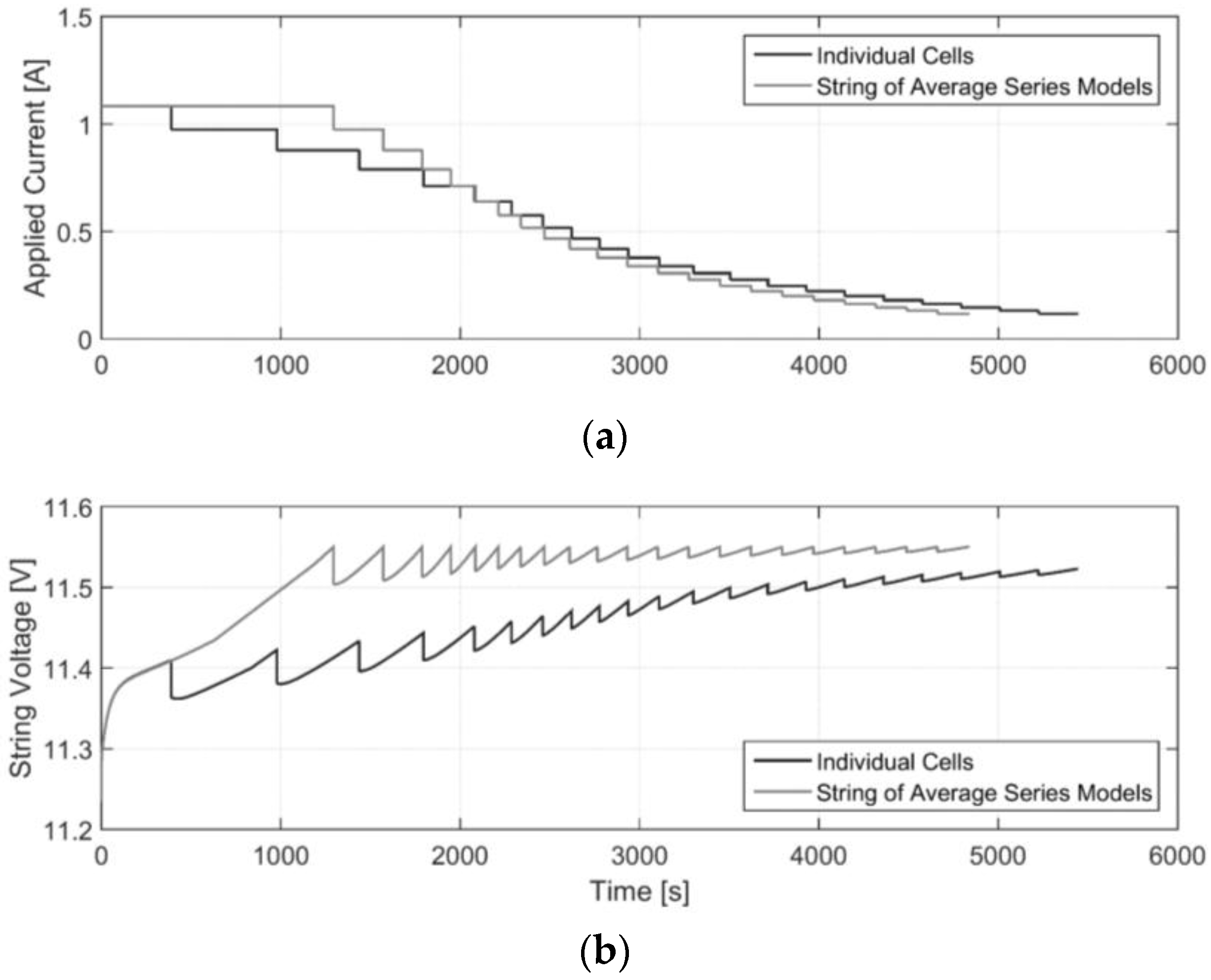
6.1. Parallel Cells Subjected to a HEV Profile

When cells with different impedances are connected in parallel, the individual cell currents can be significantly different. These currents are typically not monitored by a BMS and as such cannot be actively regulated during usage. To consider the impact that vibration may have on battery packs containing cells connected electrically in parallel, the ECMS for cells 13–15 are combined in parallel as in Figure 5b. This is compared with the APM defined by Equation (8).
A charge-sustaining drive cycle, typical of a HEV, is used for this simulation. Cells 13–15 are combined in parallel, and maintained at approximately 50% SOC. This drive cycle was derived from real-world driving data and is scaled such that the maximum current is 1C, and the cells started at 51% SOC, and ended at around 49% SOC. Figure 7a shows the applied current and individual cell currents (both as C-rates) for the aged cells, along with a zoomed-in Section. Figure 7b shows the corresponding cell currents. The terminal voltage simulation results in Figure 8 also show that even for aged cells, for a given current input, the calculated voltage out is almost identical to the parallel cell model, with a root mean squared (RMS) error of 0.15 mV.
In order to compare the relative loading of each cell, the nominal charge throughput is calculated. This is given for cell n by Equation (14), and can be considered an indication of the average current undergone by each cell, relative to the case of all cells being equal:
q t , n = 100 N p i c e l l , n 2 i a p p 2
The heat power and energy generated by the cell can be calculated using Equations (15) and (16) respectively. The heat energy per cell can be scaled relative to the heat energy calculated from the APM:
P h e a t = ( v t O C V ) i c e l l
E h e a t = P h e a t d t
The results, given in Table 6 show that the average loading of cell 13 is 27.5% higher than the nominal case, and cell 15 is 26.8% lower. This means that cell 13 undergoes 175% the loading of cell 15. The loading of the cells is relatively consistent over the course of the drive cycle. Current distribution within a parallel stack is driven by differences in OCV and impedance. The small SOC change means that the OCV of each cell remains similar, with less than 5 mV difference between cells. Therefore the difference in impedance (resulting from cell vibration) is what is causing cell currents to differ in this case. Previous work has shown that this can cause significant dynamic variation in cell currents [37]. However, that study used cells aged by different mechanism. Those cells had a very similar DC resistance, but differences in solid-electrolyte interphase (SEI) build up resulted in a notably different charge transfer resistance. This meant that the impedance variation between the cells was a function of frequency. However, for these cells aged primarily through vibration, the DC resistance has shifted significantly, with little SEI build-up. This means that there is always a large difference in impedance between cells regardless of the frequency, and the difference in cell currents is primarily driven by the ohmic resistance of the model. This, along with the similar OCVs of each cell, means that the proportion of heat energy generated by each cell is very similar to the proportion of current loading.
In Figure 9, the nominal charge throughput is plotted as a function of ohmic resistance. A power-law trend line has also been calculated using a least squares approach. A power law was chosen because, unlike a polynomial or exponential fit, it behaves logically when extrapolating: as resistance tends to infinity, the charge throughput tends to zero, and as resistance tends to zero, charge throughput tends to infinity.
Since these currents are typically not measured by a BMS, it is important to design the pack such that these variations are accounted for and individual cells are not taken outside of their intended operating window during the entirety of the battery pack’s life. The differences in current may cause the cells to age by different amounts, which could be unpredictable and must be carefully analyzed and managed. The thermal management system of the battery pack must also be designed, from a hardware and BMS perspective, to be able to reduce any temperature differences which may arise because of impedance variation. Impedance generally decreases with temperature [39], which could further increase the variation in cell currents if not properly managed.

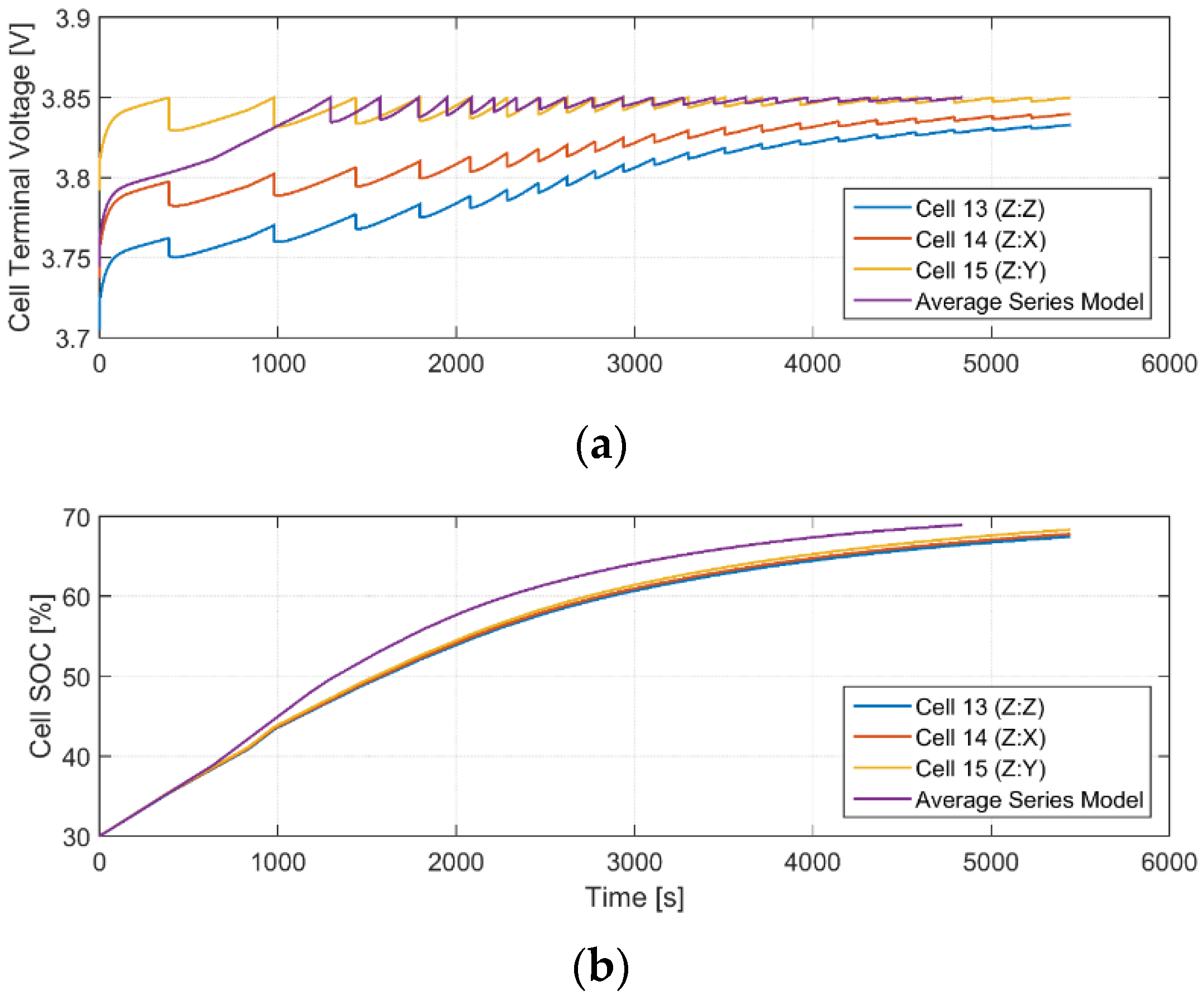
6.2. Charging Cells in Series

When cells are connected in series, the cell current is the same for each cell, but each cell can be at a different voltage. Differences in voltage can occur due to cells being at unequal SOCs and impedance variation between cells. Variations can occur for a variety of reasons, including differences in capacity, self-discharge rate and temperature [43,44].
Constant current-constant voltage charging is commonly used to charge cells. However, this cannot be directly applied with a module of cells in series. The charging strategy considered here is to charge at a constant current (C/2 charging rate) until any one cell reaches the maximum cell voltage. The applied current is then reduced by 10%, and constant current charging continues until one cell again reaches maximum voltage. The current is reduced by another 10%, and this process is repeated until the charging current is below a certain threshold. For this study, ECMs for cells 13–15 are connected in series as in Figure 5c, and this is compared against three ASMs in series. The ASM is found by applying Equation (9) to the measured impedance of cells 13–15, and then identifying the parameters as described in Section 5.
As can be seen in Figure 10a, there is almost a 90 mV difference between cells 14 and 15, despite there being very little difference in SOC. This means that the higher impedance cell reaches its maximum voltage before the other, and so the lower impedance cell is not charged as much as it could be. Figure 10b shows that the ASM SOC is 1.5% higher than the lowest SOC of the string of individual ECMs despite all cells starting from the same SOC. For a series string of cells, the lowest cell SOC is a strong indicator of the overall pack performance [3]. This difference would increase if charging occurred over a wider SOC window or at a higher current.
Cell balancing systems are used to remove variations in energy between cells in series [45,46]. Cell voltage is commonly used as a metric of imbalance because it is a direct measurement rather than an estimate, as is the case for SOC or charge level. In this case the SOCs remain similar throughout charging, so there is no significant SOC imbalance. However, there is a significant voltage imbalance due to the applied load and differences in impedance. As such if balancing was performed over the charging period and activated based on the voltage difference, the result would be that once the pack had finished charging and the applied load was zero, the SOCs and terminal voltages of the cells would actually be imbalanced.
In Figure 11, the three cell string is compared with the same charging simulation for three of the ASMs in series. Figure 11a shows that charging current is generally higher for the ASM string, and as such reaches end of charge 549 s quicker. Figure 11b shows that the string voltage is also higher for the ASM case, increasing the available power of the string.

7. Further Work

One of the limitations of the methodology employed within this study is that electrical characterization data was only measured at SOT and EOT from the vibration aged cells. As a result, no discussion or conclusions can be made about the rate of degradation throughout the vehicle’s life and therefore the gradual change on cell impedance on the robustness of the BMS algorithms for managing change imbalance within the complete battery pack. It is recommended that a future study should characterize the cells at intermediate points during the test program, e.g. intervals representative of 10,000 miles of vehicle use. This would facilitate further investigation into both the absolute value of degradation, but also the expected in-service rate of capacity and power fade over the life of the vehicle. The variance in impedance between the aged cells means that a balancing system is necessary to manage the available capacity over the life of a battery pack. Model-based design using these ECMs could be used to design a balancing control system to maximize the available battery pack energy and account for the variations in impedance and capacity. Other BMS functionality, such as detecting a cell end of life condition or failure through vibration can also be explored using model-based techniques. Vibration causes a notable shift in ohmic resistance, which is distinct from other major types of ageing [39], and it may be possible for a BMS to classify the type of ageing based on this information.

8. Conclusions

Using experimental data and previously validated mathematical cell models, it has been shown that the ageing caused by vibration can have a significant impact on various BMS functions and the battery pack itself. For cells connected in parallel, the thermal management system must be designed to be reduce variations in temperature which can occur through different current loading between cells. Significant differences in cell current are also shown to occur owing to the impedance differences between cells aged through vibration. Since the individual cell currents are not measured, it is important that the battery pack is designed so that each cell is not taken outside its intended operating window. When aged cells are connected in series, variations in impedance limit the ability to fully charge the series string, reducing the available power and increasing the charging time for the complete battery system.

Acknowledgments

The research presented within this paper is supported by the Engineering and Physical Science Research Council (EPSRC-EP/I01585X/1) through the Engineering Doctoral Centre in High Value, Low Environmental Impact Manufacturing. The research was undertaken in collaboration with the WMG Centre High Value Manufacturing Catapult (funded by Innovate UK) and Jaguar Land Rover. The authors would also like to express their gratitude to Millbrook Proving Ground Ltd (Component Test Laboratory) for their support and advice throughout the durability test program.

Author Contributions

Thomas Bruen—Primary researcher and lead author. James Michael Hooper—Experimental researcher (durability characterization) and co-author. James Marco—Academic research supervision and co-author. Miguel Gama—Industrial research support and peer-review. Gael Henri Chouchelamane—Experimental researcher (electrical characterization) and co-author.

Conflicts of Interest

The authors declare no conflict of interest.

References

  1. Jackson, N. Technology Road Map, R+D Agenda and UK Capabilities. In Proceedings of the Cenex Low Carbon VehicleEvent, Millbrook Proving Ground, Bedfordshire, UK, 15–16 September 2010; pp. 1–16.
  2. Parry-Jones, R.; Cable, V. Driving Success—A Strategy for Growth and Sustainability in the UK Automotive Sector; Automotive Council UK: London, UK, 2013. [Google Scholar]
  3. Lu, L.; Han, X.; Li, J.; Hua, J.; Ouyang, M. A review on the key issues for lithium-ion battery management in electric vehicles. J. Power Sources 2013, 226, 272–288. [Google Scholar] [CrossRef]
  4. Xing, Y.; Ma, E.W.M.; Tsui, K.L.; Pecht, M. Battery Management Systems in Electric and Hybrid Vehicles. Energies 2011, 4, 1840–1857. [Google Scholar] [CrossRef]
  5. Day, J. Johnson Controls’ Lithium-Ion Batteries Power Jaguar Land Rover’s 2014 Hybrid Range Rover. Available online: http://johndayautomotivelectronics.com/johnson-controls-lithium-ion-batteries-power-2014-hybrid-range-rover/ (accessed on 28 November 2015).
  6. Rawlinson, P.D. Integration System for a Vehicle Battery Pack. US8833499 B2, 16 September 2014. [Google Scholar]
  7. Berdichevsky, G.; Kelty, K.; Straubel, J.B.; Toomre, E.; Motors, T. The Tesla Roadster Battery System, 2nd ed.; Tesla Motors: Palo Alto, CA, USA, 2007. [Google Scholar]
  8. Kelty, K. The battery technology behind the wheel. Available online: http://asia.stanford.edu/us-atmc/wordpress/wp-content/uploads/2010/12/ee402s-04022009-tesla.pdf (accessed on 23 March 2016).
  9. Paterson, A. Our Guide to Batteries. Available online: http://www.jmbatterysystems.com/JMBS/media/JMBS/Technology/Axeon-Guide-to-Batteries-2nd-edition.pdf (accessed on 23 March 2016).
  10. Anderman, M. Tesla Motors: Battery Technology, Analysis of the Gigafactory, and the Automakers’ Perspectives; Advanced Automotive Batteries: 9204 Citron Way, Oregon House, CA, USA, 2014; pp. 1–39. [Google Scholar]
  11. Karbassian, A.; Bonathan, D.P. Accelerated Vibration Durability Testing of a Pickup Truck Rear Bed (2009-01-1406). SAE Int. 2009, 1–5. [Google Scholar] [CrossRef]
  12. Risam, G.S.; Balakrishnan, S.; Patil, M.G.; Kharul, R.; Antonio, S. Methodology for Accelerated Vibration Durability Test on Electrodynamic Shaker. SAE Int. 2006, 1, 1–9. [Google Scholar]
  13. Harrison, T. An Introduction to Vibration Testing; Bruel and Kjaer Sound and Vibration Measurement: Naerum, Denmark, 2014. [Google Scholar]
  14. Hooper, J.M.; Marco, J. Experimental Modal Analysis of Lithium-Ion Pouch Cells. J. Power Sources 2015, 285, 247–259. [Google Scholar] [CrossRef]
  15. Moon, S.-I.; Cho, I.-J.; Yoon, D. Fatigue life evaluation of mechanical components using vibration fatigue analysis technique. J. Mech. Sci. Technol. 2011, 25, 611–637. [Google Scholar] [CrossRef]
  16. Halfpenny, A.; Hayes, P. Fatigue Analysis of Seam Welded Structures using nCode DesignLife. In Proceedings of 2010 European HyperWorks Technology Conference, Versailles, France, 27–29 October 2010; pp. 1–21.
  17. Halfpenny, A. Methods for Accelerating Dynamic Durability Tests. In Proceedings of the 9th International Conference on Recent Advances in Structural Dynamics, Southampton, UK, 17–19 July 2006; pp. 1–19.
  18. Brand, M.J.; Schuster, S.F.; Bach, T.; Fleder, E.; Stelz, M.; Glaser, S.; Muller, J.; Sextl, G.; Jossen, A.A.; Gläser, S.; et al. Effects of vibrations and shocks on lithium-ion cells. J. Power Sources 2015, 288, 62–69. [Google Scholar] [CrossRef]
  19. Hooper, J.; Marco, J.; Chouchelamane, G.; Lyness, C. Vibration Durability Testing of Nickel Manganese Cobalt Oxide (NMC) Lithium-Ion 18650 Battery Cells. Energies 2016, 9, 27. [Google Scholar] [CrossRef]
  20. Vibration Testing of Electric Vehicle Batteries; Society of Automotive Engineers (SAE): Warrendale, PA, USA, 2013; pp. 1–7.
  21. Hooper, J. Study into the Vibration Inputs of Electric Vehicle Batteries. Master’s Thesis, Cranfield University, Cranfield, Bedfordshire, UK, December 2012. [Google Scholar]
  22. Hooper, J.M.; Marco, J. Characterising the in-vehicle vibration inputs to the high voltage battery of an electric vehicle. J. Power Sources 2014, 245, 510–519. [Google Scholar] [CrossRef]
  23. Barai, A.; Chouchelamane, G.H.; Guo, Y.; McGordon, A.; Jennings, P. A study on the impact of lithium-ion cell relaxation on electrochemical impedance spectroscopy. J. Power Sources 2015, 280, 74–80. [Google Scholar] [CrossRef]
  24. Hooper, J.; Marco, J. Understanding Vibration Frequencies Experienced by Electric Vehicle Batteries. In Proceedings of the 4th Hybrid and Electric Vehicles Conference (HEVC), London, UK, 6–7 Novermber 2013; pp. 1–6.
  25. Harrison, T. Random Vibration Theory; Bruel and Kjaer Sound and Vibration Measurement: Naerum Denmark, 2014. [Google Scholar]
  26. Harrison, T. The Vibration System; Bruel and Kjaer Sound and Vibration Measurement: Naerum, Denmark, 2014. [Google Scholar]
  27. Chouchelamane, G. Electrochemical Impedance Spectroscopy; Warwick Manufacturing Group: Warwick, UK, 2013. [Google Scholar]
  28. Birkl, C.R.; Howey, D.A. Model Identification and Parameter Estimation for LiFePO4 Batteries. In Proceedings of the 4th Hybrid and Electric Vehicles Conference (HEVC), London, UK, 6–7 Novermber 2013; pp. 1–6.
  29. Hu, X.; Li, S.; Peng, H. A comparative study of equivalent circuit models for Li-ion batteries. J. Power Sources 2012, 198, 359–367. [Google Scholar] [CrossRef]
  30. He, H.; Xiong, R.; Fan, J. Evaluation of Lithium-Ion Battery Equivalent Circuit Models for State of Charge Estimation by an Experimental Approach. Energies 2011, 4, 582–598. [Google Scholar] [CrossRef]
  31. Seaman, A.; Dao, T.-S.; McPhee, J. A survey of mathematics-based equivalent-circuit and electrochemical battery models for hybrid and electric vehicle simulation. J. Power Sources 2014, 256, 410–423. [Google Scholar] [CrossRef]
  32. Fleischer, C.; Waag, W.; Heyn, H.-M.; Sauer, D.U. On-line adaptive battery impedance parameter and state estimation considering physical principles in reduced order equivalent circuit battery models. Part 1. Requirements, critical review of methods and modeling. J. Power Sources 2014, 260, 276–291. [Google Scholar] [CrossRef]
  33. The Tesla Battery Report. Available online: http://advancedautobat.com/industry-reports/2014-Tesla-report/Extract-from-the-Tesla-battery-report.pdf (accessed on 22 October 2014).
  34. Dubarry, M.; Vuillaume, N.; Liaw, B.Y. From single cell model to battery pack simulation for Li-ion batteries. J. Power Sources 2009, 186, 500–507. [Google Scholar] [CrossRef]
  35. Truchot, C.; Dubarry, M.; Liaw, B.Y. State-of-charge estimation and uncertainty for lithium-ion battery strings. Appl. Energy 2014, 119, 218–227. [Google Scholar] [CrossRef]
  36. Kim, J.; Cho, B.H. Screening process-based modeling of the multi-cell battery string in series and parallel connections for high accuracy state-of-charge estimation. Energy 2013, 57, 581–599. [Google Scholar]
  37. Bruen, T.; Marco, J. Modelling and experimental evaluation of parallel connected lithium ion cells for an electric vehicle battery system. J. Power Sources 2016, 310, 91–101. [Google Scholar] [CrossRef]
  38. Bruen, T.; Marco, J.; Gama, M. Model Based Design of Balancing Systems for Electric Vehicle Battery Packs. IFAC-PapersOnLine 2015, 48, 395–402. [Google Scholar] [CrossRef]
  39. Waag, W.; Käbitz, S.; Sauer, D.U. Experimental investigation of the lithium-ion battery impedance characteristic at various conditions and aging states and its influence on the application. Appl. Energy 2013, 102, 885–897. [Google Scholar] [CrossRef]
  40. Andre, D.; Meiler, M.; Steiner, K.; Wimmer, C.; Soczka-Guth, T.; Sauer, D.U. Characterization of high-power lithium-ion batteries by electrochemical impedance spectroscopy. I. Experimental investigation. J. Power Sources 2011, 196, 5334–5341. [Google Scholar] [CrossRef]
  41. Mueller, K.; Tittel, D.; Graube, L.; Sun, Z.; Luo, F. Optimizing BMS Operating Strategy Based on Precise SOH Determination of Lithium Ion Battery Cells. In Proceedings of the International Federation of Automotive Engineering Societies 2012 World Automotive Congress, Beijing, China, 27–30 November 2012; pp. 807–819.
  42. Waag, W.; Käbitz, S.; Sauer, D.U. Application-specific parameterization of reduced order equivalent circuit battery models for improved accuracy at dynamic load. Measurement 2013, 46, 4085–4093. [Google Scholar] [CrossRef]
  43. Xu, J.; Li, S.; Mi, C.; Chen, Z.; Cao, B. SOC Based Battery Cell Balancing with a Novel Topology and Reduced Component Count. Energies 2013, 6, 2726–2740. [Google Scholar] [CrossRef]
  44. Zhang, Z.; Sisk, B. Model-Based Analysis of Cell Balancing of Lithium-ion Batteries for Electric Vehicles. SAE Int. J. Alt. Power 2013, 2, 379–388. [Google Scholar] [CrossRef]
  45. Moore, S.W.; Schneider, P.J. A Review of Cell Equalization Methods for Lithium Ion and Lithium Polymer Battery Systems. SAE Publ. 2001, 2001010959, 1–7. [Google Scholar]
  46. Gallardo-Lozano, J.; Romero-Cadaval, E.; Milanes-Montero, M.I.; Guerrero-Martinez, M.A. Battery equalization active methods. J. Power Sources 2014, 246, 934–949. [Google Scholar] [CrossRef]
Figure 1. Schematic of test process.
Energies 09 00255 g001
Figure 2. Society of Automotive Engineers (SAE) J2380 vibration power spectral density (PSD) profiles for testing samples 13 to 15 [20].
Energies 09 00255 g002
Figure 3. (a) Axis convention of vehicle vibration durability profiles; (b) Axis convention of cells.
Energies 09 00255 g003
Figure 4. Electrochemical impedance spectroscopy (EIS) start of test (SOT) and end of test (EOT) results.
Energies 09 00255 g004
Figure 5. (a) A single cell equivalent circuit model (ECM) with NRC pairs; (b) Three cells in parallel with a current source; (c) Three cells in series with a current source.
Energies 09 00255 g005
Figure 6. (a) Comparison of impedance accuracy of cell 5 for various model orders; (b) Sum of squares error between model and measured impedance for various model orders.
Energies 09 00255 g006aEnergies 09 00255 g006b
Figure 7. (a) Current applied to the parallel unit of cells; (b) Individual cell currents.
Energies 09 00255 g007
Figure 8. Terminal voltage over the drive cycle for the parallel cell model and effective single cell model.
Energies 09 00255 g008
Figure 9. Normalized charge throughput as a function of RO resistance.
Energies 09 00255 g009
Figure 10. (a) Terminal voltage for the three individual cells and average series cell; (b) SOC for the three individual cells and average series cell.
Energies 09 00255 g010
Figure 11. (a) Charging current for a string of individual cells, and a string of mean series model cells; (b) Total voltage for a string of individual cells, and a string of mean series model cells.
Energies 09 00255 g011
Table 1. Test sample information.
Sample No in [1] *Test ProfileSOC (%)Cell Orientation (Vehicle Axis: Cell Axis)
4Control sample—In permanent storage50%Control
5Control sample—Followed J2380 test samples50%Control
13J238050%Z:Z
14J238050%Z:X
15J238050%Z:Y
* Samples 1 to 3, 6 to 12 and 16 to 18 are omitted as they were not evaluated in accordance with SAE J2380 or not conditioned to 50% SOC in [1].
Table 2. Society of Automotive Engineers (SAE) J2380 vibration profiles schedule.
Profile Description and GRMS LevelDuration (HH:MM)Test Cumulative Duration (HH:MM)
Z Axis Schedule
Subject cells to 9 min of Z-axis profile 1 at 1.9 Grms in the Z axis orientation of the cells under assessment.00:0900:09
Subject cells to 5 h and 15 min of Z-axis profile 1 at 0.75 Grms in the Z axis orientation of the cells under assessment.05:1505:24
Subject cells to 9 min of Z-axis profile 2 at 1.9 Grms in the Z axis orientation of the cells under assessment.00:0905:33
Subject cells to 5 h and 15 min of Z-axis profile 2 at 0.75 Grms in the Z axis orientation of the cells under assessment.05:1510:48
Subject cells to 9 min of Z-axis profile 3 at 1.9 Grms in the Z axis orientation of the cells under assessment.00:0910:57
Subject cells to 5 h and 15 min of Z-axis profile 3 at 0.75 Grms in the Z axis orientation of the cells under assessment.05:1516:12
X Axis Schedule
Subject cells to 5 min of X & Y-axis profile at 1.5 Grms in the X axis orientation of the cells under assessment.00:0516:17
Subject cells to 19 h of X & Y-axis profile at 0.4 Grms in the X axis orientation of the cells under assessment.19:0035:17
Subject cells to 5 min of X & Y-axis profile at 1.5 Grms in the X axis orientation of the cells under assessment.00:0535:22
Subject cells to 19 h of X & Y-axis profile at 0.4 Grms in the X axis orientation of the cells under assessment.19:0054:22
Y Axis Schedule
Subject cells to 5 min of X & Y-axis profile at 1.5 Grms in the Y axis orientation of the cells under assessment.00:0554:27
Subject cells to 19 h of X & Y-axis profile at 0.4 Grms in the Y axis orientation of the cells under assessment.19:0073:27
Subject cells to 5 min of X & Y-axis profile at 1.5 Grms in the Y axis orientation of the cells under assessment.00:0573:32
Subject cells to 19 h of X & Y-axis profile at 0.4 Grms in the Y axis orientation of the cells under assessment.19:0092:32
Total-92:32
Table 3. Electrochemical impedance spectroscopy (EIS) ohmic resistance (RO) results for all tested samples.
Sample NoSOCOrientationSOT (mΩ)EOT (mΩ)Percentage Change (%)
1550 %Z:Y46.4164.5254.53
1450 %Z:X47.3114.2141.44
1350 %Z:Z46.084.082.61
550 %Control49.660.822.58
SOTEOT
Standard deviation for tested 50% SOC samples (mΩ)0.6740.67
Mean for tested 50% SOC samples (mΩ)46.57120.90
Table 4. Summary of change in 1C discharge capacity performance of all test cells.
Sample No.SOC (%)OrientationCell Capacity at SOT (Ah)Cell Capacity at EOT (Ah)Percentage Change in Ah (%)
1550%Z:Y2.182.14−1.83
1350%Z:Z2.232.19−1.79
1450%Z:X2.152.170.93
550%Control 2.182.190.46
SOTEOT
Standard deviation for tested 50% SOC samples (Ah)0.0400.025
Mean for tested 50% SOC samples (Ah)2.192.17
Table 5. Parameterization results for cells 5, 13, 14 and 15.
Cell AgeSOTEOT
Cell Number51314155131415
RD0.054160.050340.051830.050970.065060.088580.118460.16881
Rp10.010840.010670.010860.010740.009150.009210.009330.00927
Cp10.384180.396930.381670.393260.119620.132510.117530.1235
Rp20.008470.007740.00870.008340.004010.003690.004490.00426
Cp23.06743.46272.98013.18162.10072.67891.84832.0417
Rp30.001740.001710.001770.00180.002530.002680.002430.00246
Cp3355.19465.36331.11339.43481.78508.56570.11540.8
Rp40.008690.010020.008810.008260.023310.025620.027540.02574
Cp43150.53191.93155.63041.61459.91454.314981513.7
Table 6. Summary of key results from parallel cell simulation.
Cell Sample Number131415
Relative current loading (%)New101.998.299.9
Aged127.599.473.2
Relative heat energy (%)New101.998.299.9
Aged126.899.573.8

