Quantifying the Impact of Feedstock Quality on the Design of Bioenergy Supply Chain Networks

Abstract

Logging residues, which refer to the unused portions of trees cut during logging, are important sources of biomass for the emerging biofuel industry and are critical feedstocks for the first-type biofuel facilities (e.g., corn-ethanol facilities). Logging residues are under-utilized sources of biomass for energetic purposes. To support the scaling-up of the bioenergy industry, it is essential to design cost-effective biofuel supply chains that not only minimize costs, but also consider the biomass quality characteristics. The biomass quality is heavily dependent upon the moisture and the ash contents. Ignoring the biomass quality characteristics and its intrinsic costs may yield substantial economic losses that will only be discovered after operations at a biorefinery have begun. This paper proposes a novel bioenergy supply chain network design model that minimizes operational costs and includes the biomass quality-related costs. The proposed model is unique in the sense that it supports decisions where quality is not unrealistically assumed to be perfect. The effectiveness of the proposed methodology is proven by assessing a case study in the state of Tennessee, USA. The results demonstrate that the ash and moisture contents of logging residues affect the performance of the supply chain (in monetary terms). Higher-than-target moisture and ash contents incur in additional quality-related costs. The quality-related costs in the optimal solution (with final ash content of 1% and final moisture of 50%) account for 27% of overall supply chain cost. Based on the numeral experimentation, the total supply chain cost increased 7%, on average, for each additional percent in the final ash content.

1. Introduction

Bioenergy has been regarded as an important alternative energy source that has the potential to help nations alleviate their reliance on petroleum energy, thereby, producing positive impacts on the economy, the environment, and the society [1]. Diverse studies have concluded that the production of bioenergy is expected to increase in the years to come [2,3,4]. One of the most important obstacles for the bioenergy utilization is related to the high feedstock-logistics costs and the dearth of technologies to convert biomass into useful forms of energy [5]. “Feedstock logistics” include the necessary operations to harvest the biomass and transport it from the reference site to the pertinent biorefinery. These operations must ensure that the delivered feedstocks meet a set of physical and chemical quality specifications [1]. To date, most assessments of the biofuel feedstocks availability have focused on quantifying the feasibility of having enough biomass supply to meet the biofuel production goals at minimal cost. However, as the industry grows and matures, concerns related to the quality variability of the feedstock arise and have become critical in the energy conversion process and in the market environment. The inherent variability of the biomass quality is a barrier that restrains the development of reliable bioenergy energy conversion processes. Hence, advanced biomass supply systems and practices are needed to reduce the variability of the biomass quality parameters, such as the ash and the moisture contents [6].

One of the main challenges of the bioenergy industry consists in quantifying the impacts of the biomass quality across the supply chain (SC). Despite bioenergy being an emerging industry, it inherited concepts and models from the well-established agricultural and logging industries. The primary objective in the traditional biomass feedstock logistics modeling approaches consists in reducing the overall cost of the SC, under the assumption that the biomass quality specifications are consistent and similar to forage and pulpwood [6]. The single objective of minimizing the total cost (e.g., composed of the feedstock base cost and the logistics and processing operations costs, among others) may produce considerable negative impacts on the biomass quality and, thereby, on the performance of bioenergy SCs. In practice, bioenergy SCs often work with highly variable and/or poor quality biomass characteristics, which in turn impacts the bioenergy conversion process. A recent paper from Idaho National Laboratory [6] raises the concern that research on feedstock quality still lacks proper theoretical support and that conventional approaches often disregard quality-related issues by focusing solely on decreasing the logistics cost. The emphasis of cost over quality is exemplified by the current pricing structure of the biomass, which is based on the measure “dollar per dry ton” instead of “dollar per clean dry carbohydrate.”

Practitioners who have reached pilot-scale operations, which require large quantities of feedstock, have experienced considerable differences between “pristine” and “field-run” biomass [7]. The scaling-up process is often accompanied by an undesirable level of risk, which becomes a very important parameter to consider in the bioenergy industry as new technologies with associated quality specifications evolve from the laboratory to the commercial settings [8]. For example, consider the scenario in which the biorefinery equipment, designed to work with a biomass moisture content of approximately 10%, has to work with a moisture content of 30% continuously throughout an entire year. For this particular case, the biorefinery would incur larger operation and maintenance costs. Equivalently, consider the financial losses if one load of feedstock yields 90 gallons/ton and another load yields 60 gallons/ton. Kenney et al. [6] demonstrated through the analysis of the biomass quality characteristics that these scenarios are very likely to occur in practice. The biomass quality is critically dependent upon the moisture, ash and sugar contents, as well as the particle morphology of the feedstock, among other variables. Ignoring the biomass quality variations and, thus, the associated costs when modeling biomass SCs is expected to yield considerable economic losses that will only be discovered after the operations at a biorefinery have begun. The opening of the first commercial-scale cellulosic-ethanol plant to use corn residues as a feedstock, which began operations on 3 September 2014 [9], highlights the need for creating robust SC models and tailored solution procedures that capture the multiple trade-offs and impacts of the quality level during the SC network design. This biorefinery named Project LIBERTY consumes about 285,000 tons of biomass annually, which are harvested from a 45-mile radius of the plant.

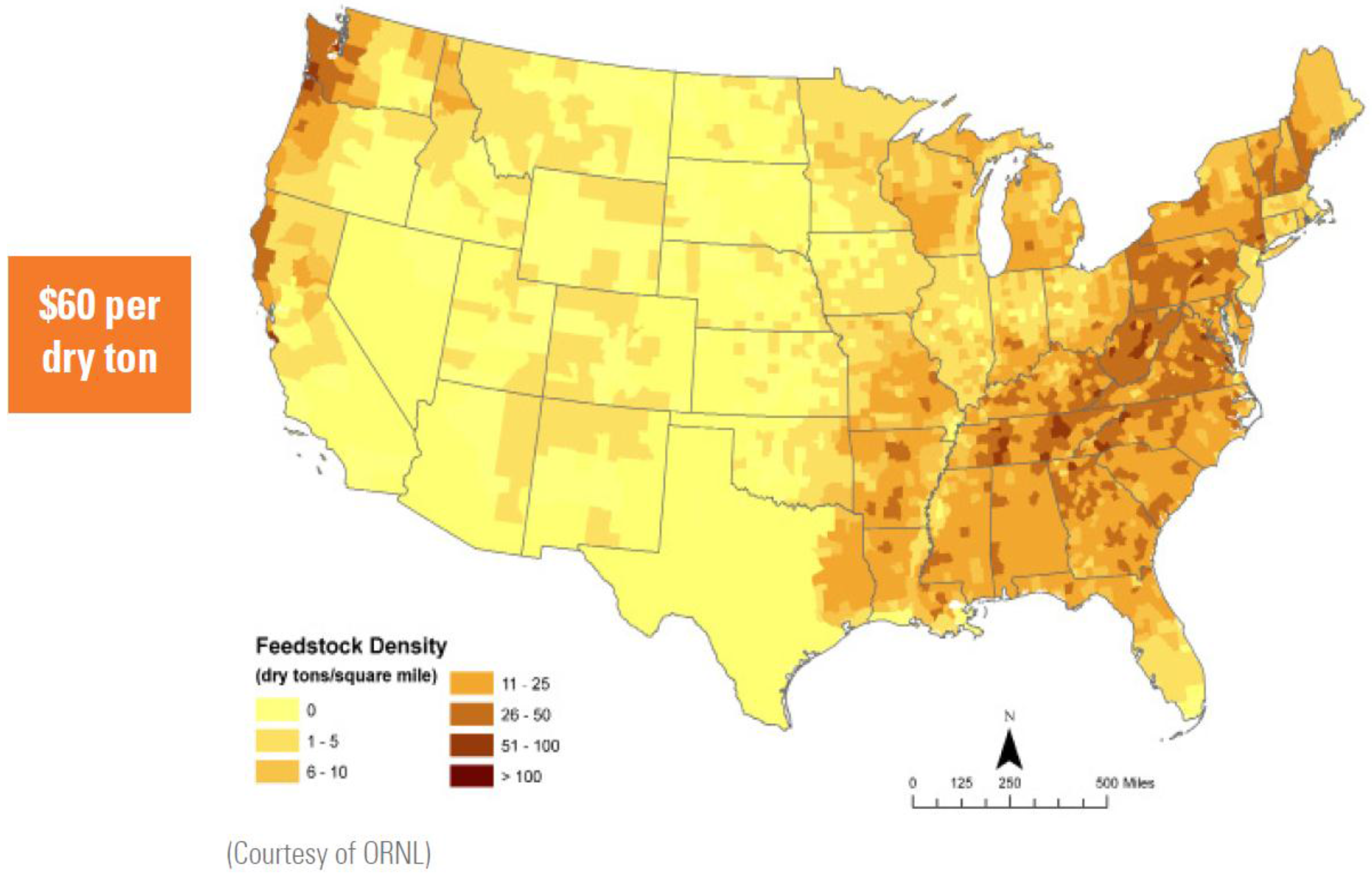
While energy crops (e.g., switchgrass) are expected to constitute the major portion of the biofuel feedstocks in 2022 and beyond, residues from the forest and the agricultural operations are critical feedstocks for the first-type generation of biofuel conversion facilities (e.g., corn-ethanol biorefineries). The report of the U.S. Department of Energy (DOE) “U.S. Billion-Ton Update: Biomass Supply for a Bioenergy and Bioproducts Industry” [10] projects that nearly 97 million dry tons of logging residues (unused portions of trees cut during logging) are currently available for bioenergy purposes. This makes up 38% of the 258 million dry tons of biomass that are available for new biofuel production. For example, as shown in Figure 1, logging residues are concentrated in the eastern and north western regions of the United States. In order to take advantage of such energetic potential, the design of efficient large-scale bioenergy SCs is required. Moreover, forest residues are low cost biomass sources; however, they also possess unfavorable quality characteristics, specially, the high ash content [11].

This paper addresses the problem of designing cost-effective bioenergy SCs by presenting a novel supply chain network design modeling approach that integrates the inherent costs associated to the quality of logging residues. Particularly, this research aims to amend the lack of theoretical background that directly hinders the design of robust biomass-to-biorefinery supply chains. It integrates the logging residues quality specifications needed by the conversion process and the impact of biomass quality characteristics on the supply chain network design. A special characteristic of the proposed computational and theoretical scheme is that it can be straightforwardly transferred to other types of biomass SCs and can also be transferred to other chemical and food industry SCs.

This paper is structured as follows: Section 2 presents a brief literature review of supply chain design, modeling and optimization; poor quality costing; and biofuel feedstock logistics models. Section 3 presents the novel modeling approach, named the Bioenergy Supply Chain including Quality (BioSC-Q) model, which is used to quantify the impact of quality control strategies implemented during collection, storage and transportation on the overall cost. Section 4 presents a realistic case study in the state of Tennessee and the analysis of the results employing the proposed framework. Section 5 presents a summary of the key insights and the concluding remarks, as well as recommendations for future work.

2. Literature Review

2.1. Quality Costing

The proposed model aims to quantify biomass quality costs and it is inspired in the accounting and quality management concept of the Cost of Quality (COQ). A brief review of the COQ or cost of poor quality models is presented in the following paragraphs. Joseph Juran´s [12] analogy of “Gold in the Mine” is defined as the “total of avoidable costs of quality.” According to Juran et al. [13], this concept suggests that costs resulting from defects were a gold mine in which lucrative digging could be done. Feigenbaum [14] developed the prevention-appraisal-failure (PAF) classification. The PAF classification offers specific advantages, such as its universal acceptance, identification of different types of expenditures, and provides a criterion to help determining whether specific costs can be classified as quality-related costs. The premise behind Feigenbaum’s classification [14] is that a company can reduce the quality-related costs by cutting the two major cost segments of quality (i.e., failures and appraisal costs) by means of much smaller increases in the prevention costs. The definitions for each of the categories of the PAF classification were defined by Campanella [15], and are summarized as follows:

-

Prevention costs are “the costs of all activities specifically designed to prevent poor quality in products and services.”

-

Appraisal costs are “the costs associated with measuring, evaluating, or auditing products or services to assure conformance to quality standards and performance requirements.”

-

Internal failure costs are “the costs resulting from products or services not conforming to requirements which occur prior to delivery or shipment to the customer.”

-

External failure costs are “the costs resulting from products or services not conforming to requirements which occur after delivery or shipment of the product, and during or after furnishing of a service to the customer.”

According to Porter and Rayner [16], the main assumptions of the PAF model are that (1) investments in appraisal will reduce failure costs and (2) further investments in prevention activities will also reduce failure costs. The PAF classification allows practitioners to identify quality-related costs and expresses each category in terms of percentages of the total cost (e.g., refer to Figure 2). Juran et al. [13] merged the Feigenbaum’s PAF concept with their original concepts, which resulted is what is known as the traditional COQ trade-off between the prevention, the appraisal and the failure costs. A variety of studies performed during the 1980´s demonstrated that the traditional COQ trade-off model of Juran was not completely valid. Schneiderman [17] affirmed that the minimum COQ could lie at 100% good products if the incremental cost of approaching a quality level of 100% is less than the incremental return from the improvement. In response, Juran and Gryna [18] revised the COQ trade-off between the prevention, the appraisal and the failure costs and eliminated the asymptotic behavior of the sum of the appraisal and the prevention costs. They asserted that 100% quality conformance might be reached for finite prevention and appraisal costs, considering the conditions of the twentieth century where a growth of the manufacturing and the automated inspection technologies occurred. Figure 2 compares the classical model with the updated model.

In this work, the following definition for the COQ across a supply chain is adopted: The sum of the costs incurred across a supply chain in preventing poor quality of product and/or service to the final consumer, the costs incurred to ensure and evaluate that the quality requirements are being met, and any other incurred as a result of poor quality [19].

2.2. Integrated Biofuels Supply Chain Modeling

Supply chain modeling aims to provide an optimal platform for the efficient and effective SC management by developing mathematical models and optimization methods that enhance the resource utilization. Supply chain modeling can be divided into three main decision timeframes: operational, tactical and strategic decisions (i.e., hourly and weekly, monthly and yearly decisions, respectively) and into three main SC levels: upstream (from farms, passing through storage facilities, to pre-processing facilities), midstream (related to the activities within biorefineries) and downstream (spanning from distribution centers to the customer service stations.)

An et al. [20] provided a comprehensive review of biofuel and petroleum-based fuel SC models. The downstream level is similar in the biofuel and the petroleum-based fuel SC; therefore, some practices and models can be adapted to address biofuel SC design problems. However, the upstream and the midstream levels are significantly different for the biofuel industry due to the biomass properties and conversion processes, among other things. An et al. [20] found that most of the research on biofuel SC modeling has been done for the upstream-operational level. Nonetheless, integrated frameworks for biofuel SC planning and design should have the capacity to (1) quantify the economic losses due to poor quality of the feedstock and (2) evaluate the impacts of investments on quality activities to improve the conversion throughput. Integrated SC modeling includes various strategic, tactical and operational decisions, in which, very often, several modules are interconnected.

Zhang et al. [21] formulated an optimization framework for switchgrass-based bioethanol SCs that aimed to minimize the total costs and determine the optimal SC/logistic decisions. The authors proposed an integrated mathematical model to determine the optimal overall SC/logistics decisions while considering existing constraints. Shabani and Sowlati [22], proposed a tactical SC design approach for conventional forest biomass power plants using a mixed integer non-linear programming (MINP) model. The model considers the biomass procurement, its storage, the energy production potential and the ash management. The authors established that the cost of generating energy from forest biomass is higher compared to other biomass sources due to various factors including the transportation costs and the quality of the raw material. They demonstrated that investments in the ash recovery systems have both economic and environmental benefits during the production of energy.

Regarding previous research employing multi-objective approaches in bioenergy SC modeling, Ayoub et al. [23] proposed an optimization framework for bioenergy SCs that simultaneously utilize a set of bio-resources from diverse nature and source (i.e., wet, dry, agricultural, and industrial residues, among others). The model considers four objectives simultaneously: (1) the minimization of the total costs; (2) the minimization of bioenergy emissions; (3) the minimization of the energy to produce bioenergy; and (4) the minimization or maximization of personnel hires. Bioenergy systems are labor-intensive projects, thus, the maximization of the personnel hires (i.e., the fourth performance measure) was due to the conditions of the case study, which considered data from the city of Lida in Japan, where the workforce is decreasing. Thus, the number of workers was considered as a design variable.

The quality of the raw materials and the quality of the final products have not been considered in the majority of the bioenergy SC frameworks. The seminal work by Gunnarsson et al. [24] consider a constraint for the maximum proportion of low quality biomass. Decision variables considered whether or not additional crop areas and sawmills have to be contracted, the flow of products from sawmills and import harbors, and the terminals to be used. A case study from Sweden is analyzed.

Castillo-Villar et al. [25,26,27] successfully integrated the cost of poor quality as an analytical expression within the supply chain modeling of manufacturing processes. No work has integrated the quality-related issues and costs within bioenergy supply chains. Hence, the research conducted by Castillo-Villar et al., within the manufacturing field serves as a foundation for the purposes of modeling the bioenergy supply chain.

From the previous literature review, it becomes evident the need for more scholarly work to extend, implement and apply the theoretical concept of cost of poor quality, that is, to define and model the cost of poor quality in the biomass-to-biorefinery supply chains. Thereby, this relevant need motivates this research, which ultimately proposes a complete scheme that integrates the applicable quality-related costs, as well as the traditional costs such as operational/logistic costs, into the SC design process. The challenge is to define the critical-to-quality characteristics (e.g., the ash and the moisture contents) and translate these characteristics into an analytical expression that conveys the cost of poor quality.

This paper proposes a Mixed Integer Quadratically Constraint Programming (MIQCP) model that minimizes the entire bioethanol SC costs, considering quality-related costs (BioSC-COQ). The BioSC-COQ model is unique in the sense that it incorporates the following characteristics:

• The BioSC-COQ model considers two quality characteristics: the moisture and the ash contents, which have not been considered in the literature. The inclusion is achieved through a quality costing classification of forest residues, where prevention, failure and opportunity costs are quantified across the SC.
• The BioSC-COQ model selects among different harvesting methods, which differ depending on the initial moisture contents. The selection of different harvesting methods directly impacts the transportation costs and the costs incurred to mechanically dry the biomass prior to the conversion process.
• The BioSC-COQ model selects the ash content, which in turn produces the minimum overall cost. A trade-off between the quality control activity to reduce ash and losses due to high ash content is modeled.

Noteworthy, the BioSC-COQ is a proof-of-concept novel model that aims to quantify biomass quality-related costs for the implementation of quality control activities and the impact of biomass quality on the supply chain design. This model is single objective, but can be extendable to a multi-criteria model that includes environmental objectives (as discussed in Section 7).

3. The BioSC-COQ Model Formulation

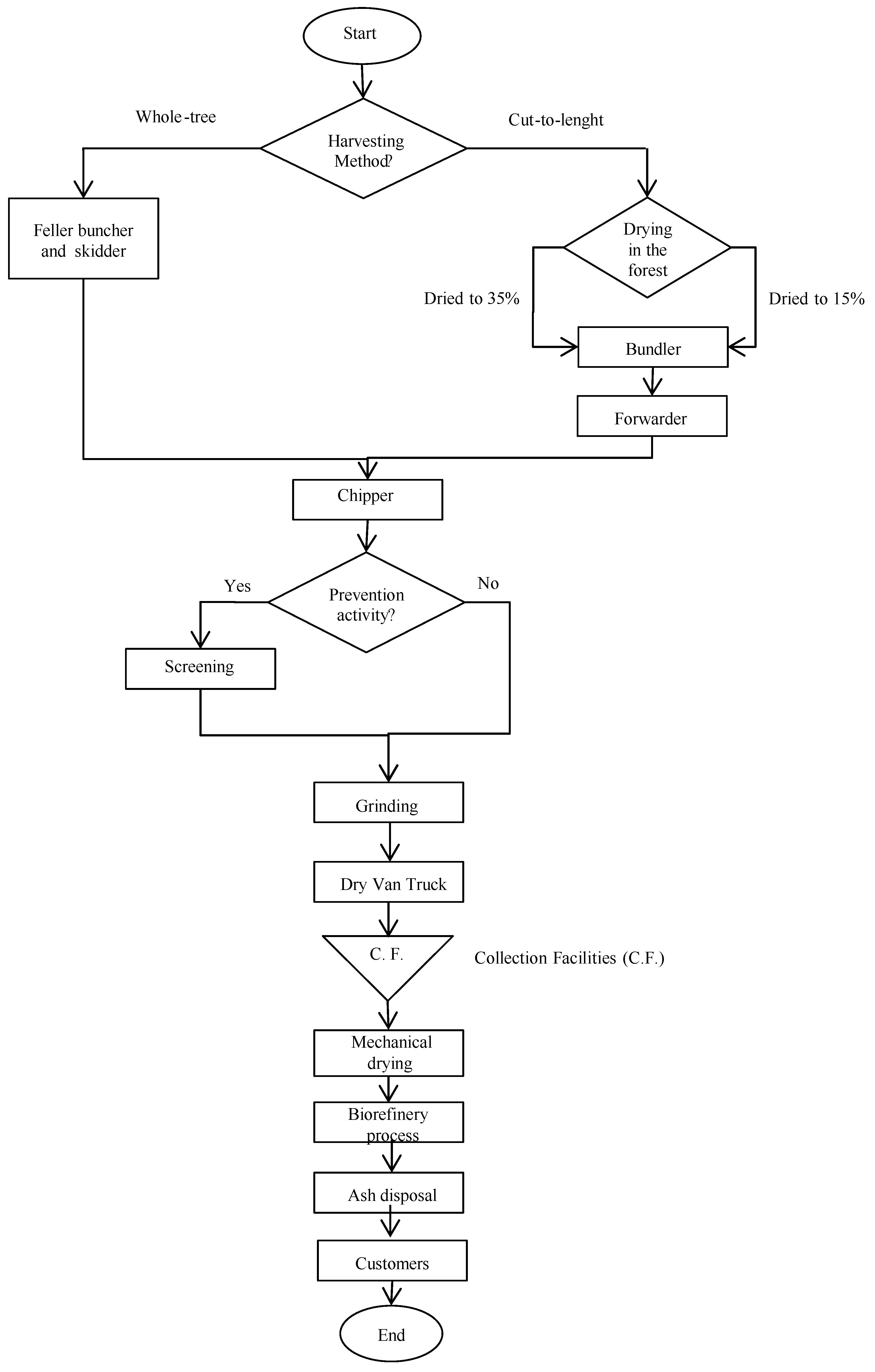
3.1. Harvesting Methods

Two collection strategies for logging residues are considered, as depicted in Figure 3; the whole-tree and cut-to-length harvesting methods. The whole-tree (WT) harvesting system uses a feller-buncher to fall and stack trees in the forest. A skidder collects the stacks of trees and hauls them to the landing. At the landing, a delimber removes the tops and branches from the trunk of the tree, which are to be sold for logs or pulpwood. The residues can be chipped for transportation to a biorefinery.

The cut-to-length (CTL) system consists of a specialized harvester that cuts the tree at the base. Then, it rotates the tree to a position parallel with the ground and pulls it through rollers that delimb the tree as it cuts the logs into customized lengths. The residues are typically left in the forest. If these residues are to be used for bioenergy production purposes, they can be left in the forest for several weeks or months to allow them to dry naturally as part of a moisture management strategy. After being allowed to dry, they are collected and transported to the landing for chipping and transport. Collecting and transporting loose residues can be a time-consuming and costly operation.

As with all woody biomass, the moisture and the ash contents are critical parameters while determining the efficiency of the conversion technologies (e.g., the yields and the feasibility to use as-is biomass). Woody biomass is best suited for thermo-chemical conversion processes, which require that feedstocks have moisture contents of 10% or less and ash contents of 1% or less (i.e., these represent the target values). Biomass with moisture and ash concentrations above these target values will incur additional costs within the SC.

Woody biomass entering a thermochemical conversion facility will undergo a process of mechanical drying (e.g., using a rotary drum dryer). The time spent in the dryer and the energy used by the dryer will depend on the initial moisture content. Allowing residues to dry in the forest (e.g., the CTL system) prior to the transportation to the biorefinery will reduce the energy required and, thus, the costs to dry the biomass. For the purposes of this study, it is assumed that the moisture content of the useful residues at the time a tree is cut is 50% (this corresponds to the WT system). After the residues are allowed to dry in the forest, the moisture content can be expected to be lower [28]. For this study, the CTL system can reach a 35 or 15% moisture content depending on the time the biomass is allowed to naturally dry in the forest.

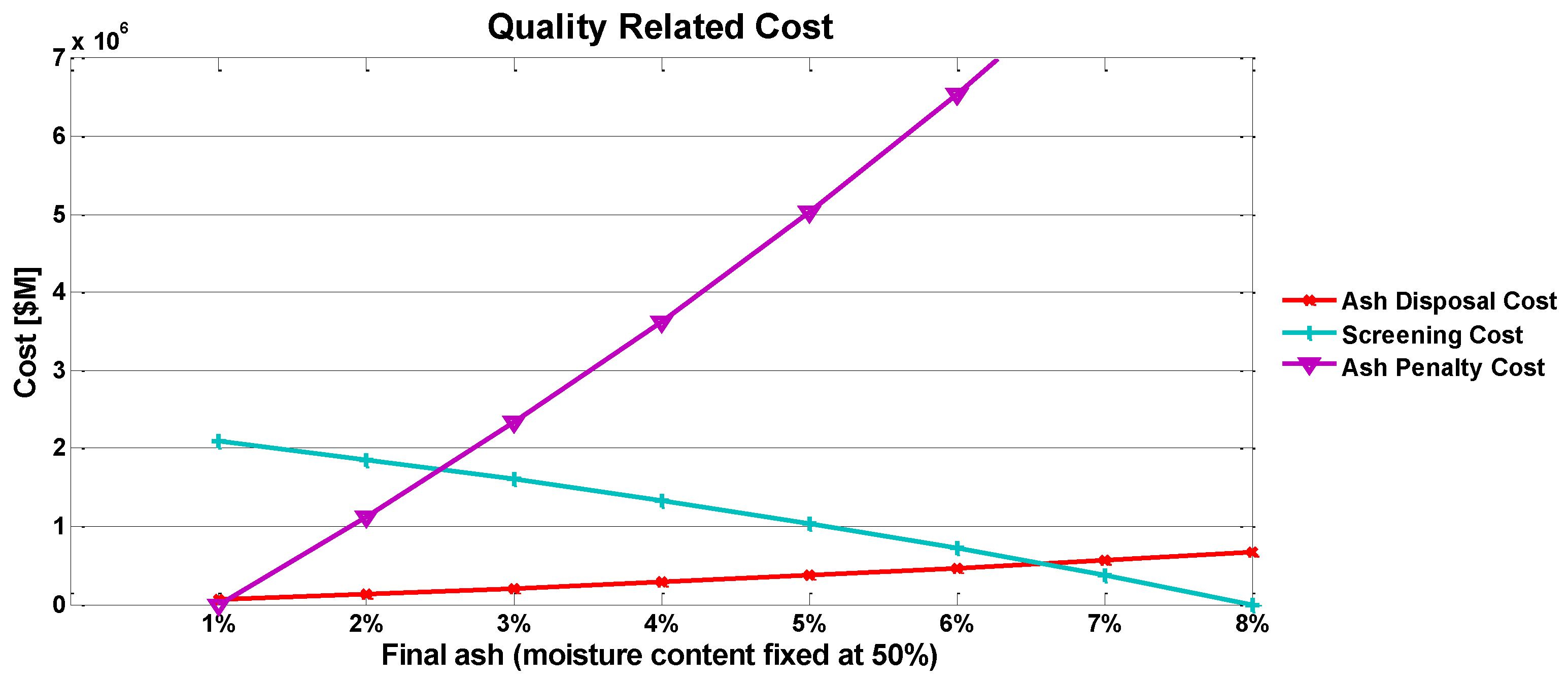
On the other hand, if the biomass contains more ash than the target content, the remaining ash will be left in the reactor; thus, it will require proper disposal. As expected, the cost associated with the ash disposal increases with increasing initial ash content. This study considers the beneficial effects of passing the biomass through a screener following grinding, as described by Dukes et al. [29], to separate ash from the woody biomass chips, as shown in Figure 3.

Table 1. Harvesting Methods.

Method	Description
P1	Whole-tree without screening
P2	Cut-to-Length without screening (dried to 15%)
P3	Cut-to-Length without screening (dried to 35%)
P4	Whole-tree with screening
P5	Cut-to-Length with screening (dried to 15%)
P6	Cut-to-Length with screening (dried to 35%)

shows the harvesting methods that are considered in this work, indicating the different moisture contents and which scenarios employ biomass screening as a prevention activity.

3.2. Quality Costing Model for the Logging Residues Supply Chain

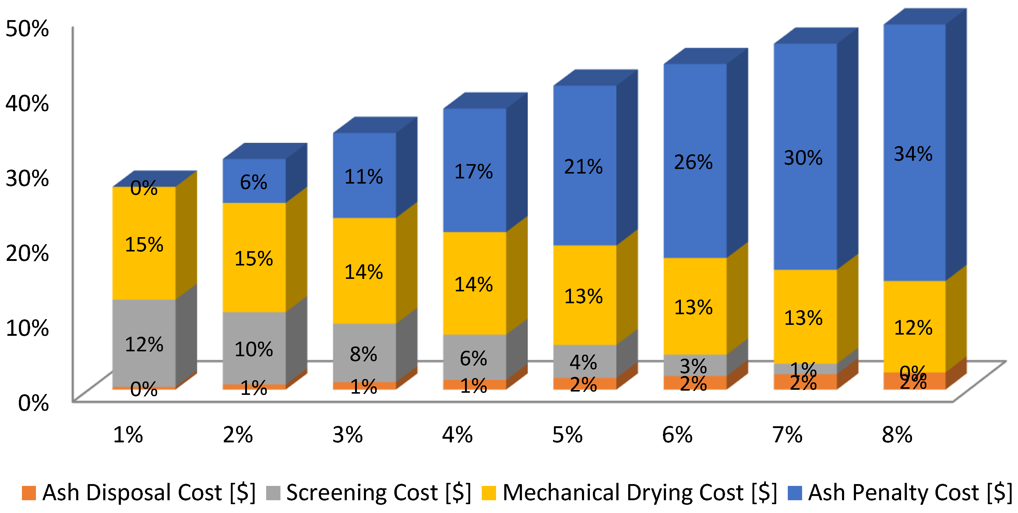
This section presents a formal methodology to compute the cost incurred by quality and operational affairs within the SC. The BioSC-COQ model defines as critical-to-quality characteristics the moisture and the ash contents. The costs include the fixed equivalent annual investment costs required to open collection facilities, the fixed equivalent annual investment costs required to open the bio-refineries, the mechanical drying, grinding, screening, ash disposal, ash penalty and the transportation costs. As mentioned in the background section, the total cost of poor quality can be broken into the conformance costs (prevention and appraisal categories) and the nonconformance costs (internal and external failure as well as opportunity costs). The definitions of these costs within the logging BioSC-COQ model are described as follows.

The conformance costs are linked to two prevention costs. The first prevention cost is related to the moisture content and consists of the collection cost after drying the useful residues. A benefit of implementing the CTL harvest strategy is the opportunity to naturally dry the biomass in the forest to reduce, to some extent (e.g., 35% or 15%), the initial moisture content (e.g., ~50%). Reducing the moisture content decreases the transportation cost as moist biomass is bulky and reduces the energy required during the mechanical drying process at the biorefinery. However, the additional costs of collecting the residues and transporting them to the landing are incurred. In the baseline WT system, the collection cost is null as all the collection costs are only attributed to conventional products (logs or pulpwood). The second prevention cost is related to the ash content and consists of the screening cost incurred in order to reduce the initial ash concentration. Passing the wood chips through a screener after grinding is considered in some harvesting methods (e.g., P1 and P4 in Table 1). It is worth noting that no inspection-related techniques (appraisal costs) are considered for this BioSC-COQ model because inspecting the quality of the biomass is not a common practice and inspection per se does improve the biomass quality.

The non-conformance costs are linked to the failure costs associated to biomass that does not meet the moisture and the ash contents specifications for the energy conversion process. Although the CTL harvest strategy incurs an additional cost for collecting residues as a separate operation, it reduces the energy required to dry woody biomass from a 35% or 15% to 10% moisture content (i.e., the target value required by the conversion process). The cost of the mechanical drying process is considered a nonconformance cost and it is directly related to the moisture content. Similarly, the cost to dispose the ash that remains in the reactor, after the conversion process takes place, is also a nonconformance cost that is directly associated to not having the target ash content before the biomass is left at the throat of the reactor.

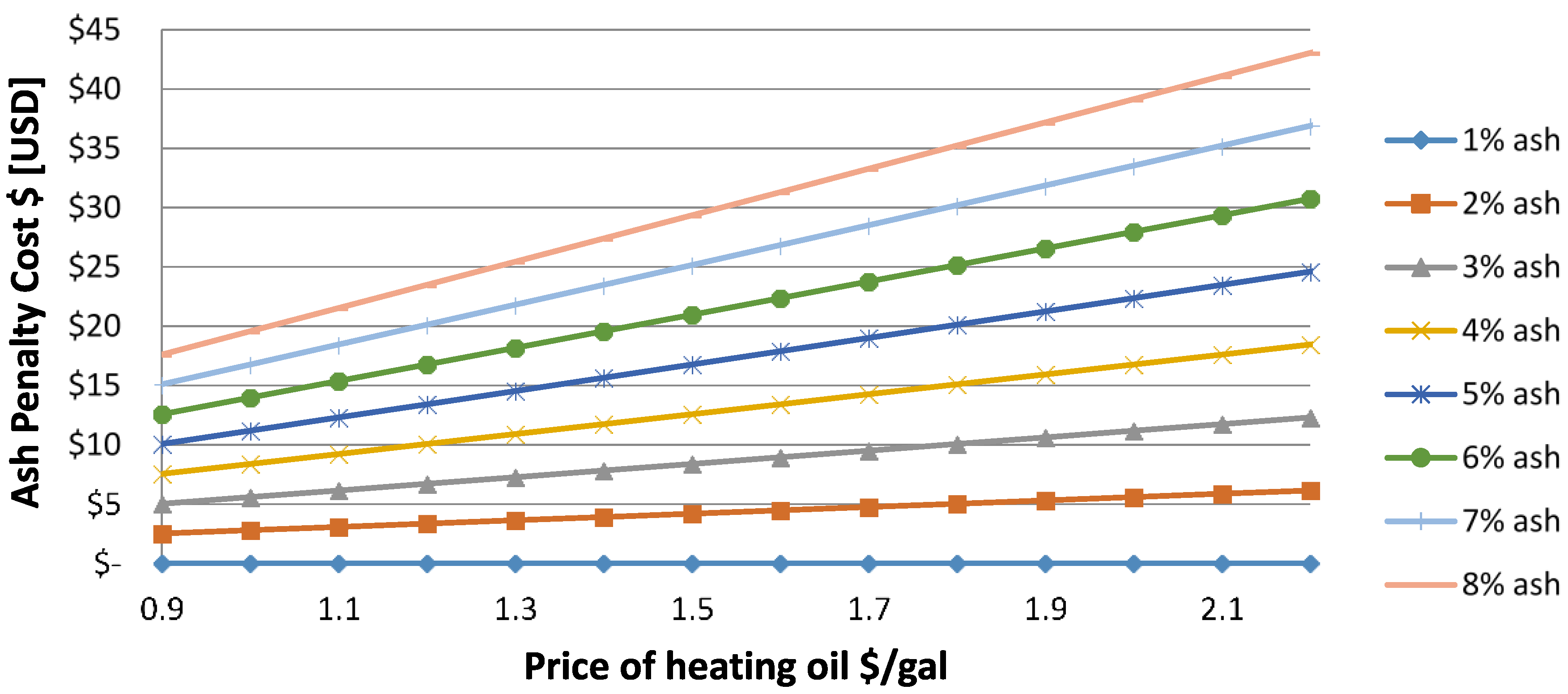
Moreover, the opportunity cost is modeled as the ash penalty cost for reduced oil yield. The difference between the profit that would have been generated when meeting the target ash content versus the yield obtained with a high ash content is computed.

All these quality-related costs are expressed in analytical expressions and integrated into the mathematical model presented in Section 3.3.

3.3. Mathematical Formulation

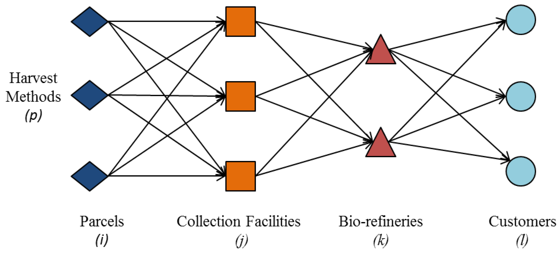
The bioenergy supply chain network modeled is depicted in Figure 4.

Indices/Sets

$I$	Set of parcels.
$J$	Set of potential sites for collection facilities.
$K$	Set of potential sites for bio-refineries.
$L$	Set of customers.
$P$	Set of harvesting methods.

Decision Variables

$x_{ijp}$	Amount of biomass [ton] harvested via method p, shipped from parcel i to the collection facility j, in period t, where $p\in P$, $i\in I$ and $j\in J.$
$y_{jkp}$	Amount of biomass [ton] harvested via method p, shipped from the collection facility j to the bio-refinery k, in period t, where $p\in P$, $j\in J$ and $k\in K.$
$z_{kl}$	Amount of biofuel [liters] shipped from bio-refinery k to customer l in period t, where $k\in K$ and $l\in L.$
$A_{ijp}$	Binary variable that is equal to 1 if parcel i connected to the collection facility j that uses the harvesting method p is active in period t, and equal to 0 otherwise.
$f_j$	Binary variable that is equal to 1 if collection facility j is open, and equal to 0 otherwise.
$g_k$	Binary variable that is equal to 1 if bio-refinery k is operating, and equal to 0 otherwise.
$F_1^{AH}$	Variable that establishes the final ash content, where $Ash\in \left(0.08, 0.07, \dots , 0.01\right)$.

Parameters

Operational Parameters

${\Omega }_i$	Maximum amount [tons] of available biomass in parcel I, where $i\in I$.
$M{P}_j$	Capacity of a collection facility [tons] j, where $j\in J$.
$M{C}_k$	Capacity of the bio-refinery [MLPY] k, where $k\in K$.
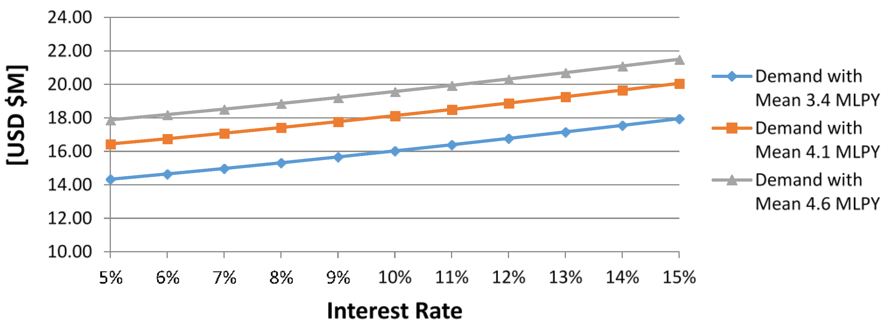
${\rho }_l$	Customer demand [MLPY] l, where $l\in L$.
$C{F}_j$	Fixed annual equivalent cost [USD $] for opening the collection facility j, where $j\in J$.
$C{B}_k$	Fixed annual equivalent fixed cost [USD $] for opening the bio-refinery k, where $k\in K$.
$W$	Number of bio-refineries k that can operate.
$M$	Very large positive value.
$S_p^2$	Grinding cost [USD $] employing harvesting method p, where $p\in P$.

Transportation Parameters

$C_{ijp}$	Transportation cost [USD $] per dry ton using harvesting method p from parcel i to collection facility j, where $p\in P$, $i\in I$ and $j\in J$.
$C_{jkp}$	Transportation cost [USD $] per dry ton using harvesting method p from collection facility j to bio-refinery k, where $p\in P$, $j\in J$ and $k\in K$.
$C_{kl}$	Transportation cost [USD $] per volume from bio-refinery k to the customer l, where $k\in K$ and $l\in L$.

Quality Parameters

$C{H}_{ip}$	Collection cost [USD $] per dry ton of feedstock harvested employing the method p, in parcel i, where $p\in P$ and $i\in I$.
$F_0^{AH}$	Parameter that establishes the initial content of ash, where $Ash\in \left(0.08, 0.07, \dots , 0.01\right)$.
$S_p^1$	Mechanical drying cost [USD $] employing harvesting method p, in period t, where $p\in P$.
$S{3}^{AH}$	Ash disposal cost [USD $], which is calculated from a linear regression such that $S{3}^{AH}=28.86F_1^{AH}$, where $Ash\in \left(0.08, 0.07, \dots , 0.01\right)$.
$S{4}^{AH}$	Ash penalty cost [USD $], which is calculated from a linear regression such that $S{4}^{AH}=492.66F_1^{AH}-4.9266$, where $Ash\in \left(0.08, 0.07, \dots , 0.01\right)$.
$S{5}^{AH}$	Screening cost [USD $], which is calculated from a linear regression such that $S{5}^{AH}=135\left(F_0^{AH}-F_1^{AH}\right)$, where $F_0^{AH}$ is the initial level of ash content, and $F_1^{AH}$ is the final level of ash content, where $Ash\in \left(0.08, 0.07, \dots , 0.01\right),$ with the conditional $F_1^{AH}\le F_0^{AH}$.
$S{6}^{AH}$	Oil yield [liters], which is calculated from a linear regression such that $S{6}^{AH}=-10507.4F_1^{AH}+324.69$, where $Ash\in \left(0.08, 0.07, \dots , 0.01\right)$.

Mathematical Model

The BioSC-COQ model aims to minimize overall costs, as follows:

$$\text{Min}\left[{\text{Obj}}_1=C{T}_o=CT+CH+CP+CB+MD+AS+SC+GR+AP\right]$$

(1)

where $CT$ [$] is the total cost of transportation, $CH$ [$] is the total cost of the harvest processes, $CP$ [$] is the fixed annual equivalent cost for opening the collection facilities, $CB$ [$] is the fixed annual equivalent cost for opening the bio-refineries, $MD$ [$] is the mechanical drying cost, $AS$ [$] is the ash disposal cost, $SC$ [$] is the screening cost, $GR$ [$] is the grinding cost and $AP$ [$] is a penalty cost for reduced oil yield due to high ash content. Each cost is modeled as follows:

$$CT={\displaystyle \sum }_{i=1}^I{\displaystyle \sum }_{j=1}^J{\displaystyle \sum }_{p=1}^P{C}_{ijp}{x}_{ijp}+{\displaystyle \sum }_{j=1}^J{\displaystyle \sum }_{k=1}^K{\displaystyle \sum }_{p=1}^P{C}_{jkp}{y}_{jkp}+{\displaystyle \sum }_{k=1}^K{\displaystyle \sum }_{l=1}^L{C}_{kl}{z}_{kl}$$

(2)

$$CH={\displaystyle \sum }_{i=1}^I{\displaystyle \sum }_{j=1}^J{\displaystyle \sum }_{p=1}^{P}C{H}_{ijp}{x}_{ijp}$$

(3)

$$CP={\displaystyle \sum }_{j=1}^{J}C{F}_j{f}_j$$

(4)

$$CB={\displaystyle \sum }_{k=1}^{K}C{B}_k{g}_k$$

(5)

$$MD={\displaystyle \sum }_{j=1}^J{\displaystyle \sum }_{k=1}^K{\displaystyle \sum }_{p=1}^P{S}_p^1{y}_{jkp}$$

(6)

$$AS={\displaystyle \sum }_{j=1}^J{\displaystyle \sum }_{k=1}^K{\displaystyle \sum }_{p=1}^{P}S{3}^{AH}{y}_{jkp}$$

(7)

$$SC={\displaystyle \sum }_{i=1}^I{\displaystyle \sum }_{j=1}^J{\displaystyle \sum }_{p=1}^{P}S{5}^{AH}{x}_{ijp}$$

(8)

$$GR={\displaystyle \sum }_{i=1}^I{\displaystyle \sum }_{j=1}^J{\displaystyle \sum }_{p=1}^P{S}_p^2{x}_{ijp}$$

(9)

$$AP={\displaystyle \sum }_{j=1}^J{\displaystyle \sum }_{k=1}^K{\displaystyle \sum }_{p=1}^{P}S{4}^{AH}{y}_{jkp}$$

(10)

The BioSC-COQ model is subject to the following constraints:

$${\displaystyle \sum }_{j=1}^J{\displaystyle \sum }_{p=1}^P{x}_{ijp}\le {\Omega }_i\forall i\in I$$

(11)

Constraints Equation (11) impede to exceed the capacity of each parcel i:

$${\displaystyle \sum }_{i=1}^I{\displaystyle \sum }_{p=1}^P{x}_{ijp}\le M{P}_{jt}{f}_j\forall j\in J$$

(12)

Constraints Equation (12) limit the capacity of each collection facility j:

$${\displaystyle \sum }_{l=1}^L{z}_{kl}\le M{C}_k{g}_k\forall k\in K$$

(13)

Constraints Equation (13) impede to exceed the capacity of each bio-refinery k:

$${\displaystyle \sum }_{k=1}^K{z}_{kl}={\rho }_l\forall l\in L$$

(14)

Constraints Equation (14) ensure demand satisfaction for each customer l:

$${\displaystyle \sum }_{i=1}^I{\displaystyle \sum }_{j=1}^J{x}_{ijp}-{\displaystyle \sum }_{j=1}^J{\displaystyle \sum }_{k=1}^K{y}_{jkp}=0\forall j\in J, \forall p\in P$$

(15)

Constraints Equation (15) allow the balance of flow between the parcel i and the facility j, and between the facility j and the bio-refinery k:

$${\displaystyle \sum }_{j=1}^J{\displaystyle \sum }_{k=1}^K{\displaystyle \sum }_{p=1}^{P}S{6}^{AH}{y}_{jkp}-{\displaystyle \sum }_{k=1}^K{\displaystyle \sum }_{l=1}^L{z}_{kl}=0\forall k\in K$$

(16)

Constraints Equation (16) allow the balance of flow between the facility j and the bio-refinery k, and between the bio-refinery k and the customer l:

$$x_{ijp}-M{A}_{ijp}\le 0\forall i\in I, \forall j\in J, \forall p\in P$$

(17)

Constraints Equation(17) ensure that biomass shipment can only be done through active parcels $i\in I$:

$${\displaystyle \sum }_{j=1}^J{\displaystyle \sum }_{p=1}^P{A}_{ijp}=1\forall i\in I$$

(18)

Constraints Equation (18) ensure that only one harvesting method p can be employed at each parcel i:

$${\displaystyle \sum }_{k=1}^K{g}_k\le W$$

(19)

Constraints Equation (21) establish the maximum number of biorefineries that can operate:

$$x_{ijp}\ge 0y_{jkp}\ge 0z_{kl}\ge 0\forall i\in I,\forall j\in J,\forall k\in K,\forall p\in P$$

(20)

$$A_{ijpt}\in \left\{1,0\right\}{f}_j\in \left\{1,0\right\}{g}_k\in \left\{1,0\right\}\forall i\in I,\forall j\in J,\forall k\in K$$

(21)

$$F_1^{AH}\in \left\{0.01,\dots ,0.08\right\}$$

(22)

Constraints Equations (20)–(22) define the type of the decision variables in the model.

4. Case Study

A realistic case study is presented to test the BioSC-COQ model; the input parameters are shown in

Table A1. List of input parameters for the BioSC-COQ model.

Source	Input Parameter	Value
Operational Parameters
[30]	Available biomass.	Ωi = According to Equation (26) and Table A2 in Appendix (∀i).
[41]	Capacity of collection facilities.	MPj = [110,000; 200,000; 300,600] Ton (∀j).
[21]	Capacity of bio-refineries.	MCk = [190, 380] MLPY (∀k).
[32]	Demand from customers.	rl = demand follows a normal distribution with a standard deviation of 15% from the mean.
[41]	Fixed equivalent annual cost (EAC) for opening collection facilities.	CFj = [399,404; 718,927; 1,038,450] (∀j).
[21]	Fixed equivalent annual cost (EAC) for bio-refineries of 190 MLPY.	CBk = 6,230,696 (∀k).
[21]	Fixed equivalent annual cost (EAC) cost for bio-refineries of 380 MLPY.	CBk = 11,502,825 (∀k).
[10]	Cost of grinding ($/dry ton).	S2p = 13.00 (∀p).
Transportation Parameters
[37]	Transportation cost per dry ton.	Cijp = Refer to Section 3 (∀p, i, j).
[37]	Transportation cost per dry ton using harvest method p.	Cjkp = Refer to Section 3 (∀p, j, k).
[42]	Bioethanol transportation cost from k to l ($/km).	Ckl = 0.000028 (∀k, l, t).
Quality Parameters
[34]	Cost of the mechanical drying.	S1p = Refer to Section 3 (∀p).
[7]	Cost of ash disposal.	S3AH = Refer to Section 3
INL Thermochemical Design, based on data in [35]	Cost of ash penalty.	S4AH = Refer to Section 3
[29]	Cost of screening.	S5AH = Refer to Section 3
INL Thermochemical Design, based on data in [35]	Yield of biomass.	S6AH = Refer to Section 3 (∀p, i).
[33]	Collection Cost ($/dry ton).	Chip =11.25 (∀p, i).

in the Appendix and discussed in this section. The supply chain consists of three potential collection facilities, two potential biorefineries and twenty customers.

4.1. Operational Parameters

We consider data of the availability of logging residues in the region of Tennessee in the United States, including a few adjacent counties in the states of Kentucky, Virginia, North Carolina, Alabama, Mississippi, Arkansas and Missouri. A total of ninety nine counties were considered in this study, as shown in

Table A2. List of counties included in the case study.

County	Thousand Dry Tons/Yr	County	Thousand Dry Tons/Yr	County	Thousand Dry Tons/Yr
Alcorn	1080.9	DeSoto	196.95	Lawrence	2702.1
Allen	2403.4	Dickson	1674.8	Lewis	5505.3
Anderson	1208.2	Dyer	334.94	Limestone	668.8
Ashe	2276.2	Fayette	644.33	Lincoln	832.03
Bedford	303.44	Fentress	1163.6	Logan	871.65
Bell	1521.5	Franklin	1534.9	Loudon	200.43
Benton	653.24	Gibson	332.81	Macon	1175.4
Benton	1016.6	Giles	2365.2	Macon	1936.4
Bledsoe	2123	Graham	629.7	Madison	1103.3
Blount	413.95	Grainger	815.52	Madison	1193.5
Bradley	1069.8	Greene	451.34	Madison	1816.6
Buncombe	1530.2	Grundy	3219.1	Marion	2013.9
Calloway	976.41	Hamblen	117.64	Marshall	1453.7
Campbell	2285.1	Hamilton	1341.5	Marshall	197.07
Cannon	526.1	Hancock	396.49	Maury	675.99
Carroll	1835.1	Hardeman	3395.8	McCreary	1415.9
Carter	325.2	Hardin	5323.5	McMinn	2370.3
Cheatham	754.42	Hawkins	976.49	McNairy	4228.9
Cherokee	2065	Haywood	2369.7	Meigs	360.4
Chester	2128.3	Haywood	305.98	Mitchell	845.59
Christian	2757.5	Henderson	1271.3	Monroe	2019
Claiborne	1451.2	Henderson	1927.1	Monroe	1755.2
Clay	734.9	Henry	1429	Montgomery	799.36
Clay	568.15	Hickman	3202.1	Simpson	28.481
Clinton	1318.5	Houston	2847	Swain	430.99
Cocke	705.36	Humphreys	2542.3	Tippah	2022
Coffee	508.47	Jackson	5090.1	Tishomingo	3158.7
Crittenden	47.35	Jackson	4100.8	Todd	902.08
Cumberland	5840.5	Jackson	1274.9	Transylvania	137.39
Cumberland	2958.3	Jefferson	174.55	Trigg	2150.9
Davidson	54.19	Johnson	470.21	Wayne	1508.2
Decatur	2212.4	Knox	346.14	Whitley	2930.5
DeKalb	598.05	Lauderdale	1577.4	Yancey	760.85

. The availability of biomass (at the county level) is retrieved from the National Renewable Energy Laboratory’s (NREL) website [30]. The average annual forest residues are 300,530 dry tons.

In practice, the moisture content in the biomass is determined by several factors such as the weather conditions, the storage duration and the management practices. Equation (26) is used to estimate the moist biomass available:

$${\Omega }_i=\left(\frac{Dr{y}_{Ton}}{1-mc}\right)$$

(23)

where ${\Omega }_i$ [tons] is the weight of the moist biomass, mc [%] is initial moisture content (i.e., 50% is the baseline scenario in this case study) and $Dr{y}_{Ton}$ [tons] is the weight of the dry biomass (as shown in Table A2).

The equivalent annual cost (EAC) for opening the biorefineries (CB_k) is calculated in this study assuming a project life of 20 years and an interest rate of 15% [31]. The equivalent annual cost method is used to provide the annual cost incurred due to the net present value (NPV) of $39 million and $72 million corresponding to biorefineries of 190 and 380 MLPY, respectively [21]. Similarly, the equivalent annual investment costs for opening and operating the collection facilities is computed considering 20 years and an interest rate of 15% [31]; the net present value (NPV) of $2.5, $4.5 and $6.5 million associated with a capacity of 110,000, 200,000 and 300,600, respectively is used for the collection facilities [21]. The demand is assumed to follow a normal distribution with mean 3.4 [MLPY] and a standard deviation of 15% from the mean [32]. Finally, the cost of grinding is $13/dry ton [10].

4.2. Quality Parameters

A description of the quality-related input parameters follows. The conformance costs are the sum of (1) the collection cost after drying the biomass and (2) the screening cost. The CTL harvesting method provides the flexibility of drying the biomass naturally in the field; however, an additional collection cost is incurred by the biorefinery. The collection costs, which include collecting the residues and transporting them to the landing, is estimated as $11.25/dry ton [33]. As stated previously, allowing the biomass to dry in the forest reduces the moisture content from 50% to up to 15% (possibly in some, but not all, locations and seasons). In the WT harvesting method (with residues chipped at landing), the collection cost is assumed null as all collection costs are attributed to the conventional products (logs or pulpwood).

The screening cost is computed as a function of the amount of ash to be removed and is based on costs reported by Dukes et al. [29]. The initial ash concentration ($F_0^{AH}$) is assumed to be 8%. The ash screening costs ranged from $2.70/dry ton up to $9.45/dry ton for final ash contents of 6% and 1%, respectively. Based on these cost figures, a linear regression equation was fitted, that is, $S{5}^{AH}=135(F_0^{AH}-F_1^{AH})$, as shown in Section 3.3.

The non-conformance costs consist of the sum of: (1) the drying cost; (2) the ash disposal cost and (3) the ash penalization cost. The mechanical drying cost ($S_p^1$) is based on the estimates reported by Mani et al. [34]. Their analysis estimated a fixed cost of $2.46 for drying biomass. Additionally, the report estimates an operating cost of $7.84/dry ton for biomass with 40% moisture content. Using these cost figures as baseline, the cost for mechanically drying biomass was computed as $12.26, $9.32, and $5.40 per dry ton of biomass delivered to the biorefinery at 50%, 35% and 15% moisture contents, respectively.

The cost to dispose the ash that remains in the reactor after the energy conversion process takes place was derived from the results provided by Humbird et al. [7]. They estimated a total cost of $28.86 per ton of ash disposed. Using this value, the ash disposal cost estimates ranged from $0.29 to $2.31 for ash concentrations from 1% to 8%. The equation used to compute the ash disposal costs as a function of the final ash content is $S{3}^{AH}=28.86 F_1^{AH}$.

The ash content produces a significant impact on the yield of pyrolysis oil [11]. A linear relationship between the ash content and the percentage of oil yield was obtained from the data reported by Fahmi et al. [35]; we consider a baseline yield of 315.67 liters/dry ton with 1% ash. Then, we fitted a linear regression equation for predicting the oil yield (liters/dry ton) as: $S{6}^{AH}=-10507.4F_1^{AH}+324.69$. In order to quantify the monetary losses due to high ash concentrations, the price of No. 2 heating oil as of June 2015 (i.e., $0.4683/liter of oil) is used as a proxy of pyrolysis oil [36]. The ash penalty cost is applied to biomass that exhibited ash concentrations exceeding the desired value of 1% (i.e., the specification for thermochemical processes). The penalty cost is calculated as the difference between the profit made from selling the oil produced from feedstock with an ash concentration of 1% and the profit made from selling the oil produced from feedstock with higher ash concentrations. The higher the ash content, the lower the oil yield and the higher the economic loss. The prediction of this cost is performed through the following linear regression: $S{4}^{AH}=492.66F_1^{AH}-4.9266$.

4.3. Transportation Parameters

In order to compute the transportation costs, we used the equation proposed by Abbas et al. [37], $C_{ijp}=3.85+0.085\left(d_{ijp}\right)$ and $C_{jkp}=3.85+0.085\left(d_{jkp}\right)$ where $d_{ijp}$ is the distance from supplier $i$ to collection facility $j$ using method $p$ and $d_{jkp}$ represents the distance from collection facility $j$ to bio-refinery $k$ using method $p$. Since the baseline moisture content is assumed to be 50% (i.e., Whole-Tree scenario), the amount of biomass shipped ($x_{ijp})$ needs to be adjusted for the CTL scenarios where the biomass was naturally dried to 15% or 35% since the moisture content at the time of collection affects the transportation costs $\left(CT\right)$ as well as the cost of mechanically drying the biomass ($S_p^1$) to meet the conversion technology specifications. Thus, the transportation costs for CTL harvesting methods (i.e., P2, P3, P5, P6) are computed as $C_{ijp}=3.85+0.085\left(d_{ijp}\right)\left(1-mc\right)$ and $C_{jkp}=3.85+0.085\left(d_{jkp}\right)\left(1-mc\right)$ where $mc$ indicates the moisture content. The bioethanol transportation cost $(C_{kl})$ is estimated at $0.000028/km.

5. Computational Results

The computational experiments were conducted in a workstation with an Intel^® Xenon^® X5550 processor that operates at 2.67 GHz and with 4 GB of RAM. The implementation of the models was performed in GAMS 12 and solved with CPLEX 23.6.2 [38]. The implementation calls a mixed integer quadratically constrained programming (MIQCP) solver since the BioSC-COQ model is quadratic and contains design variables of integer-binary type.

5.1. Case Study Results

Table 2. Summary of the computational results (the annual costs are in USD). Optimal solution is in bold numbers.

Final Ash Content [%]	1%	2%	3%	4%	5%	6%	7%	8%
Final Moisture Content [%]	50%	50%	50%	50%	50%	50%	50%	50%
Biomass used (Dry tons)	220,944	228,588	236,781	245,583	255,064	265,308	276,408	288,477
Processing time [CPU sec]	1.37	0.91	0.87	0.90	0.83	0.89	0.83	0.78
Cost of Transportation [$/year]	2,951,344	3,052,446	3,160,795	3,277,200	3,402,592	3,538,056	3,684,856	3,844,475
Collection Cost [$/year]	0	0	0	0			0	0
Cost for Opening the Collection Facilities [$/year]	1,038,450	1,038,450	1,038,450	1,038,450	1,038,450	1,038,450	1,038,450	1,038,450
Cost for opening and operation the Biorefineries [$/year]	6,230,697	6,230,697	6,230,697	6,230,697	6,230,697	6,230,697	6,230,697	6,230,697
Ash Disposal Cost [$/year]	63,764	131,941	205,005	283,501	368,058	459,406	558,399	666,036
Screening Cost [$/year]	2,087,917	1,851,566	1,598,273	1,326,148	1,033,011	716,330	373,150	0
Grinding Cost [$/year]	2,872,267	2,971,649	3,078,155	3,192,579	3,315,838	3,448,998	3,593,299	3,750,203
Mechanical Drying Cost [$/year]	2,708,769	2,802,494	2,902,937	3,010,847	3,127,091	3,252,670	3,388,758	3,536,730
Ash Penalty Cost [$/year]	0	1,126,164	2,333,052	3,629,668	5,026,403	6,535,320	8,170,500	9,948,482
Performance Measure (Total Cost) [$/year]	17,953,208	19,205,406	20,547,363	21,989,090	23,542,140	25,219,928	27,038,108	29,015,073

(second column) summarizes the results of the case study. The breakdown of the overall cost consists of costs associated with the biomass quality control activities, including both the initial and the final ash and moisture contents, as well as operational and transportation costs. Moreover, the computational effort to achieve the results (in CPU seconds) is presented as well as the biomass utilized.

The initial ash content is 8% and the initial moisture content is 50%. The optimization algorithm selects the harvesting method, and consequently the final moisture content, as well as the ash level that minimizes the overall cost.

The optimal solution is shown in the second column in Table 2. The first finding is that the selected harvesting method is P4 (Whole-tree with screening, which has 50% moisture content). The second finding is that the optimized final ash content is 1%, which indicates that investing in preventive activities to reduce the ash content before reaching the throat of the reactor is more cost-effective than allowing the biomass to have an ash content higher than the specification at the conversion phase and, next, applying remedial activities such as the ash disposal and penalization for reduced yield.

Columns 3–9 in Table 2 illustrate the impact of changing the ash content lower limit. The original interval for the final ash content is from 1% to 8% and the optimal ash content is the minimum value (i.e., 1%). Columns 3–9 shown the impact of different minimum final ash contents (i.e., 2%, 3%, …, 8%) in the cost structure. The following remarks can be made. Firstly, as the ash content increases, more biomass is needed to meet the demand. This is due to the fact that high ash content reduces the oil yield; thus, more biomass is needed to meet the demand. More biomass increases the transportation, grinding and drying costs in 30% when comparing costs incurred with 8% versus 1% concentrations. Secondly, the ash disposal cost is 10 times higher if the final ash content is left at 8%. Similarly, the ash penalty cost considerably increases when the final ash content is left at 8% (from $0 to 45% of the total cost). If we compare the ash-related nonconformance costs (i.e., ash disposal and ash penalty) with the preventive or conformance costs (i.e., screening cost) incurred when reaching a final ash content of 1%, the screening cost needed to reduce the ash content to 1% represents only 15% of the total cost. Hence, prevention activities are cost-effective and ash quality control activities are recommended to reduce the nonconformance quality-related costs.

5.2. Quality-related Costs Analysis

Figure 5 depicts the trade-off curves of the ash quality-related costs at different levels of final ash content while considering the harvest method that minimizes the overall cost (i.e., Whole-Tree with 50% final moisture content). The conformance cost represented by the screening cost shows a decreasing behavior and reaches zero at 8% of ash. Contrary, the nonconformance costs linked to the ash disposal and ash penalty costs show an increasing behavior; specially, the ash penalty increases considerably when the ash content increases. Interestingly, Figure 5 shows that the conformance and nonconformance cost are balanced in between 2% and 3% ash. This represents the optimal COQ ash level (only considering the quality-related costs for ash). Above this point, the ash-related nonconformance costs increase substantially due to the losses caused by a reduced yield of oil. If the ash penalty is not considered in the analysis, the screening and the ash disposal costs would balance between 6% and 7% ash and this ash level would be the optimal COQ point.

It is worth noting that, with any final ash content from 1% to 8%, the model selects the method P4 Whole-tree harvesting without screening, with a final moisture content of 50%.

Figure 6 illustrates the COQ trade-off related to the moisture content for different harvesting methods. The selection of the harvesting method impacts the final moisture content of the logging residues, as indicated in the $x$ axis. The collection cost only applies for the CTL methods (which achieve lower moisture contents) and the drying costs decrease as moisture content decreases. The ash level was kept at 1% in the results shown in Figure 6. As discussed above, the optimal solution is to select the WT method at 50% moisture content (refer to Table 2) because the BioSC-COQ model optimizes both the ash and moisture contents that minimize the overall cost (i.e., fixed, operational, transportation and quality costs).

The results showed that the ash and moisture contents of logging residues affect the performance of the supply chain in monetary terms. Higher-than-target moisture and ash contents incur in additional quality-related costs. These costs are hidden in traditional supply chain network design models. Figure 7 depicts the contribution of the quality-related costs to the overall supply chain cost for different final ash contents while keeping the selected harvesting method (P4). The quality-related costs account for 27% of overall supply chain cost in the optimal solution. In contrast, the quality-related represent up to 49% of the overall supply chain cost if the final ash content is kept at 8%.

Figure 8 breaks down all the quality-related costs shown in Figure 7. For instance, the 27% corresponding to the first bar in Figure 7 can be broken down into 15% and 12%, associated with drying and screening costs, respectively. The trade-offs between the screening and the ash penalty costs represent the biggest change as the ash content increases. Particularly, the ash penalty cost is the biggest contributor to the quality-related costs and it goes from 0% (for 1% ash content) to 34% (for 8% ash content).

5.3. Sensitivity Analysis

Eleven interest rate cases are investigated to understand the impact on the fixed annual equivalent cost for opening the collection facilities ($C{F}_j$) and the biorefineries ($C{B}_k$). From Figure 9, it can be observed that the impact of changing the interest rate from 5% to 15% increases the total supply chain cost in around $3.6M. This change represents about 20% of the total cost of the original case study. Figure 9 also investigates the impact of changing the customer demand from a normally distributed demand with mean 3.4 MLPY with standard deviation of 15% to a normally distributed demand with mean 4.6 MLPY with standard deviation of 15%. In the optimized solution, the same collection facilities and biorefineries are selected; however, the total cost is increased in $3.5M when compared to the demand with mean of 3.4 MLPY.

We also investigate the impact of the price of oil on the ash penalty costs for reduced yield. Figure 10 shows a sensitivity analysis for prices starting from $0.9/gal (minimum price since 2010) to $2.2/gal. Higher slopes of ash penalty cost occur with final ash contents above 4%. In the extreme case of 8% final ash content, the penalty costs vary from $17.61 to $43.06. The proposed BioSC-COQ model selects the lowest final ash content (i.e., 1%); therefore, the ash penalty cost is zero and this parameter does not affect the optimal solution or the conclusion drawn from the numerical example.

6. Conclusions

A cost classification for quality-related costs in bioenergy supply chains using logging residues and a method to quantitatively incorporate the Cost of Quality (COQ) into a holistic supply chain model are presented in this paper. The proposed BioSC-COQ model selects the optimal final moisture and ash contents that minimize the overall cost within the supply chain by balancing the conformance (preventive) and nonconformance (reactive) quality control activities/losses. Furthermore, it includes traditional costs in supply chains such as logistic costs and operational costs of collection centers and bio-refineries while integrating a novel method of quantifying feedstock quality-related costs and selecting cost-effective quality control activities.

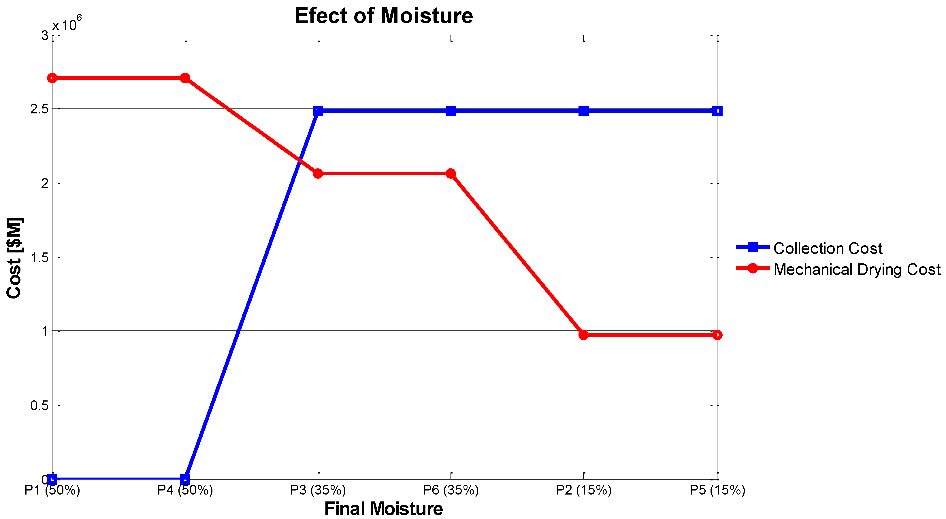
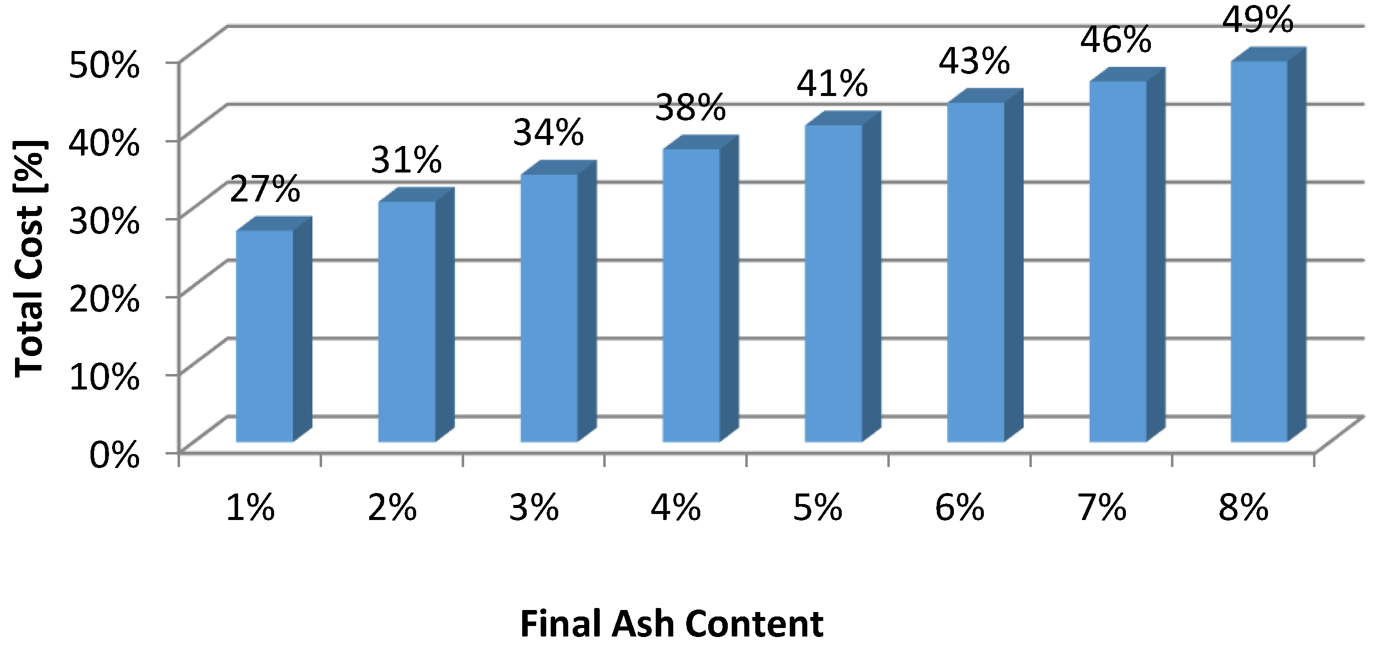
Based on the numeral experimentation, the total supply chain cost increased 7%, for each additional percent in the final ash content. Higher final ash contents result in a lower fuel production; therefore, greater amount of biomass is required to meet the customer demands. With each unit percentage increase of the final ash content from target value, oil yield decreased by 3.8% on average. Moreover, an ash content greater than the target value increases the overall cost by incurring in losses (i.e., ash penalty and ash disposal).

Regarding the impact of moisture content, the model selects the Whole-Tree harvesting method to reach a final moisture content of 50%. The moisture content in the logging residues increases the transportation and mechanical drying costs. However, the cost of collection (incurred when the biomass is left to dry) is higher than the mechanical drying and transportation costs.

In summary, this paper presents a model and solution approach that can be used as a decision support tool for the strategic and tactical planning and management of the logging residues supply chain network. The model takes into consideration aspects related to the biomass quality such as its ash and moisture contents (critical-to-quality characteristics). Previous works have acknowledged the importance of biomass quality in the decision making process but have not incorporated it into an analytical model that can serve as a decision support system. The proposed model closes this gap by building a more comprehensive model that considers and quantifies the feedstock quality implications.

7. Future Work

Future lines of research include, firstly, expanding this model to a stochastic programming model. For instance, weather conditions can be treated as a stochastic factor that could affect the initial moisture content. Secondly, this model is a single objective model; additional performance metrics can be considered. Some examples of alternative metrics include, but are not limited to: environmental objectives (e.g., minimize the impact of social footprint) and social objectives (e.g., maximize the jobs created by the project) [39]. Thirdly, this model considers the production of biofuels from a single type of biomass, future work might involve to model a mix of different types of biomass for the production of biofuels [5,40]. Thus, a natural extension of our work is to study the effect of ash and moisture content of various types of biomass. Fourth, an in-depth study of the effects of storage of biomass in the collection facilities and how storage affects the moisture content and the quality-related costs as well as the identification of optimal inventory management policies of the supply chain can be investigated as future work.