The Behaviour of Fracture Growth in Sedimentary Rocks: A Numerical Study Based on Hydraulic Fracturing Processes

Abstract

To capture the hydraulic fractures in heterogeneous and layered rocks, a numerical code that can consider the coupled effects of fluid flow, damage, and stress field in rocks is presented. Based on the characteristics of a typical thin and inter-bedded sedimentary reservoir, China, a series of simulations on the hydraulic fracturing are performed. In the simulations, three points, i.e., (1) confining stresses, representing the effect of in situ stresses, (2) strength of the interfaces, and (3) material properties of the layers on either side of the interface, are crucial in fracturing across interfaces between two adjacent rock layers. Numerical results show that the hydrofracture propagation within a layered sequence of sedimentary rocks is controlled by changing in situ stresses, interface properties, and lithologies. The path of the hydraulic fracture is characterized by numerous deflections, branchings, and terminations. Four types of potential interaction, i.e., penetration, arrest, T-shaped branching, and offset, between a hydrofracture and an interface within the layered rocks are formed. Discontinuous composite fracture segments resulting from out-of-plane growth of fractures provide a less permeable path for fluids, gas, and oil than a continuous planar composite fracture, which are one of the sources of the high treating pressures and reduced fracture volume.

1. Introduction

Hydraulic fracturing is widely used in the petroleum engineering, mining, and geotechnical industries. The most common application of this technology is enhancement of the fluid flow from oil, gas, and geothermal reservoirs in low permeability formations. The number of horizontal wells drilled has increased significantly in the past decade, along with other technical developments in horizontal completion methods and fracturing stimulation in unconventional, low-permeability reservoirs. Using horizontal wells, the hydraulic fractures may need to propagate through multiple sedimentary strata. Within layered sedimentary rocks, the termination of fractures at frequent bedding contacts interfaces can limit vertical flow and produce highly tortuous flow paths. In contrast, fractures that propagate straight-through bedding interfaces provide well-connected pathways for fluid flow [1].

Beach-bar sandstone is thin and inter-bedded sediment that is widely developed in the shallow-shore lake environment. In beach-bar sandstone reservoirs, the thickness of single production layer (sandstone) is very small (usually less than 2.0 m, and even less than 1.0 m) and mudstone layers are embedded between the adjacent sandstone layers [2,3]. For example, Figure 1a shows that a typical geological formation in a beach-bar sandstone reservoir contains multiple petrophysical facies [2]. Great variability of lithology and permeability, low porosity, poor connectivity, and serious heterogeneity are the common characteristics of beach-bar sandstone reservoir. Horizontal wells are needed for this type of reservoir, however, it is difficult to control the propagation form of hydraulic fractures, and usually a higher pressure is needed for the hydraulic fracturing [4].

A large number of laboratory and field studies have demonstrated that the branched and non-planar fracture growth in multiple sedimentary strata is not only possible but fairly common in such complex reservoir formations [5,6,7]. For example, Figure 1b illustrates outcrop fracture networks for a Marcellus shale formation in the Appalachian Basin. Two sets of cross-cutting fracture networks can be observed. The vertical fractures normally propagate along the direction of the maximum horizontal stress and open against the direction of the minimum horizontal stress. The force driving the propagation of one set of fracture is so high that some fractures even penetrated a strong carbonate concretion [8]. Figure 1c shows a hydraulic fracture propped with sand that was mapped after mining. The fracture was vertical in the coal seam and also grew horizontally along the interface between the coal and the overlying rock [9] to form a “T-shaped” fracture.

Given the complexity of the problems, extensive theoretical and numerical studies on the actual kinematics of fractures propagating across interfaces between similar and dissimilar rocks have been performed by researchers all over the world [7,10,11,12,13,14,15,16,17]. These studies of natural hydro-fractures and man-made hydraulic fractures show that the hydro-fractures are primarily branched, blunted, and/or arrested when they meet discontinuities, stress barriers and/or rock layers of strongly contrasting mechanical properties. Laboratory physical models are also usually employed to investigate the hydraulic fracturing mechanism. For example, Ma et al. [18] used artificial rock specimens to simulate hydraulic fracturing near a horizontal well. Figure 2 shows the final fracture surfaces observed after the specimens are ruptured. However, it is difficult to clearly understand how hydraulic fracture propagates based on a limited number of experimental tests. Particularly, the whole process of fracture initiation, propagation and associated stress evolution during the hydraulic fracturing treatment could not be observed in the experimental tests. Particularly, it is difficult to obtain the process of fracture penetrating multiple rock layers by using laboratory physical models.

In recent years, the proven reserves in beach-bar sandstone reservoirs account for an increasing proportion of the low permeability reservoir reserves in Shengli Oilfield, one of the main crude oil fields in China. By the end of 2012, the beach-bar sandstone reservoirs have accumulated proven reserves of 250 million tons, accounting for about 56% of the low permeability reservoir reserves [19]. Hence it is very essential to carry on a research about the hydraulic fracturing behaviour in beach-bar sandstone reservoirs, as the beach-bar sandstone is the typical interbedded soft and hard strata. In this study, a recently developed numerical code (Rock Failure Process Analysis, abbreviated as RFPA [20,21]) is employed to investigate the potential mechanisms of hydraulic fracture initiation and subsequent propagation near and/or on the interfaces in a series of numerical models.

2. A Brief Introduction to the Numerical Code, RFPA

RFPA is a numerical code that can simulate the fracture and the failure process of quasi-brittle materials such as rock. In RFPA, the finite element method (FEM) is employed as the basic stress and fluid flow analysis tool, where the four-node or eight-node isoparametric element is used as the basic element in the finite element mesh. The formulation and numerical implementation in the current version of RFPA are based on the following assumptions:

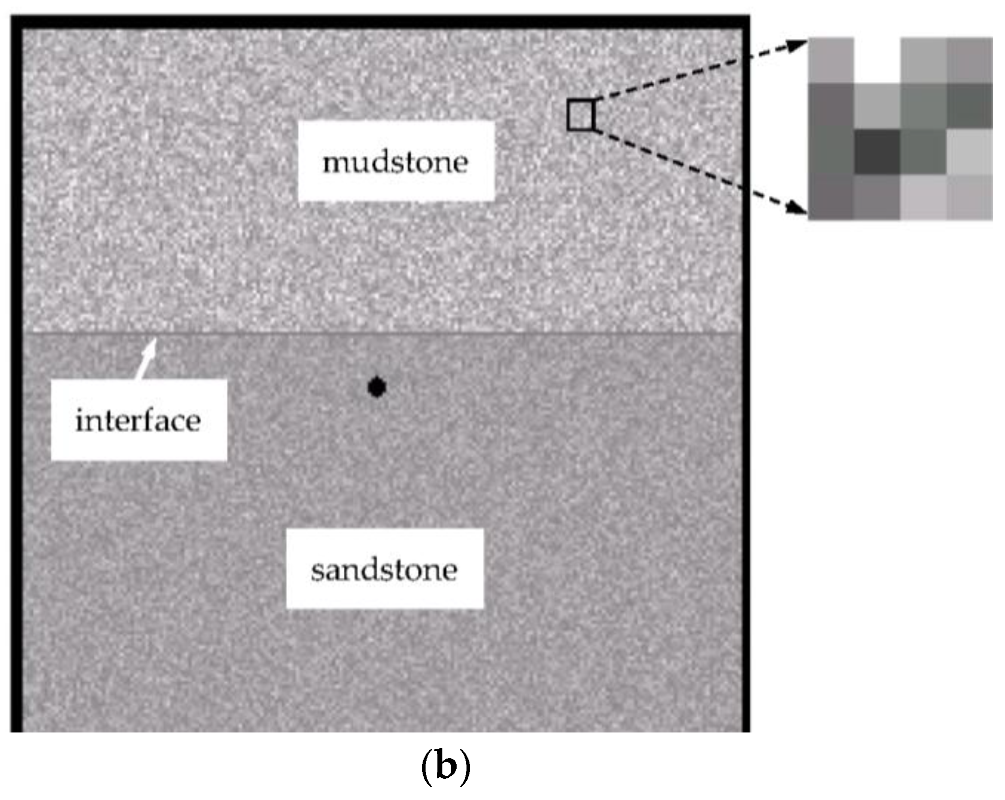
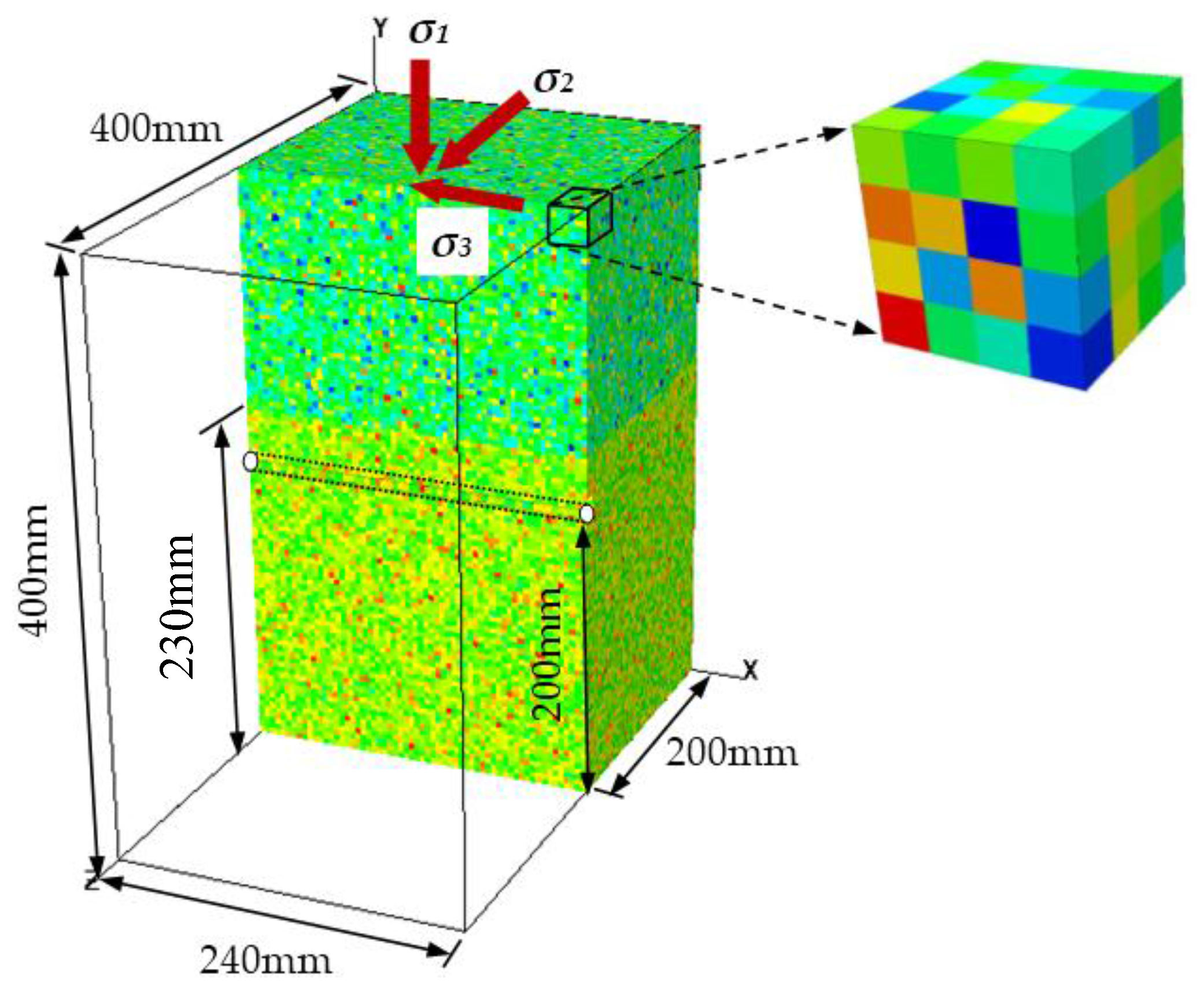
• The rock to be modelled is assumed to be composed of many mesoscopic elements. Here the mesoscopic elements that are used to represent the heterogeneity of rock are also utilized as the elements in the finite element analysis.
• The rock material at the elemental scale is assumed to be elasto-brittle with a residual strength. In the pre-peak region, the mesoscopic elements deform elastically, while in the post-peak region, the element will damage brittlely. The mechanical behaviour of rock is described by an elastic-damage constitutive law, and the residual strain/deformation upon unloading is not considered.
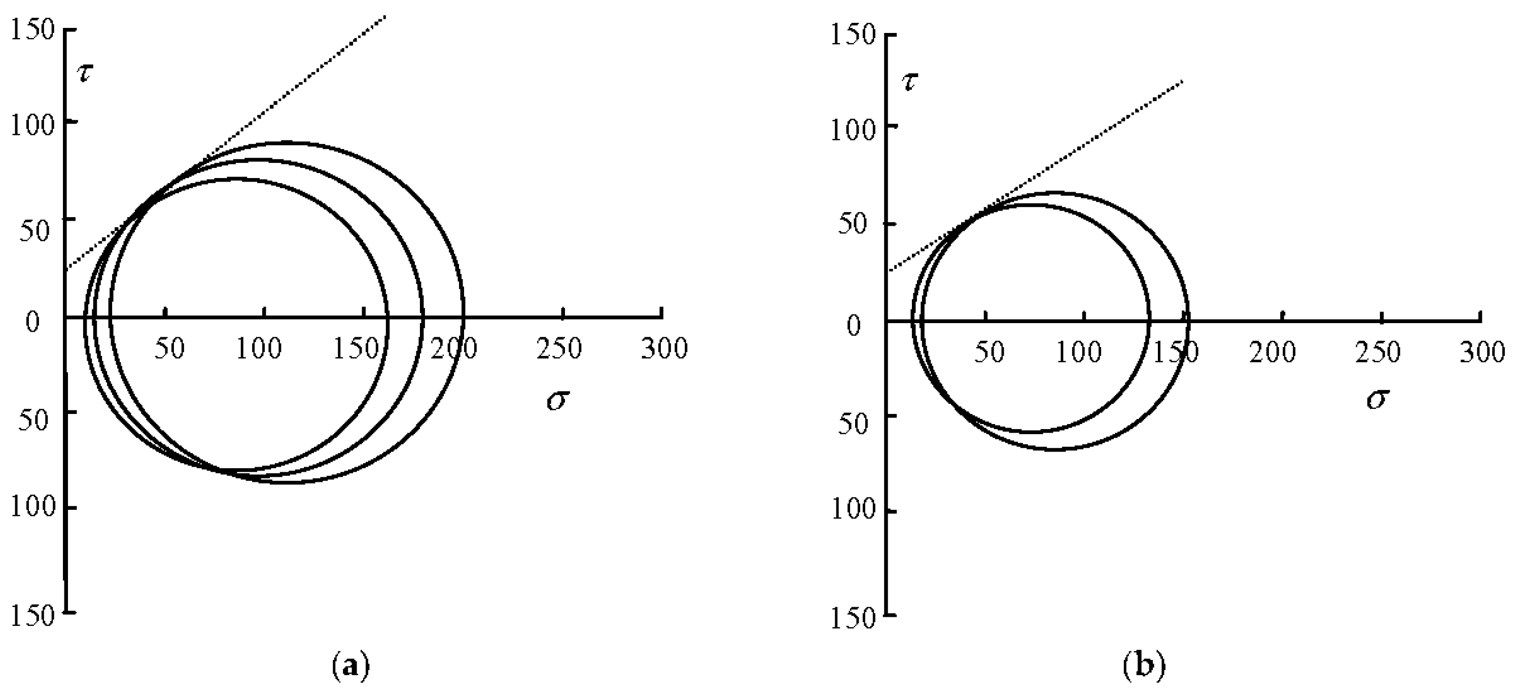
• An element is considered to fail in tensile mode when maximum tensile stress criterion is satisfied and fail in shear when the shear stress satisfies the Mohr-Coulomb failure criterion.
• The rock is assumed to be fully saturated with fluid flow governed by Darcy’s law. Additionally, the coupled process between stress/strain and fluid flow in the deforming rock mass is governed by Biot’s consolidation theory [22].
• The isotropic conditions are considered for the hydraulic behaviour at the elemental scale; the permeability of an element varies as a function of the stress state during elastic deformation, and increases dramatically when the element fails.
• The heterogeneity of rock materials is considered by assuming that the mechanical properties, such as Young’s modulus and the strength properties, conform to the Weibull distribution (specified by the Weibull distribution parameters).

Because of grain-scale heterogeneity, the failure strength in a rock can vary significantly. To include the statistical variability of the bulk failure strength in RFPA, the mechanical parameters of the model elements are assumed to follow a Weibull distribution [23]:

$$f\left(u\right)=\frac{m}{u_0}{\left(\frac{u}{u_0}\right)}^{m-1}\exp {\left(-\frac{u}{u_0}\right)}^m$$

(1)

where u is the element parameter (such as Young’s modulus, Poisson’s ratio, or strength properties), u₀ is the scale parameter related to the average value of the element parameter, and m is the heterogeneity index defining the shape of f(u) representing the degree of heterogeneity. A heterogeneous material can be numerically produced in a computer simulation by discretising with many elements, and each one is assumed to be isotropic and homogeneous. Systematic studies of the heterogeneity index m have been conducted previously [24,25].

The main governing equations in RFPA are as follows:

$$\text{Equilibrium equation:} \begin{array}{cc}{\mathsf{\sigma }}_{ij,j}=0& (i,j=1,2,3)\end{array}$$

(2)

$$\text{Geometrical equation:} \begin{array}{cc}{\mathsf{\epsilon }}_{ij}=\frac{1}{2}(U_{i,j}+U_{j,i})& {\mathsf{\epsilon }}_v={\mathsf{\epsilon }}_{11}+{\mathsf{\epsilon }}_{22}+{\mathsf{\epsilon }}_{33}\end{array}$$

(3)

$$\text{Constitutive equation:} {\mathsf{\sigma }}_{ij}^e={\mathsf{\sigma }}_{ij}-\mathsf{\alpha }p{\mathsf{\delta }}_{ij}=\mathsf{\lambda }{\mathsf{\delta }}_{ij}{\mathsf{\epsilon }}_v+2G{\mathsf{\epsilon }}_{ij}$$

(4)

$$\text{Fluid flow equation:} k{\nabla }^{2}p=\frac{1}{Q}\frac{\partial p}{\partial t}-\mathsf{\alpha }\frac{\partial \mathsf{\epsilon }v}{\partial t}$$

(5)

$$\text{Coupling equation:} k(\mathsf{\sigma },p)=\mathsf{\xi }{k}_0{e}^{-\mathsf{\beta }(\frac{{\mathsf{\sigma }}_{ii}}{3}-\mathsf{\alpha }p)}$$

(6)

where σ_ij is the total stress, ε_ij is the strain; U_i is the displacement; α is the coefficient of pore pressure, p is pore pressure, λ is the Lame coefficient, δ_ij is the Kronecher constant; G is the modulus of shear deformation, Q is Biot’s constant, k is the permeability; ξ (ξ ≥ 1.0) is a mutation coefficient of permeability to account for the increase in permeability once the element reach damage state, and β is the coupling parameter that reflects the influence of stress on the coefficient of permeability. Equation (6) is introduced to describe the dependency of the permeability on the stress and the damage. It has been determined experimentally that the coefficients α and ξ vary with the stress state and damage evolution of the rock. In this study, it is assumed that 0 ≤ α < 1 and ξ = 1 for the mesoscopic element in the elastic stage (indicated by D = 0, where D is the damage variable). Once damage occurs, the permeability of the mesoscopic element increases significantly. It is assumed that ξ = 5 for the damaged element (indicated by 0 < D < 1) and ξ = 100 for the full damaged element (indicated by D = 1) [20,26,27]. Correspondingly, α = 1 for the full damaged element.

In RFPA, continuum damage mechanics [28,29] is used to describe the constitutive law of the mesoscopic element. Initially, the element is considered to be elastic and its elastic properties can be defined by Young’s modulus and Poisson’s ratio. The stress-strain relationship of each element is considered to be linear elastic until the given damage threshold is attained. The sign convention used throughout this study is that compressive stresses and strains are positive. All following equations operate on effective stresses only.

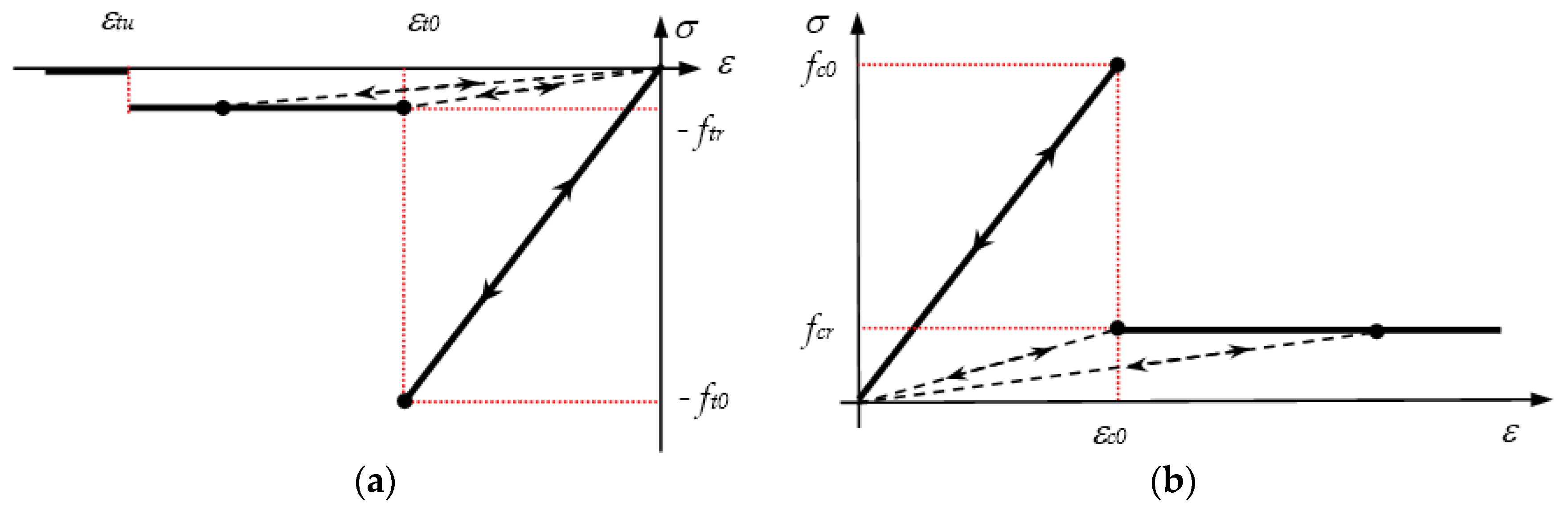
2.1. Damage Evolution of the Element in Tensional State

As illustrated in Figure 3a, the elastic damage constitutive relation for an element under condition of uniaxial tensile stress is used to govern the failure of an element. When the stress in an element satisfies the strength criterions, the element begins to accumulate damage and the elastic modulus of the element degrades gradually as damage progresses. The elastic modulus of the damaged element is defined as follows:

$$E=(1-D)E_0$$

(7)

where D represents the damage variable and E and E₀ are the elastic modulus of the damaged and undamaged elements, respectively. The element and its damage are assumed to be isotropic and elastic; therefore, E, E₀ and D are all scalar quantities.

When the tensile stress in the element reaches its tensile strength, $f_{t0}$:

$${\mathsf{\sigma }}_3\le -f_{t0}$$

(8)

the damage variable D of the element under uniaxial tension can be expressed as:

$$D=\{\begin{array}{cc}0& \epsilon >{\epsilon }_{t0}\\ 1-\frac{\mathsf{\lambda }{\mathsf{\epsilon }}_{t0}}{\mathsf{\epsilon }}& {\mathsf{\epsilon }}_{tu}<\mathsf{\epsilon }\le {\mathsf{\epsilon }}_{t0}\\ 1& \mathsf{\epsilon }\le {\mathsf{\epsilon }}_{tu}\end{array}$$

(9)

where λ is the residual tensile strength coefficient, which is given as f_tr = λf_t0. The parameter ε_t0 is the tensile strain at the elastic limit, which is called the threshold strain as shown in Figure 3a. ε_tu is the ultimate tensile strain of the element, describing the state at which the element would be completely damaged. The ultimate tensile strain is defined as ε_tu = η·ε_t0, where η is the ultimate strain coefficient.

In the current version of RFPA, it is assumed that the damage of an element under multiaxial stress is also isotropic. Following the method of extending a one-dimensional constitutive law under uniaxial tension to a complex stress condition, as proposed by Mazars and Pijaudier-Cabot [30], the constitutive equation described in Equation (9) then can be extended for application to three-dimensional stress states. Under multiaxial stress states, the element is assumed to be damaged in the tensile mode when the equivalent principal tensile strain $\overline{\mathsf{\epsilon }}$ [28] attains the threshold strain, ε_t0. The equivalent principal strain, $\overline{\mathsf{\epsilon }}$, is defined as follows:

$$\overline{\mathsf{\epsilon }}=-\sqrt{{\langle -{\mathsf{\epsilon }}_1\rangle }^2+{\langle -{\mathsf{\epsilon }}_2\rangle }^2+{\langle -{\mathsf{\epsilon }}_3\rangle }^2}$$

(10)

where ε₁, ε₂, and ε₃ are the three principal strains, and < > is a function defined as $<x>=\{\begin{array}{cc}x& x\ge 0\\ 0& x<0\end{array}$. The constitutive law for an element subjected to multiaxial stresses can be obtained by substituting the strain ε in Equation (9) with the equivalent strain $\overline{\mathsf{\epsilon }}$. The damage variable is then expressed as:

$$D=\{\begin{array}{cc}0& \overline{\mathsf{\epsilon }}>{\mathsf{\epsilon }}_{t0}\\ 1-\frac{\mathsf{\lambda }{\mathsf{\epsilon }}_{t0}}{\overline{\mathsf{\epsilon }}}& {\mathsf{\epsilon }}_{tu}<\overline{\mathsf{\epsilon }}\le {\mathsf{\epsilon }}_{t0}\\ 1& \overline{\mathsf{\epsilon }}\le {\mathsf{\epsilon }}_{tu}\end{array}$$

(11)

2.2. Damage Evolution of the Element in Compressive State

The constitutive law is given in Figure 3b when the element is under uniaxial compression and damaged in shear mode. To describe the element damage under a compressive or shear stress condition, the Mohr-Coulomb criterion is chosen as the second damage criterion:

$${\mathsf{\sigma }}_1-{\mathsf{\sigma }}_3\frac{1+\sin \mathsf{\phi }}{1-\sin \mathsf{\phi }}\ge f_{c0}$$

(12)

where ${\mathsf{\sigma }}_1$ and ${\mathsf{\sigma }}_3$ are the principal stresses, $\mathsf{\varphi }$ is the friction angle, and $f_{c0}$ is the uniaxial compressive strength. The damage variable under uniaxial compression is described as follows:

$$D=\{\begin{array}{cc}0& \mathsf{\epsilon }<{\mathsf{\epsilon }}_{c0}\\ 1-\frac{\mathsf{\lambda }{\mathsf{\epsilon }}_{c0}}{\mathsf{\epsilon }}& \mathsf{\epsilon }\ge {\mathsf{\epsilon }}_{c0}\end{array}$$

(13)

where ${\mathsf{\epsilon }}_{c0}$ is the compressive strain at the elastic limit, λ is the residual strength coefficient, and $f_{cr}/f_{c0}=f_{tr}/f_{t0}=\mathsf{\lambda }$ is assumed be true when the element is under uniaxial compression or tension.

When the element is in a multi-axial stress state and its strength satisfies the Mohr-Coulomb criterion, the maximum principal strain (maximum compressive principal strain) may be evaluated at the peak value of the maximum principal stress (maximum compressive principal stress), ${\mathsf{\epsilon }}_{c0}$.

$${\epsilon }_{c0}=\frac{1}{E_0}\left[f_{c0}+\frac{1+\sin \mathsf{\phi }}{1-\sin \mathsf{\phi }}{\mathsf{\sigma }}_3-\mathsf{\nu }\left({\mathsf{\sigma }}_1+{\mathsf{\sigma }}_2\right)\right]$$

(14)

where ν is Poisson’s ratio. In this respect, we assume that the shear damage evolution is only related to the maximum compressive principal strain, ε₁. Correspondingly, we substitute the maximum compressive principal strain ε₁ of the damaged element for the uniaxial compressive strain ε in Equation (13). Thus, Equation (13) can be straightforwardly extended to triaxial stress states for shear damage, as follows:

$$D=\{\begin{array}{cc}0& {\mathsf{\epsilon }}_1<{\mathsf{\epsilon }}_{c0}\\ 1-\frac{\mathsf{\lambda }{\mathsf{\epsilon }}_{c0}}{{\mathsf{\epsilon }}_1}& {\mathsf{\epsilon }}_1\ge {\mathsf{\epsilon }}_{c0}\end{array}$$

(15)

Based on the previous derivation of damage variable D and Equation (7), the damaged elastic modulus of an element at different stress levels can be calculated. In elastic stage, the unloaded element keeps its original elastic modulus and strength as those before strength threshold is attained. In damage stage, the unloaded element keeps its residual strength elastic and modulus. When unloaded, no residual deformation occurs in the model, i.e., the deformation can return to the original point along the stress path as shown in Figure 3. It should be emphasized that when D = 1, it can be calculated from Equation (7) that the damaged elastic modulus is 0, which would make the system of equations ill-posed; therefore, in the model a relatively small number, i.e., 1.0 × 10⁻⁵ MPa by default, is specified to the elastic modulus under this condition. Simultaneously, the Poisson’s ratio of the damaged element is assumed to be a larger constant (0.499 by default) and independent of the stress states.

Fracture initiation in geo-materials is considered to be either a tensile failure or shear failure in the material. However, what is the relationship of tensile crack and shear crack during the propagation process of hydraulic fractures? Field and experimental data show that most hydro-fractures are primarily tension fractures (particularly in brittle or hard rocks), because the tensile strength of rock is far lower than its compressive strength [12,18,31]. Moreover, extensive works have shown that even a crack which was, on a macroscopic scale, a shear crack, actually proceeded by an incremental process of aligned tension cracking [12,32,33,34]. In other words, the failure only becomes a ‘‘shear’’ zone once tensile fracture has progressed to the point where significant cohesion loss has occurred along the path of coalescing fractures and larger displacements become possible through kinematic feasibility. Therefore, it needs to be emphasized that an element cannot fail under a mixed mode and the damage of elements in tension is preferential to that in shear under all circumstances in RFPA. If the element is not damaged in tensile mode, the Mohr-Coulomb criterion is then used to determine whether the element is damaged in shear.

In the current version of RFPA, a “loose coupling” algorithm was used to simulate the coupled process between stress/strain and fluid flow (in loose coupling, two sets of equations are solved independently, but information/data is passed at designated time intervals in both directions between fluid flow and geomechanics). The solution steps of RFPA code are as follows:

(1)

initiate solution using a prescribed finite element mesh;

(2)

solve the fluid flow equation (Equations (5)) for the distribution of fluid pressure. The initial and boundary conditions, the spatial and time discretization, one can refer the published studies [20,35];

(3)

conduct an effective stress analysis to solve for the mechanical displacements (Equations (2)–(4));

(4)

based on the strength criterions (Equations (8) and (12)), check the element state (damage or elasticity), those elements that are stressed beyond the pre-defined strength threshold levels are assumed to be brittlely damaged;

(5)

reconcile the coupling between the stress and flow (where D = 0);

(6)

update the mechanical and hydraulic properties for the evolution of damage (where D > 0).

(7)

the model, with its associated new parameters, is then reanalysed. The next load increment is added only when there are no more elements strained beyond the strength-threshold corresponding to the equilibrium stress field and a compatible strain field. The model iterates to follow the evolution of failure along a stress path in pseudo-time, until the next time step.

Numerical modeling is an important tool for engineers to predict the geometry of fracture networks. However, the rigorous simulation of the real process of hydraulic fracturing is very challenging. Numerical models for hydraulic fracturing can roughly be classified into three kinds. The first kind is the models which need grid meshing in the whole region, such as the finite difference method, finite element method, extended finite element method and discrete element method, etc. The second kind is meshless methods. The third kind of fracture network simulation model is the models based on Displacement Discontinuity Method (DDM). Besides rigorous coupling model is needed (e.g., references [36,37,38]), any model intending to reproduce the real process of hydraulic fracturing should allow for the development of complex fractures. References [39,40] present very efficient methods for complex fracture as they do not require crack path continuity. The contributions [41,42] are efficient methods for discrete fracture with crack path continuity. Reference [43] proposed a framework for multiscale modeling of quasi-static crack growth. These methods for modeling arbitrary evolving cracks have potential applications in the modeling of hydraulic fracturing.

RFPA code employed in this study is using the continuum damage principle to simulate the crack propagation [44,45]. The fractured rock is assumed to be an equivalent continuous medium, and the crack corresponds to the damaged zone or flaw. Although the behaviours of the mesoscopic elements are governed by a simple constitutive law, the complex macroscopic behaviours, e.g., the fracturing process, can be represented by the interactions and coalescences of the damaged elements (with more and more isolated failure elements or cracks appearing, these elements or cracks may connect to each other to form the macroscopic fractures) [46]. Neither calculation of the stress intensity factor nor mesh rezoning is required in the model. One of the main features of this model is that there is no need for a pre-existing crack to simulate the crack initiation and propagation. This approach to simulate fracture is similar to a smeared crack model, i.e., the crack is smeared over the whole element and no special singular element is used for the finite element analysis of these mesoscopic elements, which greatly simplifies the simulation of crack initiation, propagation and coalescence. The advantage is to leave the mesh topology untouched [34,47,48]. In recent years, with the advancing in the performance of computers, an increasing number of researchers have tried to use the similar principle to model rock/concrete damage behaviours [48,49,50,51]. Based on the strength criterions (Equations (8) and (12)), if those elements that are stressed beyond the pre-defined strength threshold levels are assumed to be irreversibly damaged, the stiffness and strength of the damaged elements are reduced, permeability is increased accordingly. The elements whose ultimate tensile stress has been attained are displayed as cracks with black colour in the post-processing figures.

3. Numerical Simulation and Discussion

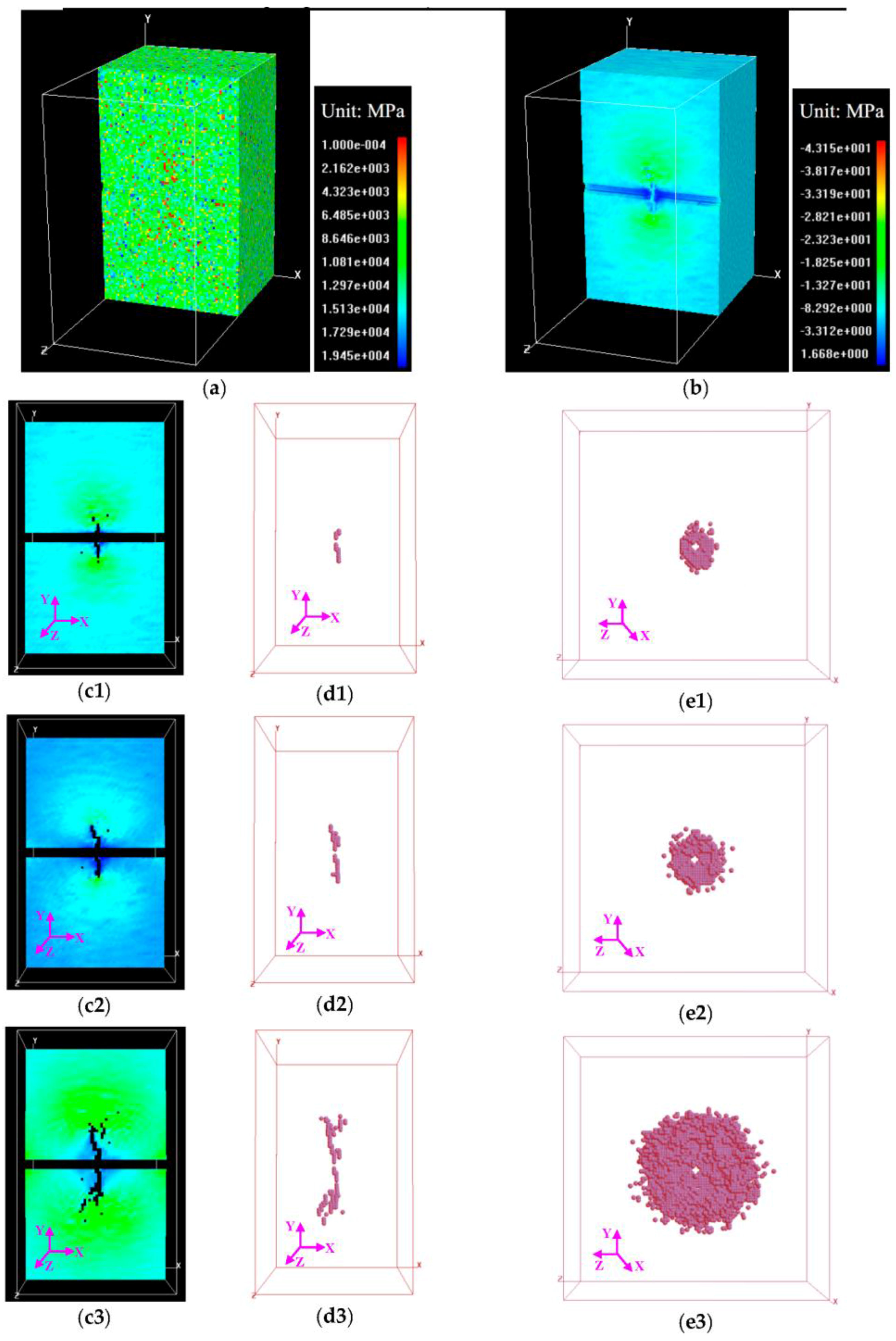
3.1. Hydraulic Fracturing Process in the Models without Interfaces

First, a small-scale model as shown in Figure 4 is used to investigate the behaviour of the fracturing away from a horizontal wellbore. In this model, a horizontal wellbore with a diameter of 24 mm is assumed to be located at the centre of a 400 mm × 400 mm × 240 mm block. The block was discretised into 600,000 elements. A perforated section (which is subjected to hydraulic pressure) is located in the centre of the wellbore. In this study, the propagation of hydraulic fracture is assumed to be driven by an incompressible and Newtonian fluid (water). An increasing pressure is applied along the boundary of the interior hole in the perforated section to simulate the pressurised fluid. The rate of pressurisation increase is kept constant throughout the numerical tests at 0.05 MPa per loading step. A constant pressure condition (p = 0 MPa) is imposed on the outward boundaries of the block. As the model is not a field case but a demonstration case with a relatively small geometry, the body stresses resulted from weight is not considered and problem will be solved quasi-statically, i.e., the fluid flow is simulated as a steady process.

Five different cases are simulated to illustrate the influence of the far-field stress on the hydraulic fracturing behaviour. The applied confining stresses, representing the effect of the far-field stresses, are reported in

Table 1. Confining stresses for five cases.

Confining stress	Case I	Case II	Case III	Case IV	Case V
${\mathsf{\sigma }}_1$ (MPa)	20.0	20.0	20.0	20.0	20.0
${\mathsf{\sigma }}_2$ (MPa)	8.0	10.0	13.0	15.0	18.0
${\mathsf{\sigma }}_3$ (MPa)	5.0	5.0	5.0	5.0	5.0

(note that compressive stress is defined to be positive in this study), and the wellbore axis is aligned with the direction of σ₃.

Because this study is motivated by the practical engineering of hydraulic fracturing of beach-bar sandstone reservoirs in Shengli Oilfield, the material properties are chosen based on the laboratory experiment data of the rock core from one of the beach-bar sandstone reservoirs [4].

Table 2. The mechanical properties of rock cores from one of the beach-bar sandstone reservoirs in Shengli Oilfield [4].

Well No.	Rock Formations	No. of Rock Core	Confining Stress (MPa)	Peak Strength (MPa)	Elastic Modulus (GPa)	Poisson’s Ratio
Bin-438A	mudstone	0-1	10	160.53	19.56	0.162
		0-2	15	179.36	21.58	0.174
		0-3	20	197.65	26.72	0.204
	sandstone	90-1	15	140.77	11.08	0.236
		90-2	20	154.20	11.53	0.287

contains the experiment data of mechanical properties and Figure 5 shows the corresponding Mohr-Coulomb envelopes of the sandstone and mudstone from the beach-bar sandstone reservoir. Based on Table 2 and Figure 5, it is found that the strength and stiffness of mudstone are generally higher than those of sandstone, while the Poisson’s ratio of mudstone is generally lower than that of sandstone. Although the mechanical properties listed in Table 2 are taken from triaxial experiments, these data have reference value for uniaxial parameters that are needed in numerical modelling in this study. The mechanical parameters used in the modelling are reported in

Table 3. Physico-mechanical parameters employed in simulations.

Parameters and Unit	Sandstone	Mudstone
Heterogeneity index (m)	2.5	2.5
Young’s modulus (E0), GPa	9	15
Uniaxial compressive strength ($f_{c0}$), MPa	100	120
Poisson’s ratio (v)	0.25	0.2
Internal friction angle ($\mathsf{\varphi }$), °	30	35
Uniaxial tensional strength ($f_{t0}$), MPa	10	12
Permeability coefficient (k0), cm/s	1.0 × 10−7	1.0 × 10−8
Coefficient of the pore water pressure (unfractured) (α)	0.0001	0.0001
Coefficient of the pore water pressure (fractured) (α)	1.0	1.0
Coupling coefficient (β)	0.01	0.01

. In Table 3, the Young’s modulus, uniaxial compressive strength, and Poisson’s ratio of mudstone and sandstone are derived from Table 2 and Figure 5. Permeability is from reference [4]. Coefficient of the pore water pressure and coupling coefficient are from references [20,27,44]. As the tensile strength of rock is much lower than its compressive strength, the compressive/tensile strength ratio is selected to be 10, which is within the range of experimental values for rock [45,46].

Using RFPA, a parallel FEM computation on high-performance computer (HPC) cluster is performed. As the first type case, the model is assumed to contain single stratum, i.e., the model is only composed of sandstone. Figure 6 shows the evolution of stress and fracture profile during the hydraulic fracturing process for Case III. One can find that the propagation of the hydraulic fractures is controlled by the far-field stress orientation. The hydraulic fracture selects the path of least resistance through the material, and the random locations of the individual heterogeneities result in an irregular hydro-fracture trajectory.

The pressures for fracture initiation for the five cases are presented in Figure 7. The analytical results based on Equation (16) are also plotted in Figure 7. The hydraulic fracturing criterion [52,53] is among the mostly widely used constructs in hydraulic fracturing theory. Hubbert and Willis [52] argued that a tensile fracture initiates when the effective tangential stress at the wellbore wall reaches the tensile strength of the rock. The borehole fluid breakdown pressure, $P_b$, is given by:

$$P_b-p_0=3{\mathsf{\sigma }}_{\min }-{\mathsf{\sigma }}_{\max }+f_t-2p_0$$

(16)

where ${\mathsf{\sigma }}_{\min }$ and ${\mathsf{\sigma }}_{\max }$ are the lowest and highest principal stresses in the plane perpendicular to well, respectively, $p_0$ is the initial fluid pore pressure and $f_t$ is the tensile strength of impermeable rock.

It is shown that the distribution of the breakdown pressure in the numerical simulations is generally consistent with the analytical results, although the match between numerical and analytical deteriorates with increasing deviatoric stress. In the traditional theory of hydraulic fracturing, the rock formation is assumed to be homogeneous and the fracture is smooth, and the breakdown pressure, P_b, is then given by the peak pressure when the hydraulic pressure is increasing, indicating the initiation of hydraulic fracturing. However, in reality, a perfect fracture (i.e., a perfectly planar fracture perpendicular to any stress direction) is not possible in the highly heterogeneous reservoir rock formation. For example, although the fractures initiated in a plane, they branched out after growing for a short distance. As soon as the fracture propagates slightly out of plane, the shear stress component reorients the fracture towards the preferred direction for fracture propagation with minimum resistance. Isolated fractures generated from weak elements also open within the rock mass. The observation that hydraulic fractures developing with offsets in their path require high fluid pressures to sustain fracture growth has been suggested by Medlin and Fitch [54]. Based on numerical studies of small-scale models, Zhang et al. [15] and Hossain and Rahman [55] also demonstrated that the complex fracture growth in field may lead to the requirement of a higher treatment pressure. Our study has established that the fracture develops a complex geometry through repeated deflections and branchings during propagation. This phenomenon is expected to result in flow constriction and a higher treatment pressure. Meanwhile the deviatoric confining stress plays an important role in the fracture propagation. For example, in the case with lower deviatoric confining stress (e.g., 2.0 MPa), the hydraulic fracture can deterministically select in part the path of least resistance through the rock matrix based on its statistical features, and the random locations of the local heterogeneities. However, in the cases with higher deviatoric confining stresses (e.g., 12.0 MPa), the fractures “have to” strictly propagate along the orientation of the maximum principal stress, encountering, branching and/or bypassing some grains with higher strength and stiffness, which indicates that a higher pressure is required for the fractures to continue initiating and propagating.

To investigate the effect of the rock strata properties on the fracturing mode, another two cases (Cases VI and VII) were considered. In Case VI, the model contains two rock strata, i.e., sandstone (the bottom layer) and mudstone (the top layer), while in Case VII, the strength properties of mudstone layer are assumed to be increased by 50%, compared with those of Case VI. The boundary and other parameters were kept constant in Case VI. Figure 8 shows the corresponding numerical results for Cases VI and VII.

In Case VI, the mechanical properties are kept constant at the particular values listed in Table 3. The fracture from the sandstone layer can extend to the mudstone layer, while in Case VII, the initiation and propagation of fractures are generally restricted within the sandstone layer. For cases with perfectly bonded interfaces, the elastic solutions for a crossing fracture can be found in the work by Erdogan and Biricikoglu [56]. It is shown that the difference in the mechanical properties of adjacent rock layers can influence the hydraulic fracturing process in the cases without interface (or the adjacent rock layers are perfectly bonded by a perfect interface). Compared with Cases III and VI, stronger adjacent rock layers with higher toughness are found to efficiently resist fracture propagation from the bottom layer.

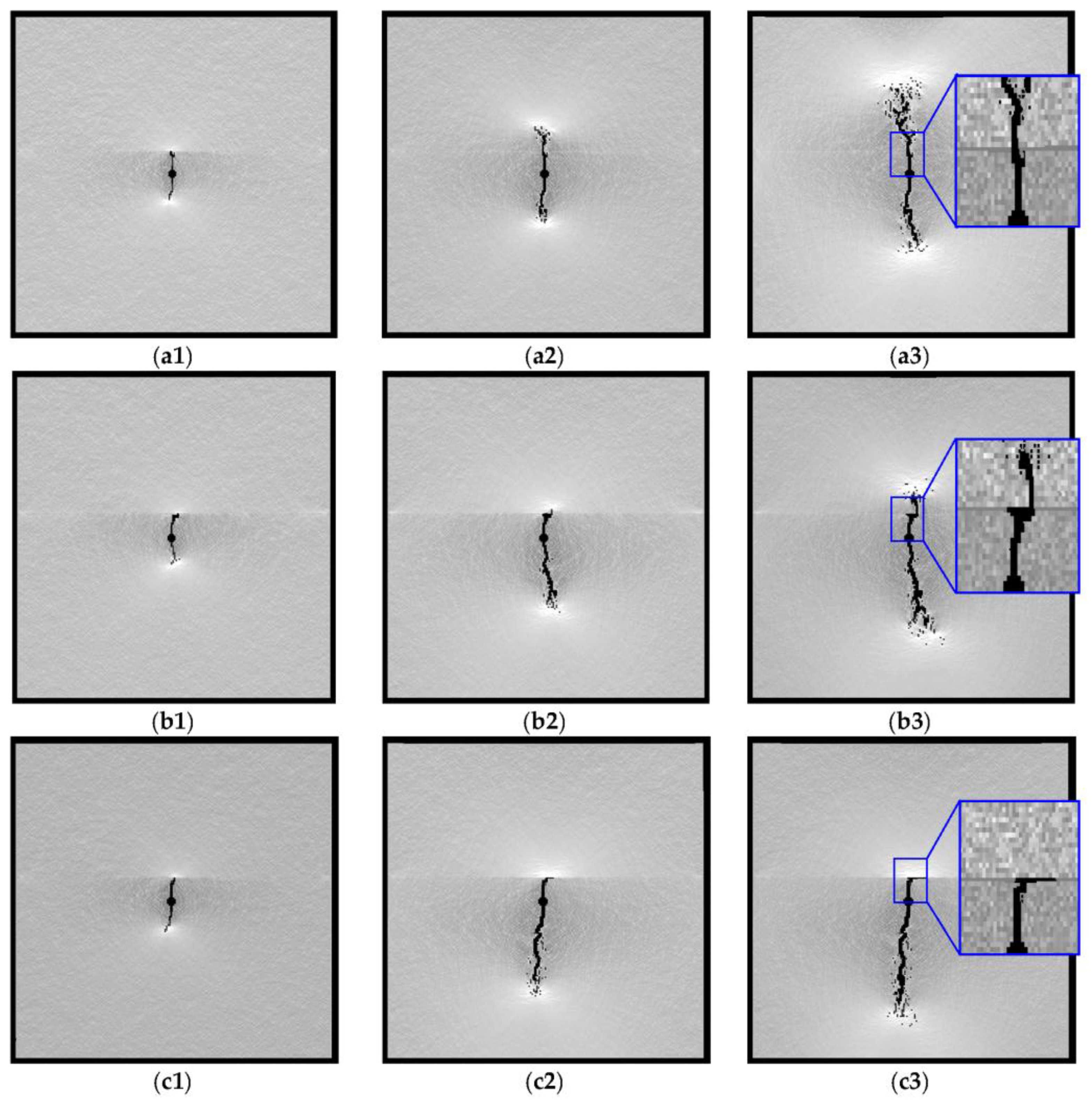
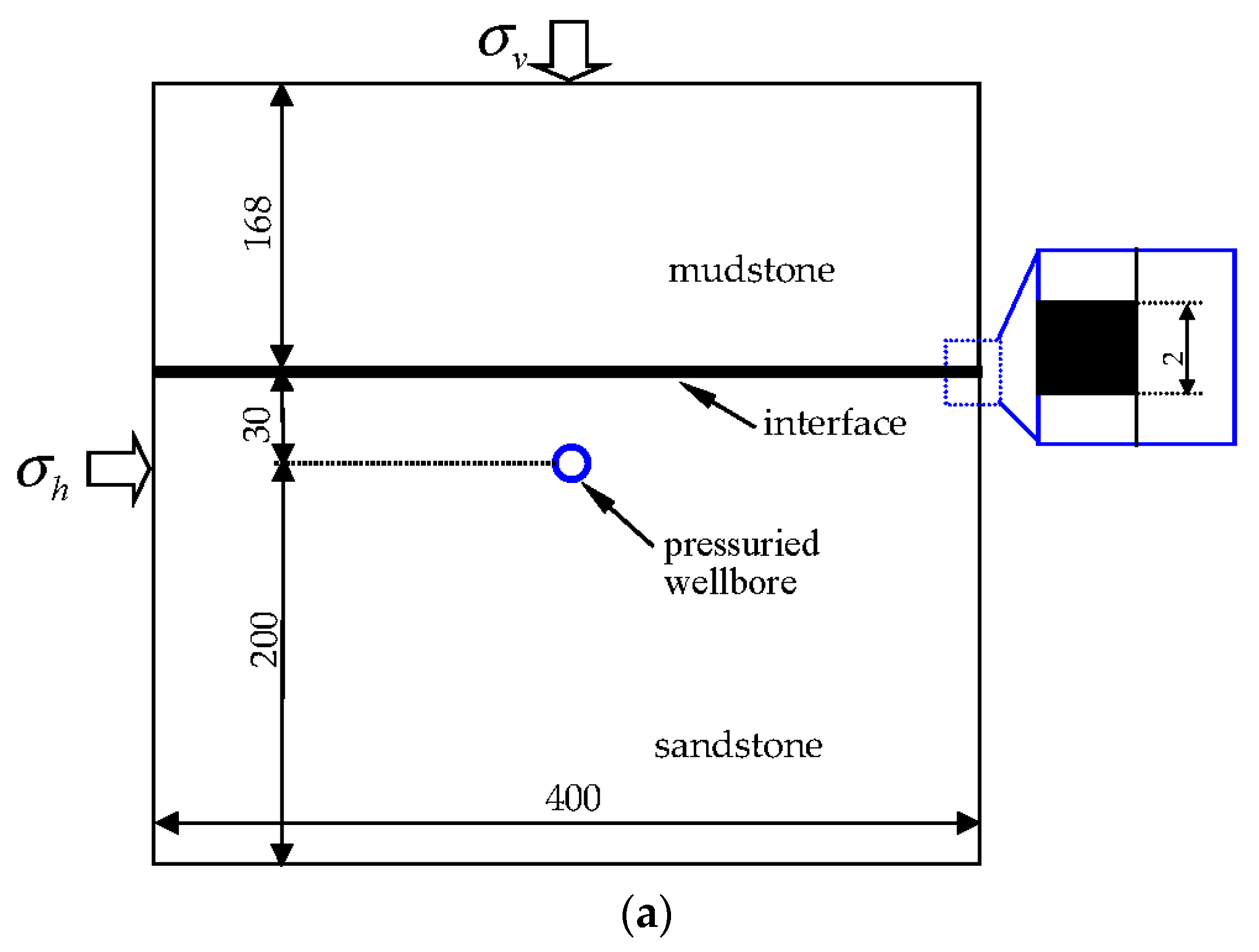
3.2. Hydraulic Fracturing Process in the Models with Interfaces

In the numerical studies above, the interface surfaces between the sandstone and mudstone layer are assumed to be strong enough to prevent any other fracture initiation on the interface, i.e., the top and bottom rock layers are perfectly bonded. However, the assumption of perfectly bonded interfaces is often incorrect for geological interfaces, since most interfaces have limited strength. As a fracture propagates toward an interface, tensile stresses develop across the interface. Debonding and subsequent opening of the interface may occur when the interface normal tensile stresses exceed the prescribed interface tensile strength. Geological discontinuities such as natural joints, faults and flaws, as well as bedding planes, in reservoir rocks and in ore bodies may contribute to the deflections and branching of hydraulic fractures [5,7,57]. In this section, we attempt to highlight the fracturing process developed in layered rocks, and to use these concepts for a better understanding of the demonstration models established from the field observations in beach-bar sandstone reservoirs in Shengli Oilfield. Basically, there are three points that are crucial in fracturing across interfaces: (1) confining stresses, representing the effect of the in-situ stresses; (2) strength of the interfaces; and (3) material properties of the layers on either side of the interface.

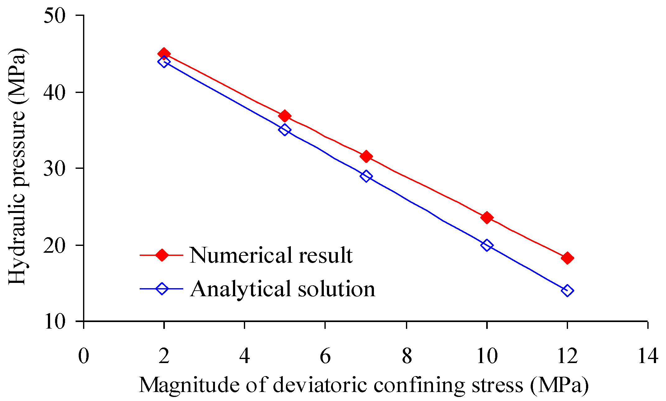
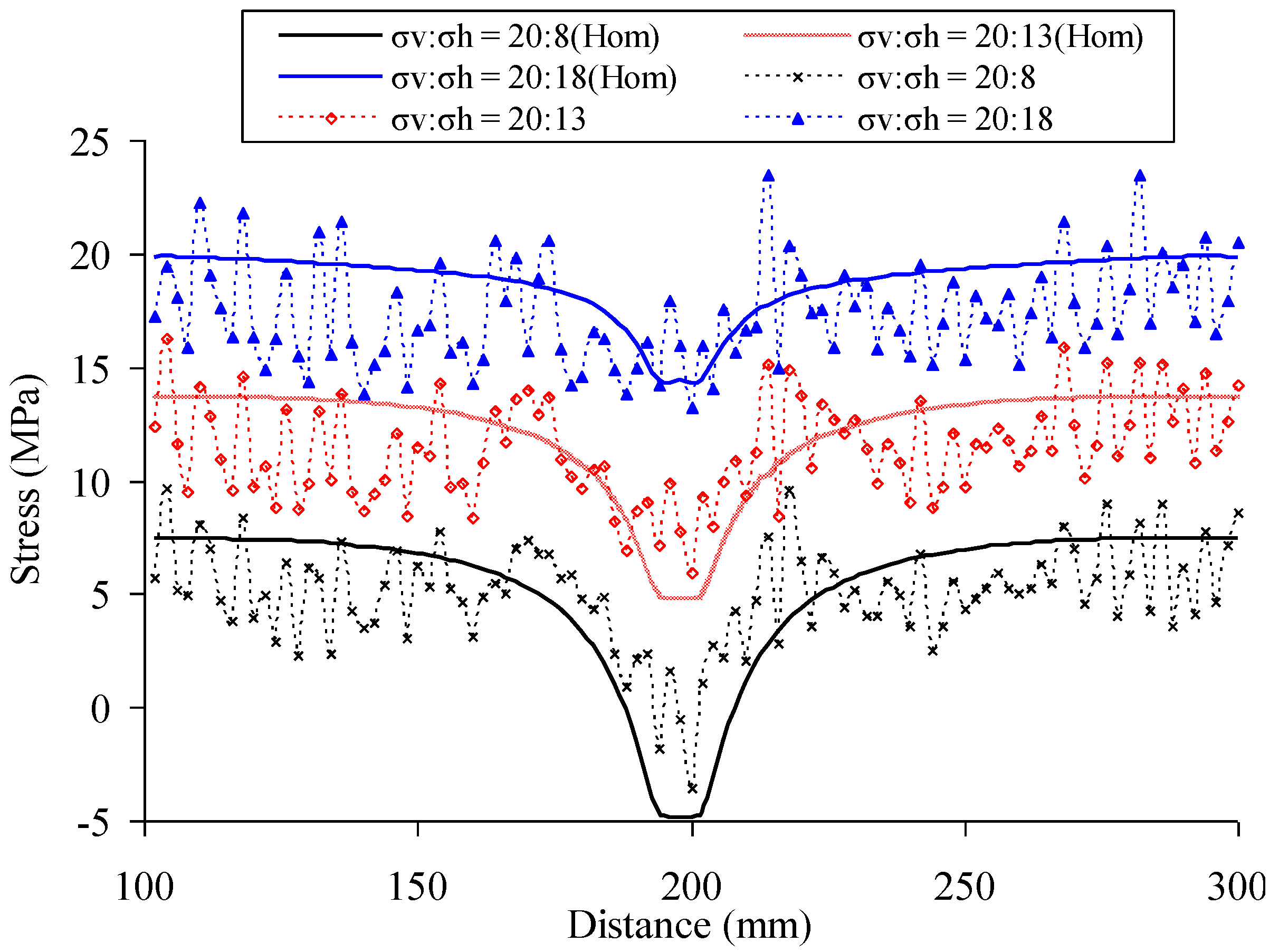
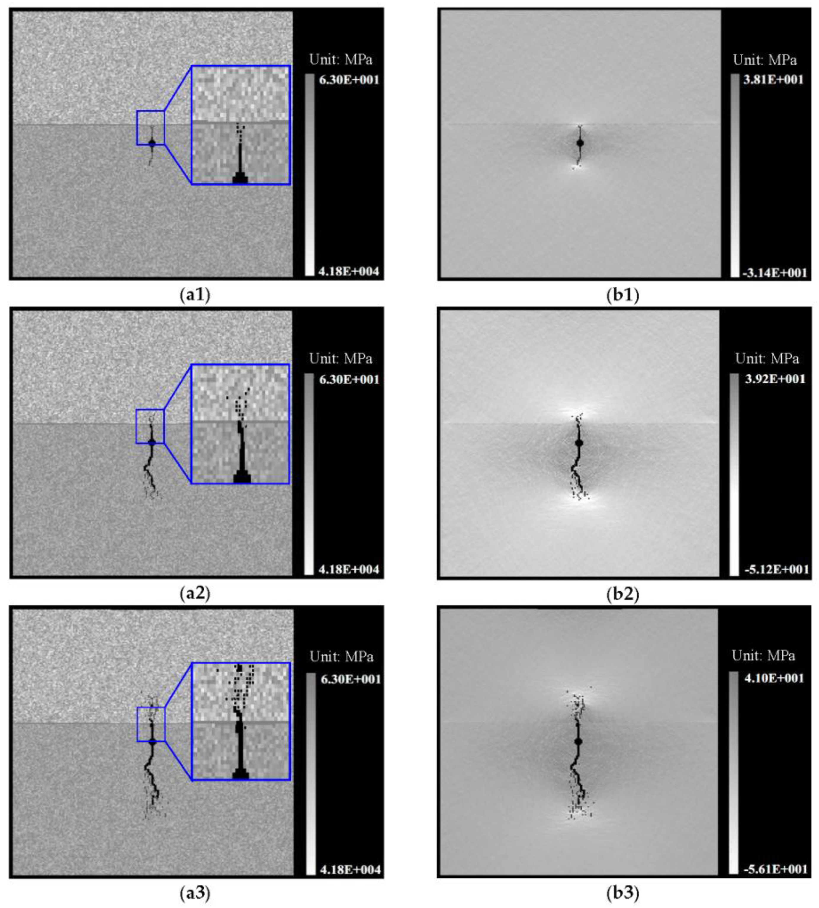
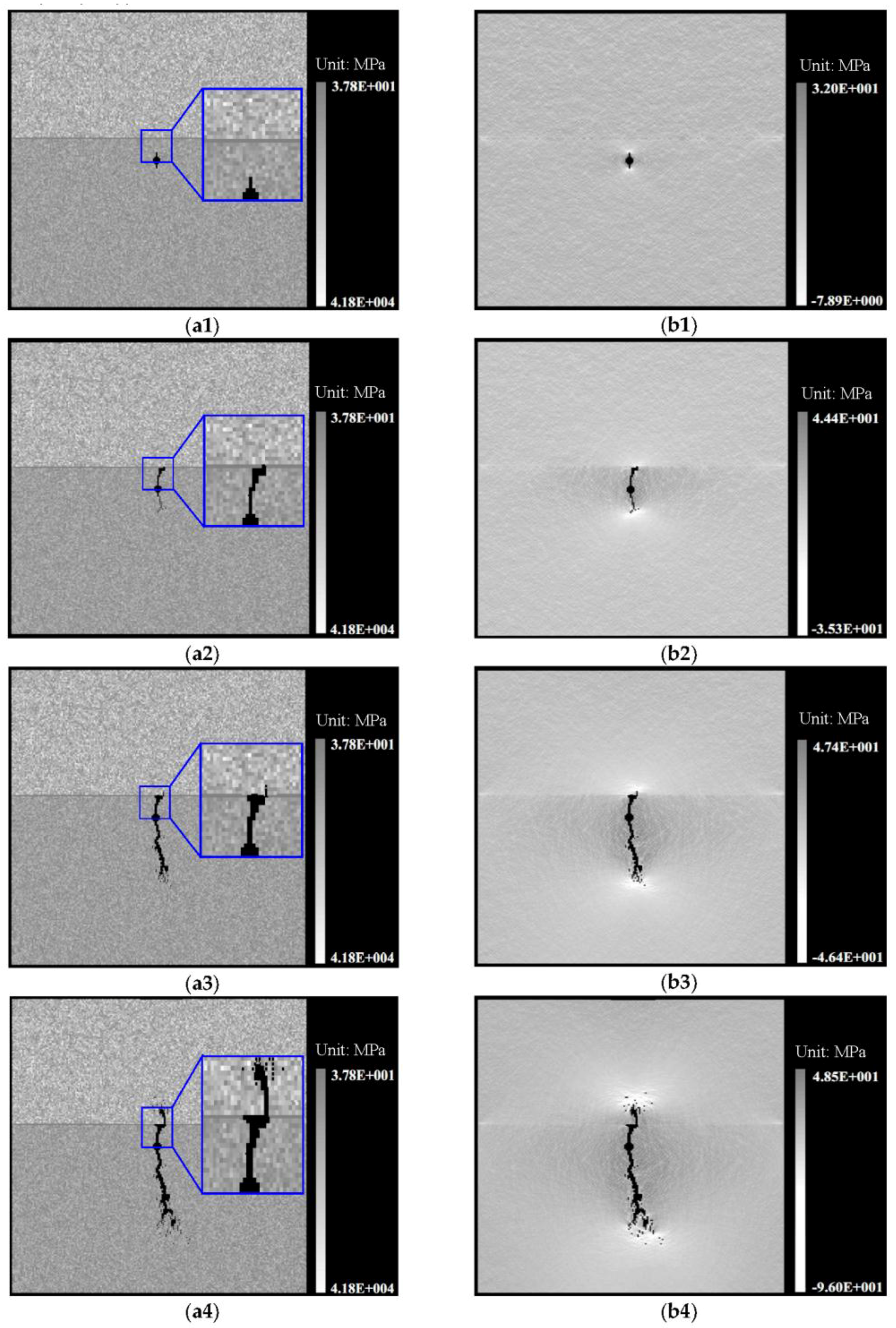
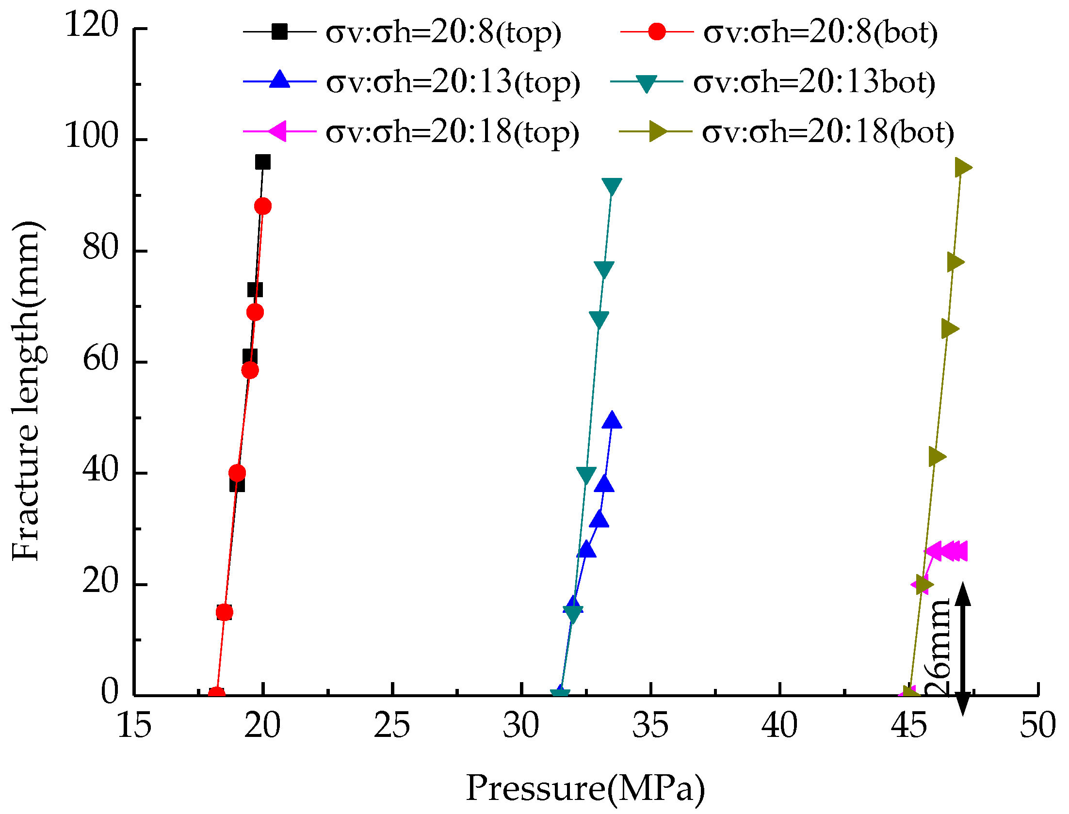
3.2.1. The Influence of Confining Stress on Hydro-Fracture Propagation

The success or failure of hydraulic fracturing technology is largely dependent on the design of fracture configurations and the optimisation of treatments compatible with the in-situ conditions of a given reservoir. To make a detailed investigation on the influence of in-situ stresses on hydraulic fracture propagation in a model with a bedding plane (referred to as an interface), a 2D numerical model, as shown in Figure 9, is first employed.

The model has geometry of 400 mm × 400 mm, and has been discretised into a 40,000 element mesh. The bottom layer, hosting the hydro-fracture, is sandstone, while the top layer is mudstone. Totally three cases are simulated to illustrate the influence of the far-field stresses on the hydraulic fracturing behaviour. The applied constant confining stresses, which represent the effect of the far-field stresses, are listed in

Table 4. Confining stresses in the cases with an interface.

Case	${\mathsf{\sigma }}_{\mathit{v}}$ (MPa)	${\mathsf{\sigma }}_{\mathit{h}}$ (MPa)
I	20.0	8.0
II	20.0	13.0
III	20.0	18.0

.

The mechanical parameters for the three cases are kept constant at the values listed in Table 3. The hydraulic pressure applied along the boundary of the wellbore is an increasing fluid pressure with an increment of 0.05 MPa per loading step. The diameter of the wellbore is 8 mm. In this model, an interface is embedded between the sandstone and mudstone. In RFPA, a specified type of material is then used to represent the interface between different rock matrixes [58,59].

The interface is assumed to consist of ‘‘weak material’’ with a lower strength and stiffness compared to the sandstone and mudstone. Because it’s hard to evaluate the accurate strength data for interfaces in beach-bar sandstone reservoirs, an interface is simulated with mechanical properties of E = 500 MPa, v = 0.4, c = 3.0 MPa, and f_t = 1.0 MPa, referring to the previous studies [60,61]. In this model, the interface is referred to as the moderate-strength interface.

Abrupt changes in mechanical properties between horizontal layers can also significantly affect the opening up of discontinuities ahead of a propagating hydrofracture. For example, a layer with a low Young’s modulus (a soft layer) tends to suppress, whereas a layer with high modulus (a stiff layer) tends to magnify, the tensile stresses around the hydrofracture tip [11,62]. Before reporting the results of the simulations in progressive fracture, the stress distribution that governs the model’s behaviour was first focused on. Figure 10a shows the fluid pressure distribution when the applied pressure in the wellbore is 25.0 MPa. One of the most widely used techniques to visualize stress fields is the technique of photoelasticity. The numerical photoelasticity in Figure 10b provides the contours of difference in principal stresses. Because the stresses adjacent to interface are the main concern, we just show a small portion of the model in a big box. The fringes in general appear as broad bands, the thickness of the fringe is indicative of the gradient of the stress variable. The fringes are very broad when the gradient is small, and vice versa. The zone of high density of fringes indicates a zone of stress concentration. It is shown that the interface acts as a barrier for the stress to transfer, which induces evident stress concentration within the region adjacent to the fracture tip and interface. However, in reality, the rock formation in the field is usually heterogeneous. In order to demonstrate the difference in stress fields between models with and without considering the rock heterogeneity, the numerical photoelasticity for the heterogeneous case is further presented in Figure 10c. These two computed fringe patterns clearly show that the heterogeneity has a strong influence on the stress fields in the model. Since it is not possible to obtain the fringe patterns in heterogeneous materials, the numerical results are of significance to improve our understanding of the stress field in such a layered and heterogeneous model.

For a quantitative evaluation of the heterogeneity and in-situ stress effect, we have shown in Figure 11 the minimum principal stress along the top of the interface (the mudstone side of the interface). In Figure 11, the smooth curves are the results for the homogeneous cases, while the fluctuant ones are the results for heterogeneous cases. It is shown that the changes in confining stress configuration between horizontal and vertical stress can significantly affect the opening up of discontinuities ahead of a propagating hydro-fracture. Under conditions of higher deviatoric confining stress, a more evident high tensile stress becomes concentrated near the region of interface so that it would normally be easy for the hydro-fracture tip to enter, and propagate through the top layer. Again, the influences of material heterogeneity on the stress distribution are illustrated very clearly. We find that the maximum fluctuations of minimum principal stress are 50% of the mean stress for this heterogeneous case. It is obvious that ignoring these stress fluctuations may result in wrong conclusions if fracturing process is conducted.

To clearly show the hydraulic fracturing process, the case with σ_v = 20.0 MPa and σ_h = 13.0 MPa (i.e., the deviatoric confining stress is 7 MPa) is focused on. Figure 12a illustrates the development and formation of the hydraulic fractures in detail, with the relative magnitude of the elastic modulus of the mesoscopic elements indicated by the grey scale. A brighter shade of grey corresponds to a higher Young’s modulus. In Figure 12, the dark elements represent the nucleated flaw. Fractures form through the connection of flaws. Figure 12b shows the evolution of the fracture and stress field (the minimum principal stress) during the hydraulic fracturing process. The grey scale indicates the relative magnitude of the stress within the elements. The elements with lighter shade of grey have relatively higher stresses. As the hydraulic pressure increases, the average maximum tensile stress increases along the boundary of the wellbore and fracture, particularly fracture tips display remarkable stress concentrations.

The hydraulic fracture deterministically selects the path of least resistance through the material based on its statistical features, and the random locations of the local heterogeneities result in an irregular hydraulic fracture trajectory. As shown in Figure 12, the fracturing paths on the top and bottom sides of the wellbore are different from one another. On the top side, as the fracture propagating, the fracture “senses” the interface before coming in contact with it. The interface material provides stress transfer fluctuation between the sandstone and mudstone. Before the fracture approaches the interface, there is a large area of stress concentration between the fracture tip and the interface.

As the fracture approaches and penetrates the interface, a maximum tensional stress is observed in mudstone layer. However, the fracture does not grow at this location and fully penetrate through the interface (Figure 12(a2)). Instead, the fracture is blunted and propagates near the interface, because the strength of the mudstone layer is relatively strong and the fracture needs more energy to keep propagating forward. After the accumulated fluid pressure is reached to a certain level, an offset fracture is initiated from the blunted fracture (Figure 12(a3)). Once the fracture resumes its forward propagation, the stress concentration near the interface begins to decrease and the stress concentration is transferred to the fracture tip. Once the fracture passes the interface, it continues to propagate within the mudstone along the orientation of the maximum principal stress. On the bottom side of the wellbore, the fracture keeps propagating forward with the increasing fluid pressure, although the fracture path is flexural (rather than straight).

The simulations in this study account for any previously failed neighbouring elements. Following the first redistribution of stress, additional elements may fail owing to the stress increment. Therefore, in each loading step, the stress redistribution procedure is repeated until all of the elements for which the strength criteria are met and are stress-free, the released stresses are distributed between the intact neighbours, and global equilibrium of the sample is achieved. The next loading step is then performed. The broken elements form clusters that grow and coalesce as the load increases. Finally, the macroscopic failure zone, i.e., a fracture, is formed with the mutual connection of a plurality of such clusters. The final result of the micro-damage accumulation is a brittle fracture initiation and propagation rather than a single event.

The variation of the fracture pattern is highly sensitive to the interaction between the isolated fractures and the local disorder features of the rock matrix in the highly stressed field. In practice, the rock formation in field is usually heterogeneous. As a result, the fracture path is rough, and mixed-mode fracture propagation further affects the non-planar fracture growth in the non-preferred direction. In reality, there are two types of failure, high-stress failure and low-strength failure, for different materials. In a homogeneous material, failure begins at the high-stress site, whereas in a heterogeneous material (e.g., rock), failure may start at the weaker locations because of the presence of pores, microfractures, and grain boundaries. This observation led Fairhurst [63] to introduce the notion of ‘‘stress severity’’, which represents the ratio of the theoretical stress at the moment of failure to the stress that would theoretically be necessary for failure at any given point. Therefore, maximum tension stress is not the only consideration for fracture initiation. Fractures typically initiate at local concentrations of tensile stress around flaws, such as fossils [57]. Since flaws produce greater stress concentrations, the location of fracture initiation depends on the distribution of the flaws as well as the magnitude of maximum principal tension stress [64].

Figure 13 is the numerical results for the case with a higher deviatoric confining stress (σ_v:σ_h = 20:8). It is shown that the fracture penetrates straight through the interface and keeps propagating in the mudstone layer. While for the case with a lower deviatoric confining stress (σ_v:σ_h = 20:18) (Figure 14), the fracture is fully blunted and stops at the interface. Finally a T-shaped fracturing mode is formed.

It is clear that the large difference between the vertical and the horizontal in situ stresses, can give rise to higher interaction stresses and more difficulty for fracture propagation along the interface. Fracture termination is more likely under conditions of lower deviatoric confining stress. A larger vertical stress can suppress the small and localized interface opening that acts to terminate fractures and promote either step-over fractures or fracture propagation through interfaces. The trend of fracture growth from numerical result here is consistent with the experimental results that increased interface normal compression can encourage fracture propagation through the interface [65,66].

Figure 15 shows the variation of fracture length in vertical direction with the increasing hydraulic pressure. For the case with a higher deviatoric confining stress, the fractures on the top and bottom sides of the wellbore are generally symmetric. While for the other two cases, the growth of the top and bottom fractures is evidently asymmetric, particularly for the case with a lower deviatoric confining stress. Once branches and offsets appear during the hydraulic fracturing process, the fractures that develop such offsets in their path require higher fluid pressure to sustain fracture growth, as was suggested by previous studies [15,54,55]. In the practical engineering of hydraulic fracturing of beach-bar sandstone reservoirs in Shengli Oilfield, unusual high pressures are often recorded [67,68]. The peak values of the pressure recorded in beach-bar sandstone reservoirs in Shengli Oilfield is 20%–30% higher than that recorded in conventional reservoirs [4]. Numerical results show that the fracturing behavior of branches and offsets between the sandstone and mudstone layers is one of the sources of high treating pressures and reduced fracture volume.

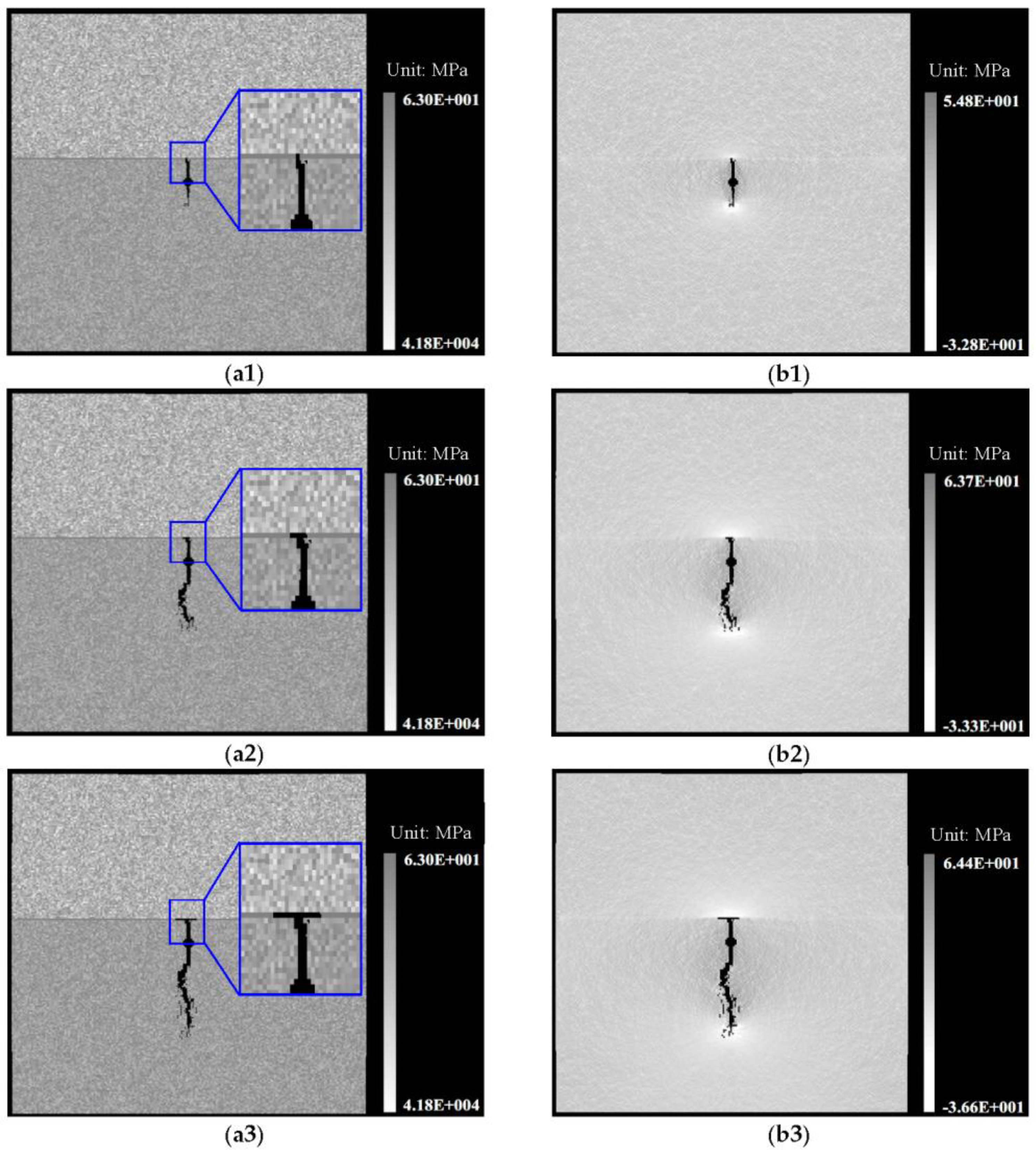
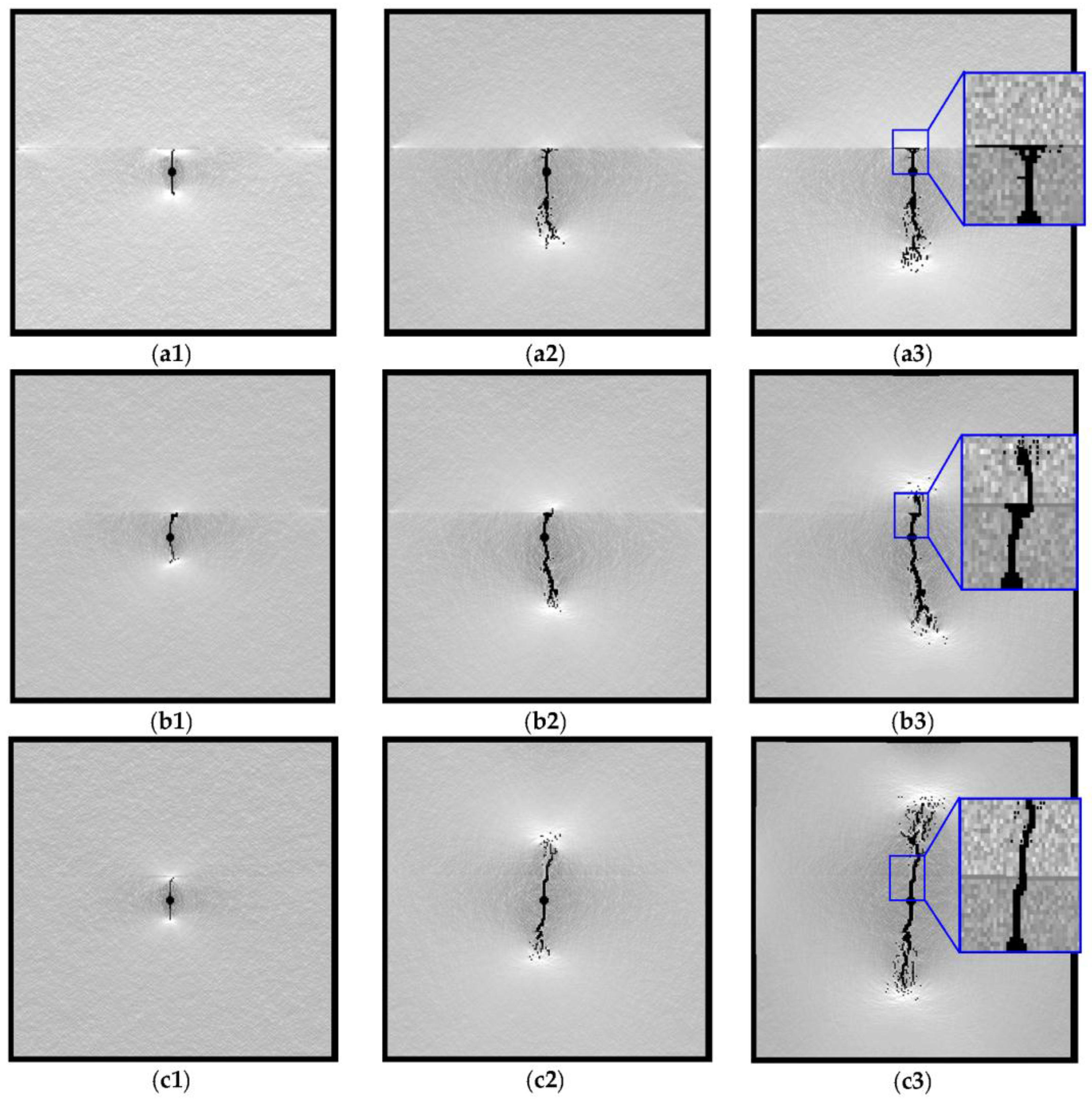
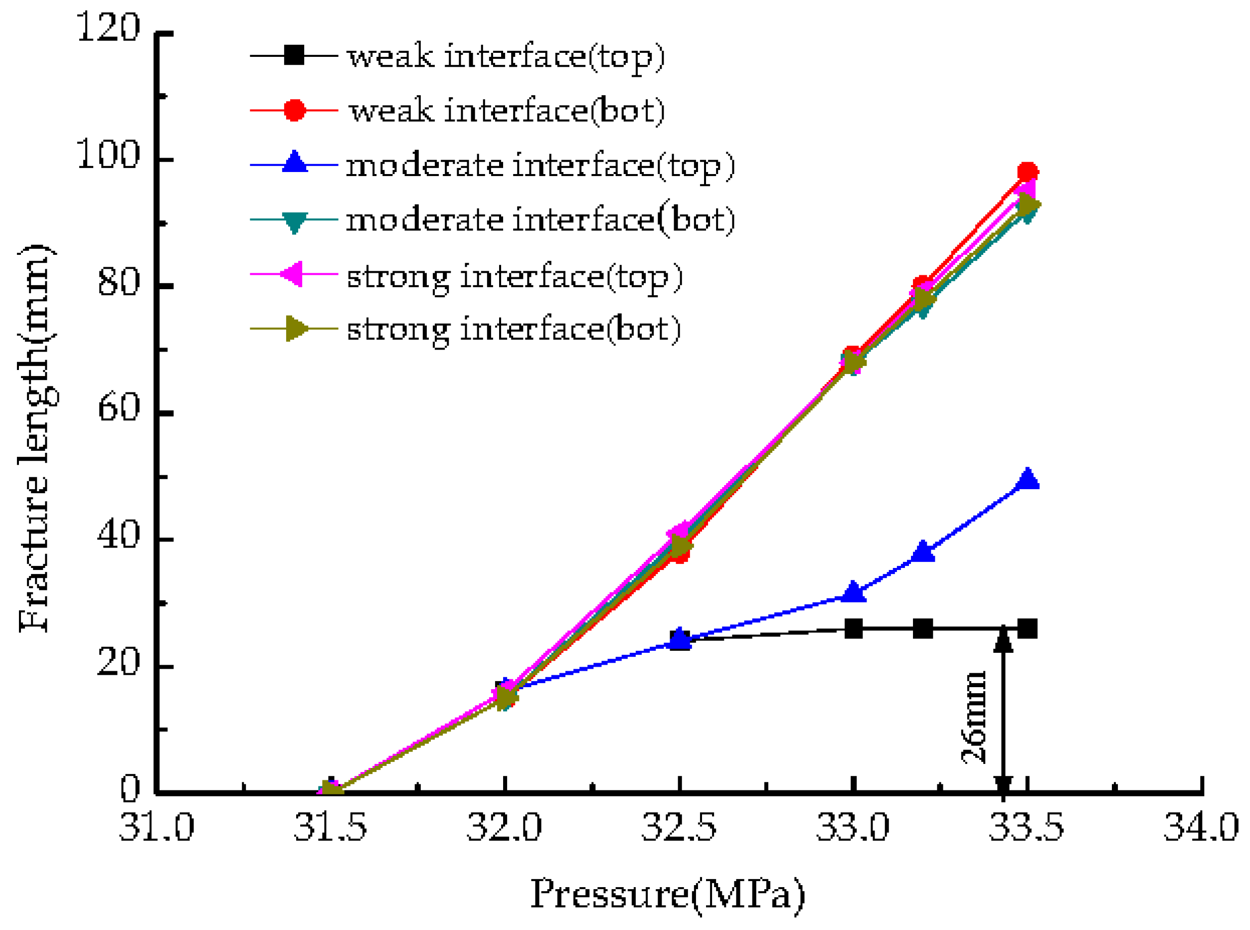
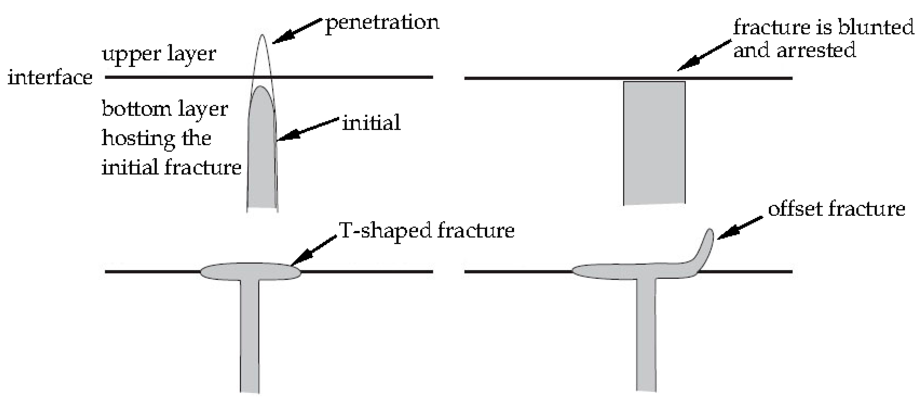
3.2.2. The Influence of Interface Strength on Hydro-Fracture Propagation

Clearly, besides in-situ stresses, fracture propagation across interface depends on many other factors, in which the interface properties play a key role in the interaction of the hydraulic fracture with the interface. To make a detailed investigation on the influence of interface properties on hydraulic fracture propagation, varying the interface properties while holding all of other material parameters and boundary conditions constant, another two cases (referred to as weak interface case and strong interface case) are considered. The properties for weak interface are E = 100 MPa, v = 0.45, c = 1.0 MPa and f_t = 0.1 MPa, while the properties for strong interface are E = 1000 MPa, v = 0.35, c = 5.0 MPa and f_t = 2.0 MPa. The other mechanical parameters are the same as those listed in Table 3. The applied constant confining stresses are σ_h = 13 MPa and σ_v = 20 MPa.

The numerical results for the two cases are presented in Figure 16. As a comparison, the numerical results of the case with moderate-strength interface are also listed in Figure 16. The overall fracturing patterns are similar to those in Figure 12, Figure 13 and Figure 14; the profiles of the hydraulic fracture are characterized by numerous deflections, branchings, and terminations or step-over. Upon intersecting the interface, a fluid-driven fracture can grow along it in either direction or in both directions by overcoming the higher vertical stress and the extra compressive stress from the interaction between the interface and fractures.

For the case with a weak interface, as a fracture propagates toward the interface, weak interface can open easily under interface tension. Debonding and subsequent opening of the interface occur when interface normal tensile stresses exceed the prescribed interface tensile strength, then fracture propagates forward along the interface. Finally the fracture is blunted and fully arrested in sandstone layer. While for the case with strong interface, since these strong interfaces neither open nor slide within the model, the interfaces are likely to be bonded or welded. As a fracture propagates toward an interface, tensile stresses smoothly develop across the interface. The high interface stiffness minimize elastic deformation along the interface so that the resulting behavior is limited to keeping close due to stresses that meet the prescribed interface opening criteria. As a result, the fracture directly propagates through the interface, although the fracture path is rough.

As is indicated above, the fractures may either become arrested or offset at the interface between two layers. Because for most cases, the interface is relatively weak comparing the properties of its adjacent layers, the stress barriers, resulted from the strongly contrasting stiffness, are very effective at hydro-fracture arrest. If there are (laminated) multilayers, most fractures either become arrested or offset at the layer interfaces, indicating that it is normally more difficult for fractures to propagate through such multilayers simultaneously. The mechanism of this phenomenon is same to that in many composite materials [69,70]. The only difference is that the sliding along interface is not considered in this study, because in fracture propagation driven by hydraulic pressure, the local interface opening, rather than sliding, is primarily responsible for the termination and step-over of fractures [1,71], although the hydro-fractures from and along frictional interfaces also have been investigated by some researchers [15].

Figure 17 shows the variation of fracture length with the increasing hydraulic pressure. For the case with a strong interface, the fractures on the top and bottom sides of the wellbore are generally symmetric. While for the other two cases, the growth of the top and bottom fractures shows is evidently asymmetric, particular for the case with a weak interface. To achieve the same fracture length, the higher fluid pressures are needed in latter two cases.

We investigated the potential for fracture propagation across, termination at, or step-over at a bedding interface by examining the fracturing process and associated stress evolution as the fracture approaches the interface. In general, there are four types of interaction between a fluid-driven fracture and a bedding interface within layered sedimentary rocks. Fractures can penetrate through the interface without any division of the fracture path. This type of crossing is what is implicitly assumed to occur by all current hydraulic fracture design models (the case with a higher deviatoric confining stress or the case with strong interface). In the opposite extreme case, the hydraulic fracture may be arrested or blunted at the interface (the case with a lower deviatoric confining stress or the case with weak interface). Between these above two extremes, a potential intermediate state is that the fracture is deflected into the interface plane and is divided into two branches (the case with a particular moderate deviatoric confining stress or the case with moderate-strength interface). If the interface is free of flaws, the fluid will invade it in the same way as an opening-mode hydraulic fracture growing along the horizontal interface, so that the vertical fracture eventually terminates at the interface, becoming a T-shaped fracture. Moreover, if there are flaws on the interface, potential re-initiation of a new fracture from one flaw will leave a step-over at the interface [1,56]. The numerical results are consistent with the conceptual modes of hydraulic fractures approaching interfaces, as sketched in Figure 18 [72].

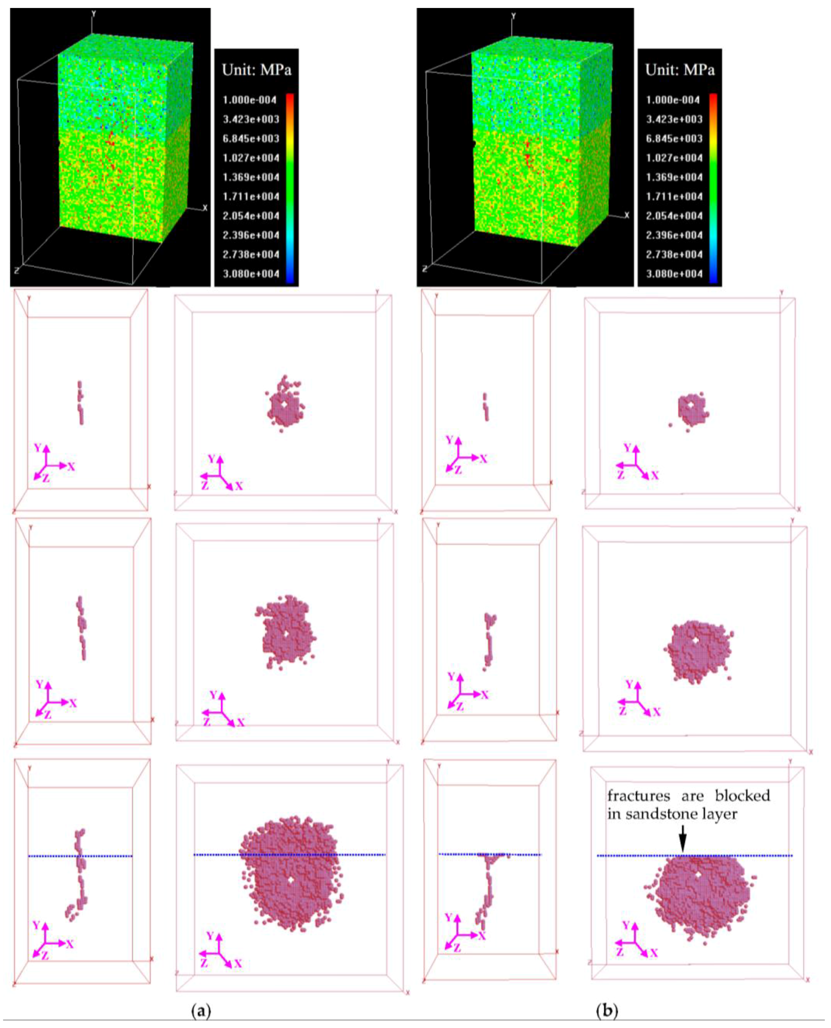
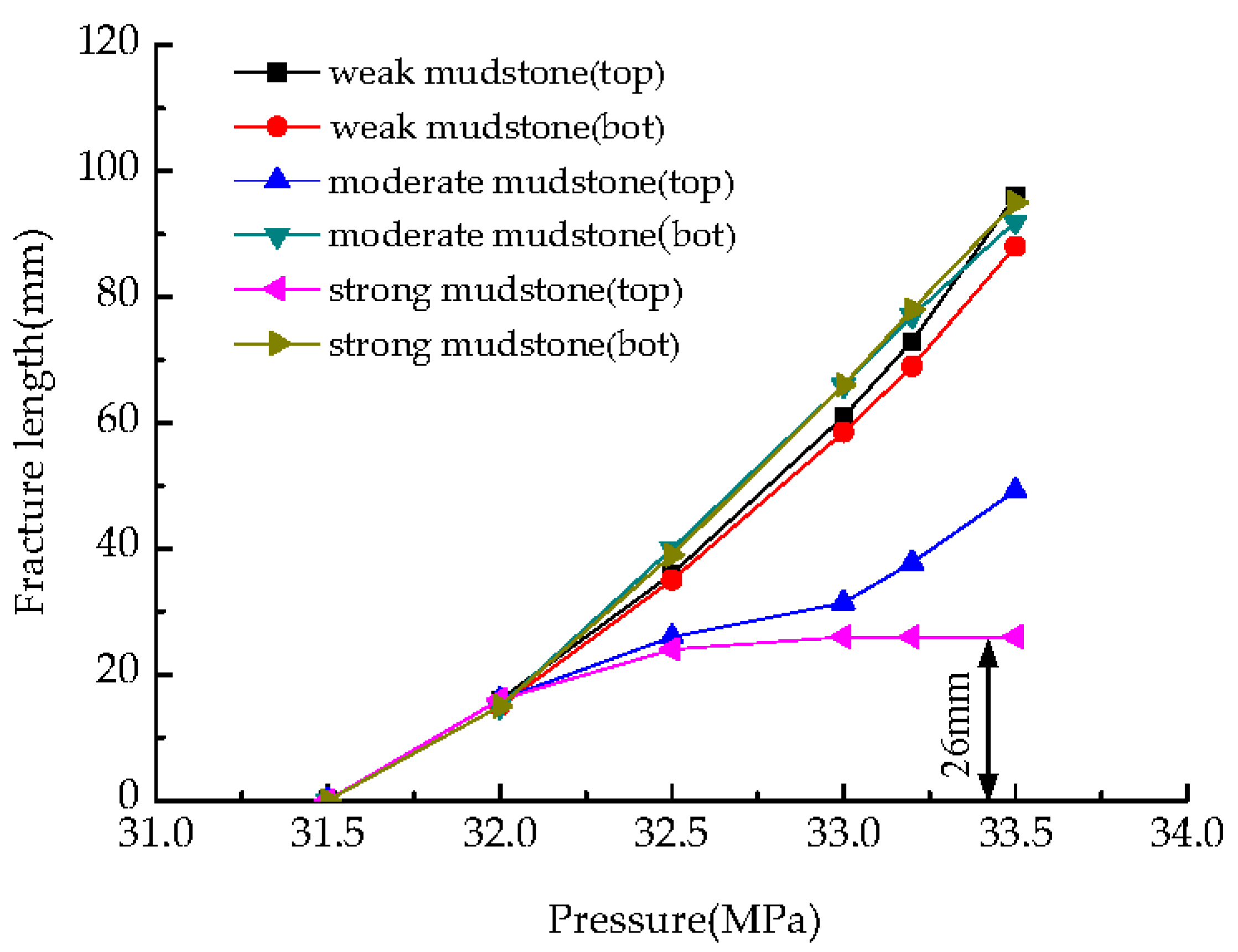
3.2.3. The Influence of Top Layer Strength on Hydro-Fracture Propagation

Complex morphology of hydro-fractures is caused by stress barrier, while the initiation and propagation hydro-fractures not only depend on the stress magnitude but also depend on the strength properties of the adjacent layers of the interface. To investigate the effect of the rock strata properties on the fracturing mode, another two cases (referred to as case with lower-strength top layer and the case with higher-strength top layer) were considered. In case with lower-strength top layer, the strength properties of the mudstone layer are assumed to be reduced by 50%, compared with those of the case shown in Figure 12 (the model shown in Figure 12 is referred to as the case with moderate-strength top layer), while in case with higher-strength top layer, the strength properties of the mudstone layer are increased by 50%. The other parameters were kept constant at the values listed in Table 3. The applied constant confining stresses are σ_h = 13 MPa and σ_v = 20 MPa.

Figure 19 shows the fracturing modes for these two cases. In case with lower-strength top layer, the fluid-driven fractures clearly propagate across the interfaces from the mudstone layer to mudstone layers and continue to propagate. By overcoming the higher vertical stress and the extra compressive stress generated from the interaction between the fractures, each fracture is initiated in a non-preferred direction, turns and twists during propagation, and tends to align itself with the preferred direction and plane.

In case with higher-strength top layer, the fluid-driven fractures are clearly blunted by the mudstone layer, although debonding and subsequent opening of the interface occurs. The strength of the mudstone layer is high enough that fractures only keep propagating along the interface and any new fractures along the mudstone side of the interface cannot initiate, then a T-shaped fracture is finally formed. In this case, because the interface in the model is an ideal interface, the fractures keep propagating along the interface. If the fractures stop propagating along the interface due to local heterogeneity of interface or some particular blocking measures in practical engineering, the fluid flow is then prevented from escaping along the interface and an either fracture step-over or fracture propagation across the interface may occur.

Figure 20 shows the variation of fracture length with the increasing hydraulic pressure. For the case with lower-strength mudstone layer, the fractures on the top and bottom sides of the wellbore are generally symmetric. While for the other two cases, the growth of the top and bottom fractures is evidently asymmetric, particular for the case with a higher-strength mudstone layer. The stronger top rock with higher toughness is found to efficiently resist fracture escaping, correspondingly, the higher fluid pressures are needed in the case.

4. Concluding Remarks

In this study, the RFPA code was applied to simulate the hydraulic fracturing mechanism in heterogeneous and layered rocks. Although the reality is often much more complex than that simulated by the applied numerical models, the study provided several interesting insights which lead to a better understanding of fracture initiation and propagation mechanisms associated with hydraulic fracturing. From the present numerical simulations, the following conclusions are derived.

Hydro-fracture propagation within a layered sequence of sedimentary rocks is controlled by changing in situ stresses, interface properties, and lithologies. There are four types of interaction between a hydro-fracture and a bedding interface within the layered sedimentary rocks. In the case with a higher deviatoric in situ stress or the case with strong interface between adjacent layers, the hydro-fracture is likely to penetrate through the interface without any branching or bifurcation of the fracture path. In the opposite extreme case, the hydro-fracture may be arrested or blunted at the interface. Between these above two extremes, a potential intermediate state is that the fracture is deflected into the interface plane and is divided into two branches. Then a blunted fracture or a T-shaped fracture may form.

It is important to consider the stress fluctuations induced by heterogeneity in case that fracturing process is conducted. The maximum tension stress is not the only consideration for fracture initiation, the distribution of the flaws is also important, i.e., heterogeneity is a key factor that influences the fracture pattern in modelling. For example, if there are flaws on the interface, potential re-initiation of a new fracture from one flaw may leave a step-over at the interface. The distance of step will be determined by the mechanics of stress transfer and factors involved in fracture initiation, such as the size and distribution of flaws near the interface.

The fracture propagation is influenced by the distribution of the inhibiting layers and out-of-plane growth of fractures from one unit to another, all of which have practical and economic implications for oil and gas recovery. The competition and interaction between fracture branches of a fluid-driven composite fracture result in complex fluid flow and fracture growth patterns. Discontinuous composite fracture segments resulting from out-of-plane growth of fractures provide a less permeable path for fluids, gas, and oil than a continuous planar composite fracture. Although many issues need to be further clarified, the results provided here can assist in the understanding of the development of hydraulic fracture networks in nature. The fracture initiation, propagation, and coalescence are represented visually during the whole hydraulic fracturing process. These results provide supplementary information on the stress distribution and failure-induced stress redistribution, and show in detail the propagation of the fracture zone and the interaction of the fractures, which are impossible to be observed in field and are difficult to be considered with static stress analysis approaches.

Based on the modelling results, several additional factors influencing the hydraulic fracturing will be considered in future studies. For example, non-Newtonian fluids will be considered in a future model. The fluid used in this study is water. Although the non-Newtonian fluid behaviour is not expected to alter the overall findings of this study, the Newtonian assumption may affect the fracture width and thereby influence the fracture volume and injection pressure. In addition, the mechanical properties of mudstone are relatively more prone to be degraded subjected to the soaking of fluid flow. Although most of mudstone in beach-bar sandstone reservoirs have experienced diagenetic metamorphism [73], there is a need to consider the degradation law of mudstone for more accurate modelling of the fracturing process.

References

1. Cooke, M.L.; Underwood, C.A. Fracture termination and step-over at bedding interfaces due to frictional slip and interface opening. J. Struct. Geol. 2001, 23, 223–238. [Google Scholar] [CrossRef]
2. Clifton, H.E. Supply, segregation, successions, and significance of shallow marine conglomeratic deposits. Bull. Can. Pet. Geol. 2003, 51, 370–388. [Google Scholar] [CrossRef]
3. Wang, Y.S.; Liu, H.M.; Gao, Y.J.; Tian, M.R.; Tang, D. Sandbody genesis and hydrocarbon accumulation mechanism of beach-bar reservoir in faulted-lacustrine-basins: A case study from the upper of the fourth member of Shahejie Formation, Dongying Sag. Front. Earth Sci. 2012, 19, 100–107. [Google Scholar]
4. Li, L.C.; Wang, L.; Xia, Y.J.; Yang, T. The Feasibility of Developing Reserves in Beach-Bar Sandstone Reservoirs; Research Report of Oil Production Technology Research Institute, Shengli Oilfield Branch Company: Dongying, China, 2013. [Google Scholar]
5. Warpinski, N.R.; Teufel, L.W. Influence of geologic discontinuities on hydraulic fracture propagation. J. Petrol. Technol. 1987, 39, 209–220. [Google Scholar] [CrossRef]
6. Jeffrey, R.G. A symmetrically propped hydraulic fractures. SPE Prod. Facil. 1966, 11, 244–249. [Google Scholar]
7. Zhang, X.; Jeffrey, R.G.; Thiercelin, M. Deflection and propagation of fluid-driven fractures at frictional bedding interfaces: A numerical investigation. J. Struct. Geol. 2007, 29, 396–410. [Google Scholar] [CrossRef]
8. Han, G. Natural Fractures in Unconventional Reservoir Rocks: Identification, Characterization, and its Impact to Engineering Design. In Proceeding of the Conference on American Rock Mechanics, ARMA, San Francisco, CA, USA, 26–29 June 2011; pp. 11–509.
9. Jeffrey, R.G.; Weber, C.R.; Vlahovic, W.; Enever, J.R. Hydraulic fracturing experiments in the great northern coal seam. In Proceedings of the 1994 SPE Asia Pacific Oil & Gas Conference, Melbourne, Austrila, 25–27 January 1994.
10. Helgeson, D.E.; Aydin, A. Characteristics of joint propagation across layer interfaces in sedimentary rocks. J. Struct. Geol. 1991, 13, 897–911. [Google Scholar] [CrossRef]
11. Gudmundsson, A.; Brenner, S.L. How hydro-fractures become arrested. Terra Nova 2001, 13, 456–462. [Google Scholar] [CrossRef]
12. Gudmundsson, A.; Fjeldskaar, I.; Brenner, S.L. Propagation pathways and fluid transport of hydro-fractures in jointed and layered rocks in geothermal fields. J. Volcanol. Geotherm. Res. 2002, 116, 257–278. [Google Scholar] [CrossRef]
13. Gudmundsson, A.; Simmenes, T.H.; Larsen, B.; Philipp, S.L. Effects of internal structure and local stresses on fracture propagation, deflection, and arrest in fault zones. J. Struct. Geol. 2010, 32, 1643–1655. [Google Scholar] [CrossRef]
14. Adachi, J.; Siebrits, E.; Peirce, A.; Desroches, J. Computer simulation of hydraulic fractures. Int. J. Rock Mech. Min. Sci. 2007, 44, 739–757. [Google Scholar] [CrossRef]
15. Zhang, X.; Jeffrey, R.G.; Thiercelin, M. Escape of fluid-driven fractures from frictional bedding interfaces: A numerical study. J. Struct. Geol. 2008, 30, 478–490. [Google Scholar] [CrossRef]
16. Zhang, Z.; Li, X.; He, J.; Wu, Y.; Zhang, B. Numerical analysis on the stability of hydraulic fracture propagation. Energies 2015, 8, 9860–9877. [Google Scholar] [CrossRef]
17. Zhang, Z.; Li, X.; Yuan, W.; He, J.; Li, G.; Wu, Y. Numerical Analysis on the Optimization of Hydraulic Fracture Networks. Energies 2015, 8, 12061–12079. [Google Scholar] [CrossRef]
18. Ma, S.; Guo, J.C.; Li, L.L.; Xia, Y.J.; Yang, T. Experimental and numerical study on fracture propagation near open-hole horizontal well under hydraulic pressure. Eur. J. Environ. Civ. Eng. 2015. [Google Scholar] [CrossRef]
19. Wen, X.L. Using horizontal well fracturing technology to improve reservoir reserve development ratio in the beach-bar sandstone reservoirs with low permeability. China Pet. Chem. Stand. Qual. 2012, 32, 1–2. [Google Scholar]
20. Tang, C.A.; Tham, L.G.; Lee, P.K.K.; Yang, T.H.; Li, L.C. Coupled analysis of flow, stress and damage (FSD) in rock failure. Int. J. Rock. Mech. Min. Sci. 2002, 39, 477–489. [Google Scholar] [CrossRef]
21. Li, L.C.; Tang, C.A.; Li, G.; Wang, S.Y.; Liang, Z.Z.; Zhang, Y.B. Numerical simulation of 3D hydraulic fracturing based on an improved flow-stress-damage model and a parallel FEM technique. Rock Mech. Rock Eng. 2012, 45, 801–818. [Google Scholar] [CrossRef]
22. Biot, M.A. General theory of three-dimensional consolidation. J. Appl. Phys. 1941, 12, 155–164. [Google Scholar] [CrossRef]
23. Weibull, W.A. A statistical distribution function of wide applicability. J. Appl. Mech. 1951, 18, 293–297. [Google Scholar]
24. Tang, C.A.; Liu, H.; Lee, P.K.K.; Tsui, Y.; Tham, L.G. Numerical studies of the influence of microstructure on rock failure in uniaxial compression. Part I: Effect of heterogeneity. Int. J. Rock Mech. Min. Sci. 2000, 37, 555–569. [Google Scholar] [CrossRef]
25. Wong, T.F.; Wong, R.H.C.; Chau, K.T.; Tang, C.A. Microcrack statistics, Weibull distribution and micromechanical modeling of compressive failure in rock. Mech. Mater. 2006, 38, 664–681. [Google Scholar] [CrossRef]
26. Zhu, W.L.; Wong, T.F. Network modeling of the evolution of permeability and dilatancy in compact rock. J. Geophys. Res. 1999, 104, 2963–2971. [Google Scholar] [CrossRef]
27. Yale, D.P.; Lyons, S.L.; Qin, G. Coupled geomechanics-fluid flow modeling in petroleum reservoirs: Coupled versus uncoupled response. In Pacific Rocks; Girard, J., Liebman, M., Breed, C., Doe, T., Eds.; Balkema: Rotterdam, The Netherlands, 2000; pp. 137–144. [Google Scholar]
28. Lemaitre, J.; Desmorat, R. Engineering Damage Mechanics: Ductile, Creep, Fatigue and Brittle Failures; Springer-Verlag: Berlin, Germany, 2005. [Google Scholar]
29. Murakami, S. Continuum Damage Mechanics—A Continuum Mechanics Approach to the Analysis of Damage and Fracture; Springer: New York, NY, USA, 2012. [Google Scholar]
30. Mazars, J.; Pijaudier-Cabot, G. Continuum damage theory—Application to concrete. J. Eng. Mech. ASCE 1987, 115, 345–365. [Google Scholar] [CrossRef]
31. Shimizu, H.; Murata, S.; Ishida, T. The distinct element analysis for hydraulic fracturing in hard rock considering fluid viscosity and particle size distribution. Int. J. Rock Mech. Min. Sci. 2011, 48, 712–727. [Google Scholar] [CrossRef]
32. Petit, J.P.; Barquins, M. Can natural faults propagate under mode II conditions? Tectonics 1988, 7, 1243–1256. [Google Scholar] [CrossRef]
33. Tang, C.A.; Kou, S.Q. Crack propagation and coalescence in brittle materials under compression. Eng. Fract. Mech. 1998, 61, 311–324. [Google Scholar] [CrossRef]
34. Healy, D.; Jones, R.R.; Holdsworth, R.E. Three-dimensional brittle shear fracturing by tensile crack interaction. Nature 2006, 439. [Google Scholar] [CrossRef] [PubMed]
35. Li, G.; Tang, C.A.; Li, L.C.; Li, H. An unconditionally stable explicit and precise multiple timescale finite element modeling scheme for the fully coupled hydro-mechanical analysis of saturated poroelastic media. Comput. Geotech. 2016, 71, 69–81. [Google Scholar] [CrossRef]
36. Zhuang, X.; Huang, R.; Liang, C.; Rabczuk, T. A coupled thermo-hydro-mechanical model of jointed hard rock for compressed air energy storage. Math. Probl. Eng. 2014, 179169. [Google Scholar] [CrossRef]
37. Lee, S.H.; Ghassemi, A. Three-dimensional thermo-poro-mechanical modeling of well stimulation and induced microseismicity. In Proceedings of the 45th US Rock Mechanics/Geomechanics Symposium, San Francisco, CA, USA, 26–29 June 2011.
38. Rawal, C.; Ghassemi, A. Poroelastic rock failure analysis around multiple hydraulic fractures using a BEM/FEM model. In Proceedings of the 45th US Rock Mechanics/Geomechanics Symposium, San Francisco, CA, USA, 26–29 June 2011.
39. Rabczuk, T.; Belytschko, T. A three dimensional large deformation meshfree method for arbitrary evolving cracks. Comput. Methods Appl. M 2007, 196, 2777–2799. [Google Scholar] [CrossRef]
40. Rabczuk, T.; Zi, G.; Bordas, S.; Nguyen-Xuan, H. A simple and robust three-dimensional cracking-particle method without enrichment. Comput. Methods Appl. M 2010, 199, 2437–2455. [Google Scholar] [CrossRef]
41. Rabczuk, T.; Bordas, S.; Zi, G. A three-dimensional meshfree method for continuous multiple crack initiation, nucleation and propagation in statics and dynamics. Comput. Mech. 2007, 40, 473–495. [Google Scholar] [CrossRef]
42. Zhuang, X.; Augarde, C.; Mathisen, K. Fracture modelling using meshless methods and level sets in 3D: Framework and modelling. Int. J. Numer. Meth. Eng. 2012, 92, 969–998. [Google Scholar] [CrossRef]
43. Budarapu, P.; Gracie, R.; Bordas, S.; Rabczuk, T. An adaptive multiscale method for quasi-static crack growth. Comput. Mech. 2014, 53, 1129–1148. [Google Scholar] [CrossRef]
44. Yang, T.H.; Zhu, W.C.; Yu, Q.L.; Liu, H.L. The role of pore pressure during hydraulic fracturing and implications for groundwater outbursts in mining and tunnelling. Hydrogeol. J. 2011, 19, 995–1008. [Google Scholar] [CrossRef]
45. Tang, C.A.; Tham, L.G.; Wang, S.H.; Liu, H.; Li, W.H. A numerical study of the influence of heterogeneity on the strength characterization of rock under uniaxial tension. Mech. Mater. 2007, 39, 326–339. [Google Scholar] [CrossRef]
46. Cai, M.F.; He, M.C.; Liu, D.Y. Rock Mechanics and Engineering; Science Press: Beijing, China, 2002. [Google Scholar]
47. Malvar, L.J.; Fourney, M.E. A three dimensional application of the smeared crack approach. Eng. Fract. Mech. 1990, 35, 251–260. [Google Scholar] [CrossRef]
48. Pietruszczak, S.; Xu, G. Brittle response of concrete as a localization problem. Int. J. Solids Struct. 1995, 32, 1517–1533. [Google Scholar] [CrossRef]
49. Pearce, C.J.; Thavalingam, A.; Liao, Z.; Bicanic, N. Computational aspects of the discontinuous deformation analysis framework for modeling concrete fracture. Eng. Fract. Mech. 2000, 65, 283–298. [Google Scholar] [CrossRef]
50. Yuan, S.C.; Harrison, J.P. Development of a hydro-mechanical local degradation approach and its application to modelling fluid flow during progressive fracturing of heterogeneous rocks. Int. J. Rock Mech. Min. Sci. 2005, 42, 961–984. [Google Scholar] [CrossRef]
51. Ma, G.W.; Wang, X.J.; Ren, F. Numerical simulation of compressive failure of heterogeneous rock-like materials using SPH method. Int. J. Rock Mech. Min. Sci. 2011, 48, 353–363. [Google Scholar] [CrossRef]
52. Hubbert, M.K.; Willis, D.G. Mechanics of hydraulic fracturing. Trans AIME 1957, 210, 153–166. [Google Scholar]
53. Haimson, B.C.; Fairhurst, C. Initiation and extension of hydraulic fractures in rock. Soc. Pet. Eng. J. 1967, 7, 310–318. [Google Scholar] [CrossRef]
54. Medlin, W.L.; Fitch, J.L. Abnormal treating pressures in MHF treatments. In Proceedings of the 58th SPE Annual Technical Conference and Exhibition, San Francisco, CA, USA, 5–8 October 1983. SPE 12108.
55. Hossain, M.M.; Rahman, M.K. Numerical simulation of complex fracture growth during tight reservoir stimulation by hydraulic fracturing. J. Pet. Sci. Eng. 2008, 60, 86–104. [Google Scholar] [CrossRef]
56. Erdogan, F.; Biricikoglu, V. Two bonded half planes with a crack going through the interface. Int. J. Eng. Sci. 1973, 11, 745–766. [Google Scholar] [CrossRef]
57. Pollard, D.D.; Aydin, A. Progress in understanding joints over the last century. Geol. Soc. Am. Bull. 1988, 100, 1181–1204. [Google Scholar] [CrossRef]
58. Zhu, W.C.; Tang, C.A.; Wang, S.Y. Numerical study on the influence of mesomechanical properties on macroscopic fracture of concrete. Struct. Eng. Mech. 2005, 19, 519–533. [Google Scholar] [CrossRef]
59. Li, L.C.; Yang, T.H.; Liang, Z.Z.; Zhu, W.C.; Tang, C.A. Numerical investigation of groundwater outbursts near faults in underground coal mines. Int. J. Coal Geol. 2011, 85, 276–288. [Google Scholar]
60. Goodman, R.E. Introduction to Rock Mechanics; John Wiley: New York, NY, USA, 1989. [Google Scholar]
61. Li, L.C.; Meng, Q.M.; Li, G.; Wang, S.Y. A numerical investigation of the hydraulic fracturing behavior of conglomerate in Glutenite formation. Acta Geotech. 2013. [Google Scholar] [CrossRef]
62. Bonafede, M.; Rivalta, E. The tensile dislocation problem in a layered elastic medium. Geophys. J. Int. 1999, 136, 341–356. [Google Scholar] [CrossRef]
63. Fairhurst, C. On the validity of the Brazilian test for brittle materials. Int. J. Rock Mech. Min. Sci. 1964, 1, 535–546. [Google Scholar] [CrossRef]
64. Gross, M.R. The origin and spacing of cross-joints: Examples from the Monterey Formation, Santa Barbara, California. J. Struct. Geol. 1993, 15, 737–751. [Google Scholar] [CrossRef]
65. Teufel, L.W.; Clark, J.C. Hydraulic fracture propagation in layered rocks: Experimental studies of fracture containment. Soc. Pet. Eng. J. 1984, 24, 19–34. [Google Scholar] [CrossRef]
66. Renshaw, C.E.; Pollard, D.D. An experimentally verified criterion for propagation across unbonded frictional interfaces in brittle, linear elastic materials. Int. J. Rock Mech. Min. Sci. Geomech. Abstr. 1995, 32, 237–249. [Google Scholar] [CrossRef]
67. Zhao, S.X.; Yu, H.J. Economical production technologies research and application of ultra low permeability beach-bar sand reservoirs. Pet. Geol. Recovery Effic. 2009, 16, 96–98. [Google Scholar]
68. Wang, F.Y.; Wu, X.D. Technology of water injection for beach-bar sand reservoirs with low permeability in Block Fan 151. Fault-Block Oil Gas Field 2010, 17, 596–598. [Google Scholar]
69. Chawla, K.K. Composite Materials: Science and Engineering; Springer: New York, NY, USA, 1998. [Google Scholar]
70. Larsen, B.; Grunnaleite, I.; Gudmundsson, A. How fracture systems affect permeability development in shallow-water carbonate rocks: An example from the Gargano Peninsula, Italy. J. Struct. Geol. 2010, 32, 1212–1230. [Google Scholar] [CrossRef]
71. Charlez, P.A. Rock Mechanics: Petroleum Applications; Editions Technip: Paris, France, 1997; Volume 2. [Google Scholar]
72. Thiercelin, M.; Roegiers, J.C.; Boone, T.J.; Ingraffea, A.R. An investigation of the material parameters that govern the behavior of fractures approaching rock interfaces. In Proceedings of the LSRM Sixth International Congress of Rock Mechanics, Montreal, QC, Canada, 30 August–3 September 1987; pp. 263–269.
73. Li, C.Q. Investigation on the New Technology of Developing Reserves in Beach-Bar Sandstone Reservoirs; Research Report of Oil Production Technology Research Institute, Shengli Oilfield Branch Company: Dongying, China, 2009. [Google Scholar]
Figure 1. The typical multiple rock layers and the observed complex fracturing modes in field, (a) the sedimentary characteristics of bar sand subfacies and beach sand subfacies in one of beach-bar sandstone reservoirs in Shengli Oilfield of China [3]; (b) outcrop of a shale formation, where the horizontal beddings are cut by the vertical fractures (denoted by red dashed line) to form fracture networks, Well A and B are the conceptual vertical and horizontal wells [8]; and (c) a hydraulic fracture that grew vertically in a coal seam and horizontally along the interface between the coal and the roof rock (the hydro-fracture is shown in yellow and the black arrows represent the fracturing direction) [9].
Energies 09 00169 g001
Figure 2. The fracture profile of rock sample in laboratory experiment on hydraulic fracturing near horizontal wells (well trajectory is denoted by the red dashed line) [18].
Energies 09 00169 g002
Figure 3. Elastic-brittle damage constitutive law of element subject to uniaxial stress, (a) the case under uniaxial tensile stress; (b) the case under uniaxial compressive stress.
Energies 09 00169 g003
Figure 4. Sketch of the numerical model for the hydraulic fracturing near a horizontal well (two different colors in the block represent different rocks: the top is mudstone and the bottom is sandstone).
Energies 09 00169 g004
Figure 5. The Mohr-Coulomb envelopes of the mudstone and sandstone in the beach-bar sandstone reservoir, (a) mudstone and (b) sandstone.
Energies 09 00169 g005
Figure 6. The hydraulic fracturing process in Case III, (a) elastic modulus; (b) minimum principal stress; (c) the evolution of minimum principal stress (a vertical section along the horizontal well); (d) the propagation of fracture: a side view in X-Y plane; and (e) the propagation of fracture: a side view in Y-Z plane (Note: in this model, the mudstone is not considered, i.e., the model is only composed of sandstone).
Energies 09 00169 g006
Figure 7. Breakdown pressure under the different confining stresses.
Energies 09 00169 g007
Figure 8. The fracture profile in the numerical models considering mudstone layer with different strength, (a) the layered model in which the mudstone layer has a normal strength (Case VI); (b) the layered model in which the mudstone layer has a higher strength (Case VII) (the two screen shots shown at the top of the figure show the vertical section view along wellbore, in which the colors indicate the relative magnitude of the elastic modulus of the mesoscopic elements).
Energies 09 00169 g008
Figure 9. The model configuration for the cases with an interface, (a) the geometrical dimensions of the numerical model; (b) Sketch of the numerical model presented with the relative magnitude of the elastic modulus of the mesoscopic elements, a brighter shade of grey corresponds to a higher Young’s modulus.
Energies 09 00169 g009aEnergies 09 00169 g009b
Figure 10. The numerically obtained minimum principal stress for case with confining stress σvh = 20:13, (a) the fluid pressure distribution; (b) the visualized stress fields presented with numerical photoelasticity when the heterogeneity index m = 100; and (c) the visualized stress fields presented with numerical photoelasticity when the heterogeneity index m = 2.5.
Energies 09 00169 g010
Figure 11. The minimum principal stress along the top of the interface for cases with different confining stresses.
Energies 09 00169 g011
Figure 12. Numerical results of the hydraulic fracturing process for case with confining stress σvh = 20:13. (a) The hydraclic fracturing process presented with Young’s modulus: (a1) fracture is initiated, (a2) fracture is blunted; (a3) an offset fracture is initiated; (a4) fracture passes the interface. And (b) the hydraclic fracturing process presented with the minimum principal stress: (b1) fracture is initiated; (b2) fracture is blunted; (b3) an offset fracture is initiated; (b4) fracture passes the interface.
Energies 09 00169 g012
Figure 13. Numerical results of the hydraulic fracturing process for case with confining stress σvh = 20:8. (a) The hydraclic fracturing process presented with Young’s modulus: (a1) fracture is initiated; (a2) fracture reaches the interface; (a3) fracture passes the interface directly. And (b) the hydraclic fracturing process presented with the minimum principal stress: (b1) fracture is initiated; (b2) fracture reaches the interface; (b3) fracture passes the interface directly.
Energies 09 00169 g013
Figure 14. Numerical results of the hydraulic fracturing process for case with confining stress σvh = 20:8. (a) The hydraclic fracturing process presented with Young’s modulus: (a1) fracture reaches the interface; (a2) fracture is blunted; (a3) a T-shaped fracture is formed. And (b) the hydraclic fracturing process presented with the minimum principal stress: (b1) fracture reaches the interface; (b2) fracture is blunted; (b3) a T-shaped fracture is formed.
Energies 09 00169 g014
Figure 15. Variation of fracture length with the hydraulic pressure for cases with different confining stresses.
Energies 09 00169 g015
Figure 16. Numerical results of the hydraulic fracturing process for cases with different interface strength. (a) The case with weak interface: (a1) fracture reaches the interface; (a2) fracture is blunted; (a3) a T-shaped fracture is formed. (b) The case with moderate-strength interface: (b1) fracture reaches the interface; (b2) an offset fracture is initiated; (b3) fracture passes the interface. And (c) the case with strong interface: (c1) fracture reaches the interface; (c2) fracture passes the interface directly; (c3) fracture keeps propagating.
Energies 09 00169 g016
Figure 17. Variation of fracture length with the hydraulic pressure for cases with different interface strength.
Energies 09 00169 g017
Figure 18. The conceptual mode of four types of interaction between hydraulic fractures and interfaces [72].
Energies 09 00169 g018
Figure 19. Numerical results of the hydraulic fracturing process for cases with different mudstone strength. (a) the case with weak top layer: (a1) fracture reaches the interface; (a2) fracture passes the interface directly; (a3) fracture keeps propagating. (b) The case with moderate-strength top layer: (b1) fracture reaches the interface; (b2) an offset fracture is initiated; (b3) fracture passes the interface. And (c) the case with strong top layer: (c1) fracture reaches the interface; (c2) fracture is blunted; (c3) a T-shaped fracture is formed.
Energies 09 00169 g019
Figure 20. Variation of fracture length with the hydraulic pressure for cases with different mudstone strength.
Energies 09 00169 g020