
Improved Spatio-Temporal Linear Models for Very Short-Term Wind Speed Forecasting


Abstract
:1. Introduction
2. Multi-Channel Wind Data and Linear Prediction Models
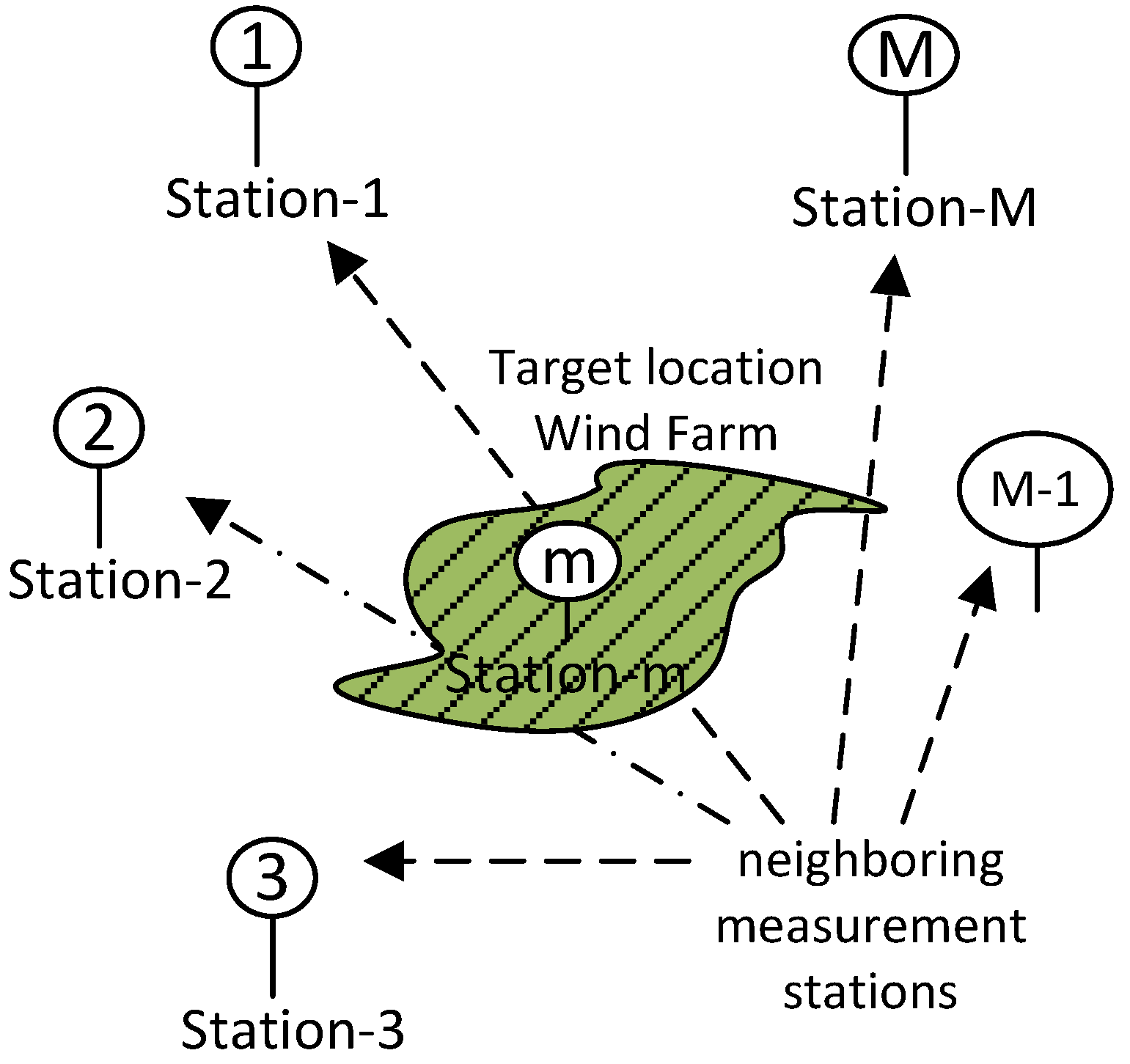
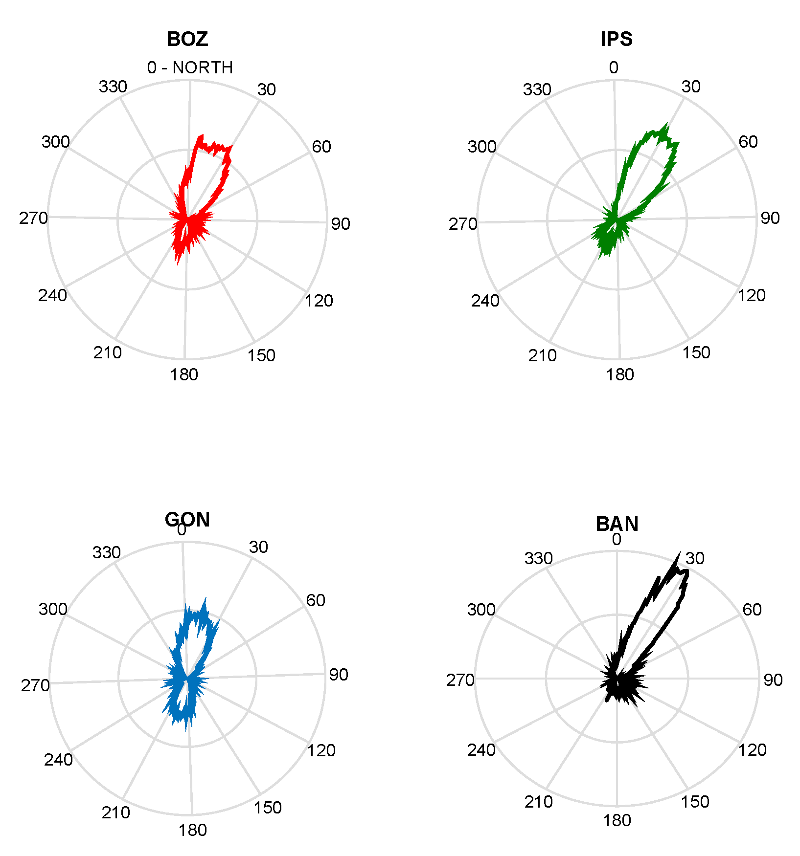
2.1. Multi-Channel Wind Data
2.2. Multi-Channel Linear Prediction Models
2.3. Multi-Channel Linear Prediction Coefficient Estimation
3. Data and Test Results
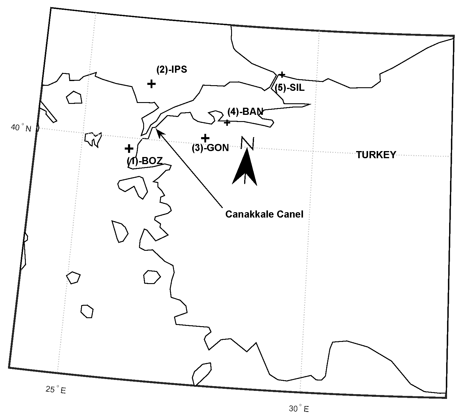
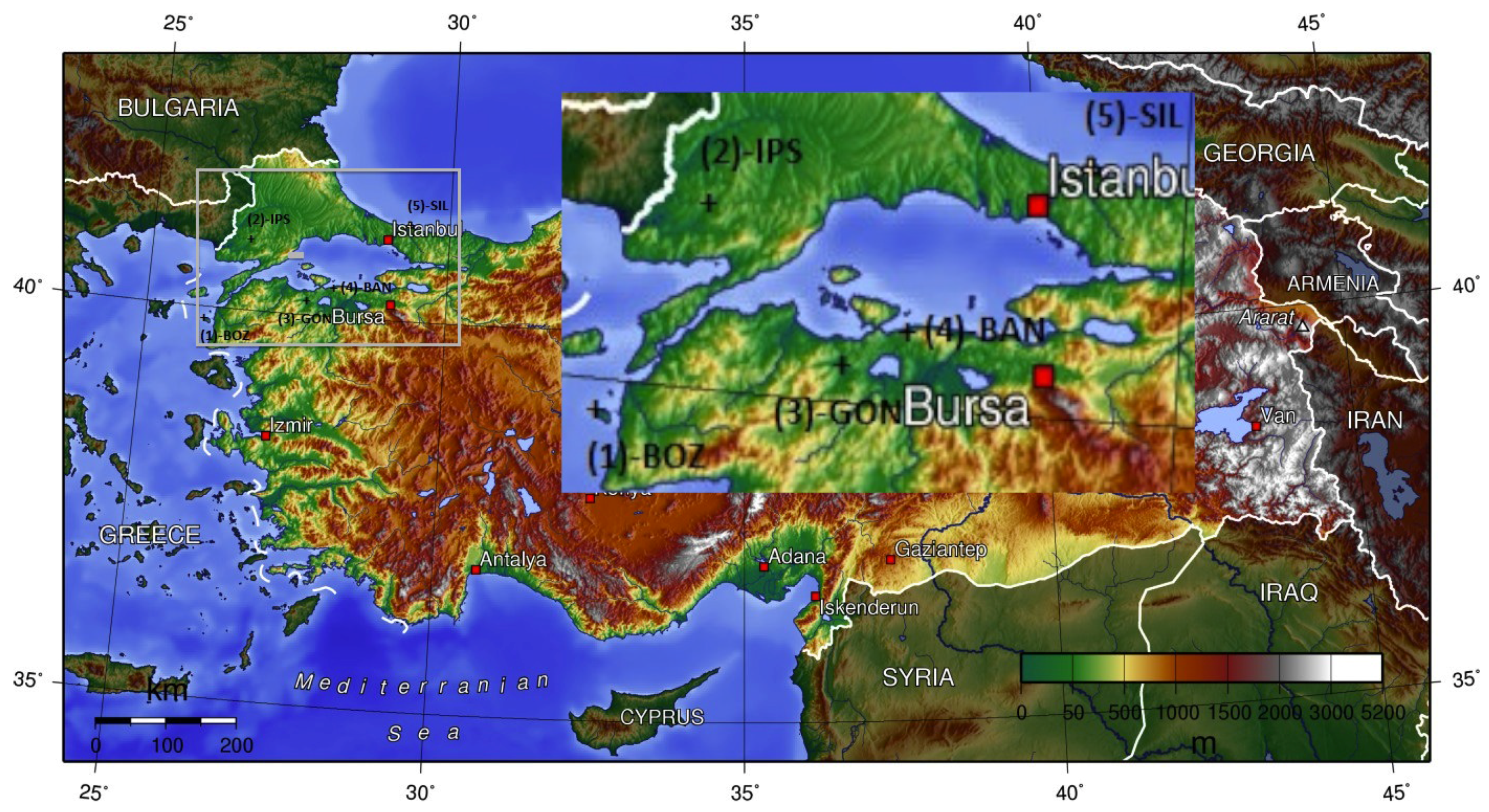
3.1. Data Set
3.2. Test Results
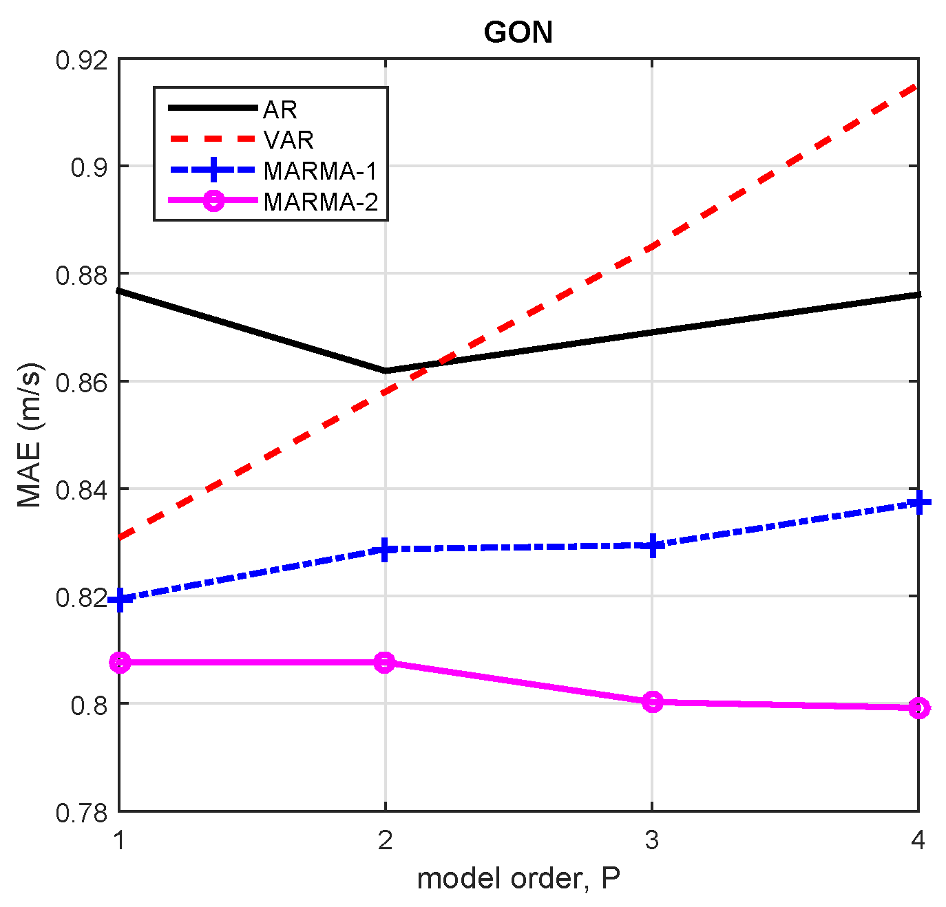
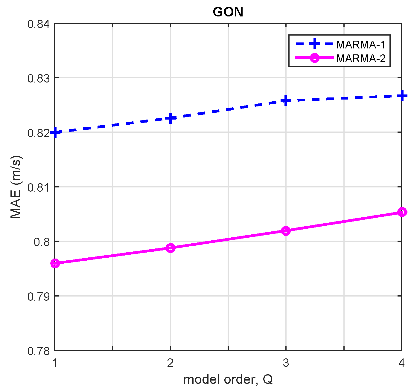
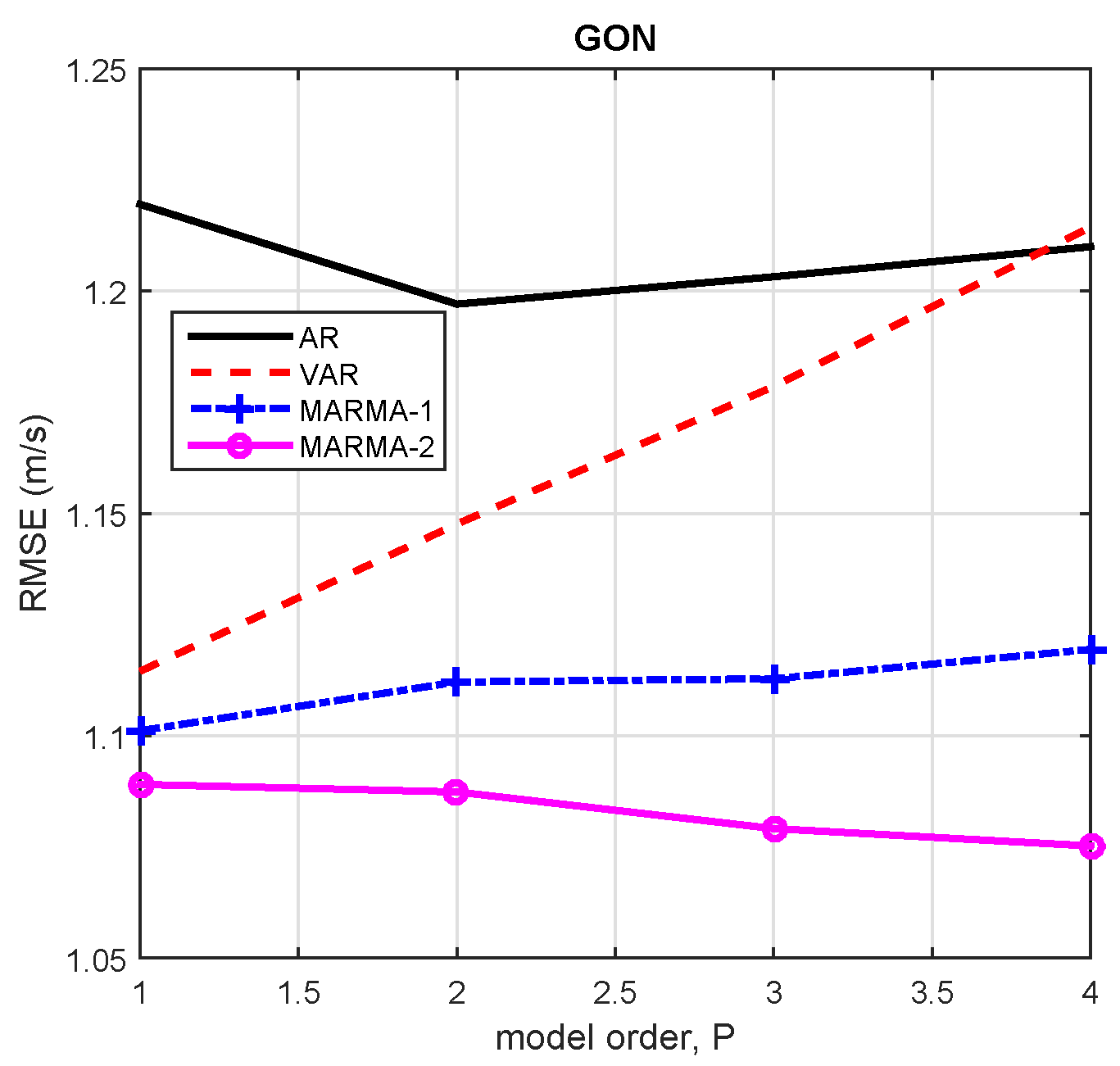
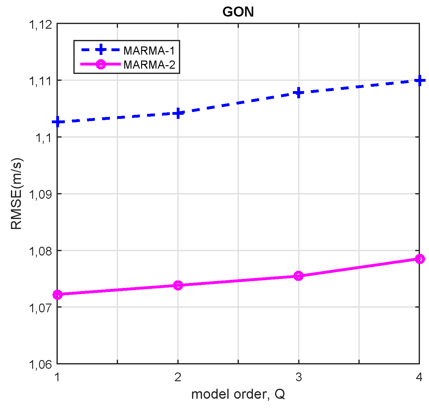
3.2.1. Model Order
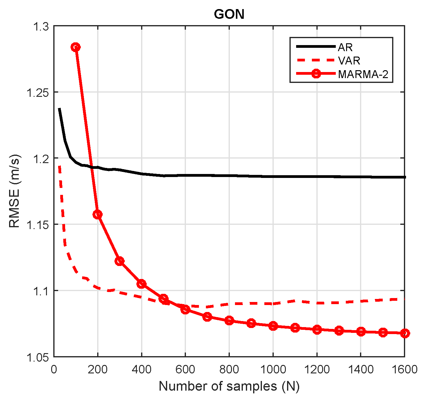
3.2.2. Number of Samples
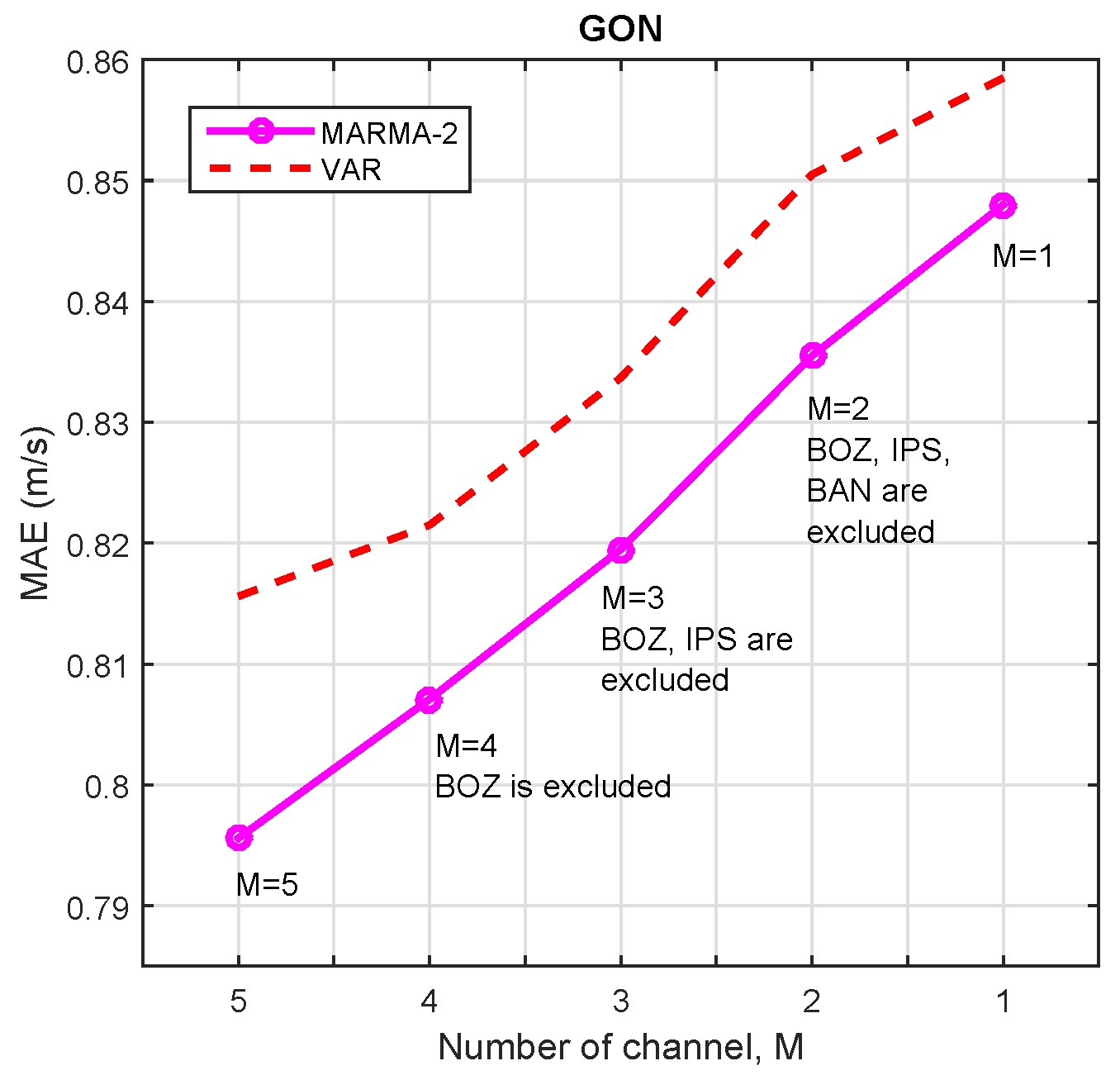
3.2.3. Number of Channels
3.2.4. Forecasting Results
4. Conclusions
Acknowledgments
Conflicts of Interest
References
- Filik, Ü.B.; Filik, T.; Gerek, Ö.N. New electric transmission systems—Experiences from Turkey. In The Handbook of Clean Energy Systems; Yan, J.Y., Ed.; John Wiley and Sons Ltd: New York, NY, USA, 2015; Volume 4, pp. 1981–1994. [Google Scholar]
- Filik, Ü.B.; Gerek, Ö.N.; Kurban, M. A novel modeling approach for hourly forecasting of long-term electric energy demand. Energy Convers. Manag. 2011, 52, 199–211. [Google Scholar]
- Moldan, B.; Janouskova, S.; Hak, T. How to understand and measure environmental sustainability: Indicators and targets. Ecol. Indic. 2012, 17, 4–13. [Google Scholar] [CrossRef]
- Farhangi, H. The path of a smart grid. IEEE Power Energy Mag. 2010, 8, 18–28. [Google Scholar] [CrossRef]
- Tastu, J.; Pinson, P.; Trombe, P.J.; Madsen, H. Probabilistic forecasts of wind power generation accounting for geographically dispersed information. IEEE Trans. Smart Grid 2014, 5, 480–489. [Google Scholar] [CrossRef]
- Bracale, A.; De Falco, P. An Advanced Bayesian Method for Short-Term Probabilistic Forecasting of the Generation of Wind Power. Energies 2015, 8, 10293–10314. [Google Scholar] [CrossRef]
- Lei, M.; Shiyan, L.; Jiang, C.W.; Liu, H.L.; Zhang, Y. A review on the forecasting of wind speed and generated power. Renew. Sustain. Energy Rev. 2009, 13, 915–920. [Google Scholar] [CrossRef]
- Zhu, X.X.; Genton, M.G. Short Term Wind Speed Forecasting for Power System Operations. Int. Stat. Rev. 2012, 80, 2–23. [Google Scholar] [CrossRef]
- De Giorgi, M.G.; Campilongo, S.; Ficarella, A.; Congedo, P.M. Comparison Between Wind Power Prediction Models Based on Wavelet Decomposition with Least-Squares Support Vector Machine (LS-SVM) and Artificial Neural Network (ANN). Energies 2014, 7, 5251–5272. [Google Scholar] [CrossRef]
- Jung, J.; Broadwater, R.P. Current status and future advances for wind speed and power forecasting. Renew. Sustain. Energy Rev. 2014, 31, 762–777. [Google Scholar] [CrossRef]
- Zhang, Y.; Wang, J.X.; Wang, X.F. Review on probabilistic forecasting of wind power generation. Renew. Sustain. Energy Rev. 2014, 32, 255–270. [Google Scholar] [CrossRef]
- Tascikaraoglu, A.; Uzunoglu, M. A review of combined approaches for prediction of short-term wind speed and power. Renew. Sustain. Energy Rev. 2014, 34, 243–254. [Google Scholar] [CrossRef]
- Sun, W.; Liu, M.; Liang, Y. Wind Speed Forecasting Based on FEEMD and LSSVM Optimized by the Bat Algorithm. Energies 2015, 8, 6585–6607. [Google Scholar] [CrossRef]
- Potter, C.W.; Negnevitsky, M. Very short-term wind forecasting for Tasmanian power generation. IEEE Trans. Power Syst. 2006, 21, 965–972. [Google Scholar] [CrossRef]
- Gneiting, T.; Larson, K.; Westrick, K.; Genton, M.G.; Aldrich, E. Calibrated probabilistic forecasting at the stateline wind energy center: The regime-switching space time method. J. Am. Stat. Assoc. 2006, 101, 968–979. [Google Scholar] [CrossRef]
- Hering, A.S.; Genton, M.G. Powering up with space-time wind forecasting. J. Am. Stat. Assoc. 2010, 105, 92–104. [Google Scholar] [CrossRef]
- He, M.; Yang, L.; Zhang, J.S.; Vittal, V. A spatio-temporal analysis approach for short-term forecast of wind farm generation. IEEE Trans. Power Syst. 2014, 29, 1–12. [Google Scholar] [CrossRef]
- Xie, L.; Gu, Y.Z.; Zhu, X.X.; Genton, M.G. Short-term spatio-temporal wind power forecast in robust look-ahead power system dispatch. IEEE Trans. Smart Grid 2014, 5, 511–520. [Google Scholar] [CrossRef]
- Dowell, J.; Weiss, S.; Hill, D.; Infield, D. Short term spatio temporal prediction of wind speed and direction. Wind Energy 2014, 17, 1945–1955. [Google Scholar] [CrossRef]
- Mohandes, M.A.; Rehman, S.; Rahman, S.M. Spatial estimation of wind speed. Int. J. Energy Res. 2012, 36, 545–552. [Google Scholar] [CrossRef]
- Pourhabib, A.; Huang, J.Z.; Ding, Y. Short-term Wind Speed Forecast Using Measurements from Multiple Turbines in a Wind Farm. Technometrics 2015, 58, 138–147. [Google Scholar] [CrossRef]
- Sfetsos, A. A comparison of various forecasting techniques applied to mean hourly wind speed time series. Renew. Energy 2000, 21, 23–35. [Google Scholar] [CrossRef]
- Riahy, G.H.; Abedi, M. Short term wind speed forecasting for wind turbine applications using linear prediction method. Renew. energy 2008, 33, 35–41. [Google Scholar] [CrossRef]
- Brown, B.G.; Katz, R.W.; Murphy, A.H. Time series models to simulate and forecast wind speed and wind power. J. Clim. Appl. Meteorol. 1984, 23, 1184–1195. [Google Scholar] [CrossRef]
- Hill, D.C.; McMillan, D.; Bell, K.R.W.; Infield, D. Application of auto-regressive models to UK wind speed data for power system impact studies. IEEE Trans. Sustain. Energy 2012, 3, 134–141. [Google Scholar] [CrossRef]
- Shukur, O.B.; Lee, M.H. Daily wind speed forecasting through hybrid KF-ANN model based on ARIMA. Renew. Energy 2015, 76, 637–647. [Google Scholar] [CrossRef]
- Cadenas, E.; Rivera, W. Wind speed forecasting in three different regions of Mexico, using a hybrid ARIMA ANN model. Renew. Energy 2010, 35, 2732–2738. [Google Scholar] [CrossRef]
- Hernandez, L.; Baladron, C.; Aguiar, J.M.; Calavia, L.; Carro, B.; Sanchez-Esguevillas, A.; Perez, F.; Fernandez, A.; Lloret, J. Artificial Neural Network for Short-Term Load Forecasting in Distribution Systems. Energies 2014, 7, 1576–1598. [Google Scholar] [CrossRef]
- Swami, A.; Giannakis, G.; Shamsunder, S. Multichannel ARMA processes. IEEE Trans. Signal Process. 1994, 42, 898–913. [Google Scholar] [CrossRef]
- Moulines, E.; Duhamel, P.; Cardoso, J.F.; Mayrargue, S. Subspace methods for the blind identification of multichannel FIR filters. IEEE Trans. Signal Process. 1995, 43, 516–525. [Google Scholar] [CrossRef]
- Yu, C.P.; Zhang, C.S.; Xie, L.H. Blind identification of multi-channel ARMA models based on second-order statistics. IEEE Trans. Signal Process. 2012, 60, 4415–4420. [Google Scholar] [CrossRef]
- Filik, T. A Multidimensional Short-Term Wind Speed/Directional Analysis Based on Spatial Covariance Matrix Model. In Proceedings of the Turkish-German Conference on Energy Technologies, METU, Ankara, Turkey, 13–15 October 2014.
- Filik, T. An Improved Multichannel Spatial Correlation Matrix Based ARMA Model for Short-Term Wind Forecasting. In Proceedings of the 5th International 100% Renewable Energy Conference (IRENEC-2015), Istanbul, Turkey, 28–30 May 2015.
- Van Trees, H.L. Detection, Estimation, and Modulation Theory, Optimum Array Processing; John Wiley and Sons Ltd: New York, NY, USA, 2004. [Google Scholar]
- Kay, S.M. Fundamentals of Statistical Signal Processing, Volume I: Estimation Theory; Prentice Hall: Upper Saddle River, NJ, USA, 1993. [Google Scholar]
- Bjorck, A.; Elfving, T. Accelerated projection methods for computing pseudoinverse solutions of systems of linear equations. BIT Numer. Math. 1979, 19, 145–163. [Google Scholar] [CrossRef]
- Golub, G.H.; Van Loan, C.F. Matrix Computations; The Johns Hopkins University Press (JHU Press): Baltimore, MD, USA, 2012; Volume 3. [Google Scholar]
- Filik, T. Wind Forecasting, Multichannel Wind Speed and Direction Data. Available online: http://www.eem.anadolu.edu.tr/tansufilik/EEM%20547/icerik/wind_forecasting.htm (accessed on 29 February 2016).
- Parkes, J.; Tindal, A.; Works, S.V.S.; Lane, S. Forecasting short term wind farm production in complex terrain. In Proceedings of the 2004 European Wind Energy Conference, London, UK, 22–25 November 2004.
- Akaike, H. A new look at the statistical model identification. IEEE Trans. Autom. Control 1974, 19, 716–723. [Google Scholar] [CrossRef]
- Rissanen, J. Modeling by shortest data description. Automatica 1978, 14, 465–471. [Google Scholar] [CrossRef]


| Year | (1)-BOZ (m/s) | (2)-IPS (m/s) | (3)-GON (m/s) | (4)-BAN (m/s) | (5)-SIL (m/s) | ||||||||||
|---|---|---|---|---|---|---|---|---|---|---|---|---|---|---|---|
| max | mean | var | max | mean | var | max | mean | var | max | mean | var | max | mean | var | |
| 2008 | 27.7 | 5.7 | 13.4 | 16.5 | 2.8 | 3.3 | 12.4 | 2.1 | 2.5 | 17.7 | 3.7 | 6.9 | 12.7 | 2.1 | 2.6 |
| 2009 | 22.8 | 5.6 | 12.9 | 14.7 | 2.7 | 3.1 | 11.5 | 1.9 | 2.1 | 17.3 | 3.7 | 7.1 | 11.0 | 2.2 | 1.9 |
| 2010 | 39.7 | 6.1 | 20.8 | 22.5 | 3.2 | 6.0 | 17.6 | 2.2 | 3.9 | 37.7 | 4.04 | 11.1 | 15.5 | 2.3 | 2.2 |
| Number of channel, M | MAE | RMSE |
|---|---|---|
| M = 5 | 0.7956 | 1.0721 |
| M = 4 BOZ(1) is excluded | 0.8071 | 1.0909 |
| M = 4 IPS(2) is excluded | 0.8035 | 1.0898 |
| M = 4 BAN(4) is excluded | 0.7994 | 1.0765 |
| M = 4 SIL(5) is excluded | 0.7968 | 1.0730 |
| M = 3 BOZ(1), IPS(2) are excluded | 0.8195 | 1.1146 |
| M = 3 IPS(2), SIL(5) are excluded | 0.8040 | 1.0891 |
| M = 3 BAN(4), SIL(5) are excluded | 0.8003 | 1.0763 |
| M = 2 BOZ(1), IPS(2), BAN(4) are excluded | 0.8355 | 1.1403 |
| M = 2 IPS(2), BAN(4), SIL(5) are excluded | 0.8142 | 1.1017 |
| M = 1 All other channels are excluded | 0.8480 | 1.1699 |
| Model | h | h | h | h | ||||
|---|---|---|---|---|---|---|---|---|
| MAE | RMSE | MAE | RMSE | MAE | RMSE | MAE | RMSE | |
| Persistent | 0.8998 | 1.2443 | 1.0304 | 1.4148 | 1.1686 | 1.5842 | 1.2851 | 1.725 |
| AR | 0.7151 | 0.9947 | 0.8582 | 1.1909 | 0.9893 | 1.3578 | 1.1073 | 1.5081 |
| VAR | 0.6962 | 0.9438 | 0.8156 | 1.0984 | 0.9215 | 1.2252 | 1.0127 | 1.3348 |
| MARMA-2 | 0.6854 | 0.9301 | 0.7956 | 1.0721 | 0.8879 | 1.1834 | 0.9588 | 1.2700 |
| Model | Average | ||||
|---|---|---|---|---|---|
| AR | 20.52% | 16.71% | 15.34% | 13.83% | 16.60% |
| VAR | 22.62% | 20.84% | 21.14% | 21.19% | 21.44% |
| MARMA-2 | 23.83% | 22.79% | 24.02% | 25.40% | 24.01% |
| Model | Prediction Time |
|---|---|
| Persistence | 0.021 ms |
| AR | 0.712 ms |
| VAR | 1.500 ms |
| MARMA-2 | 31.20 ms |
© 2016 by the author; licensee MDPI, Basel, Switzerland. This article is an open access article distributed under the terms and conditions of the Creative Commons by Attribution (CC-BY) license (http://creativecommons.org/licenses/by/4.0/).
Share and Cite
Filik, T. Improved Spatio-Temporal Linear Models for Very Short-Term Wind Speed Forecasting. Energies 2016, 9, 168. https://doi.org/10.3390/en9030168
Filik T. Improved Spatio-Temporal Linear Models for Very Short-Term Wind Speed Forecasting. Energies. 2016; 9(3):168. https://doi.org/10.3390/en9030168
Chicago/Turabian StyleFilik, Tansu. 2016. "Improved Spatio-Temporal Linear Models for Very Short-Term Wind Speed Forecasting" Energies 9, no. 3: 168. https://doi.org/10.3390/en9030168
APA StyleFilik, T. (2016). Improved Spatio-Temporal Linear Models for Very Short-Term Wind Speed Forecasting. Energies, 9(3), 168. https://doi.org/10.3390/en9030168