Evaluation of the Fluid Model Approach for the Sizing of Energy Storage in Wave-Wind Energy Systems

Abstract

The application of energy storage in offshore renewable generation systems allows managing the intrinsic uncertainty of the resources and improving the utilization factor of the electrical network. Optimal storage design algorithms generally have to evaluate the behavior of the whole system thousands times before converging to the optimal solution and the reliability of the results obviously depends on the quality of input data. On the other hand, the utilization of simplified storage models in the design stage can reduce the simulation time drastically, while still providing useful information. The goal of this paper is to evaluate the applicability of a methodology for sizing the energy storage system in a hybrid wind and wave farm, which is based on fluid models. The description and performance of this modeling approach will be introduced and compared to standard design procedures based on extensive simulations. Advantages and limitations of each approach will be underlined and the impact of input data quality will be discussed.

1. Introduction

Renewable sources have public acceptance and increasing support in many countries and their contribution to the generation mix is increasing at the global level.

Integration of different types of renewable sources allows reducing the uncertainty associated with resource variability and increasing their penetration level. Presently, offshore generation is gaining an increasing share of the energy mix, having the potential to supply huge amounts of energy in the near future. In particular, as shown in [1], different technologies can contribute to extract energy from the ocean. Among them, offshore wind generation has taken advantage of the onshore technology and of the competence of the oil and gas sector. It has experienced an exponential growth in the last years, reaching 10 GW of offshore installed capacity in Europe during the first half of 2015 [2]. Other forms of ocean energy, such as wave energy, need more technological development to attain a competitive level. A significant challenge for wave energy, compared to other offshore renewables, is the extreme variability of waves in both height and period, and the way these fluctuations affect the electricity grid once the power is extracted.

Moreover, the installation cost of all offshore infrastructures is very high and it is necessary to have a high level of utilization, for example of the offshore collection and transmission system, to make the investment economically viable. Although the joint exploitation of different offshore resources improves the utilization of the electrical infrastructure by reducing the power output variability, the participation of other technologies, such as energy storage, may be necessary to impulse their use. These storage systems are charged when the offshore farm produces more power than the power that can be transported to shore by the selected cables and are discharged when the offshore farm produces less power than the power that can be transported to shore. This results in a more constant power delivery to shore despite the variability of the offshore renewable generation.

Storage systems can decouple the renewable generation from the demand and allow optimizing the electric grid utilization, providing the offshore generated power with dispatchability and hence increasing the penetration level of renewables in the energy system.

In the last years, several authors have addressed the variability of the different ocean resources and their potential complementarity, investigating their impact on the operation and future expansion of the offshore technologies. Widén et al. [3] present a review of the variability assessment and forecasting of solar, wind, wave and tidal resources. They confirm the spatial variability of the wave resource and the lower and slower changes of the waves compared to the winds that generate them in the short-term. However, the long-term variation of the wave resource is higher than that of the wind resource. The possible low correlation between wave and wind resources, which is crucial for their integration in co-located offshore wind and wave systems, was also shown by Stoutenburg et al. [4]: it indicates that the low temporal correlation of the resources occurs on all time scales and the hours without power output are significantly reduced in hybrid installations. The dependency between wind and wave regimes is modeled with joint distributions by Soukissian et al. [5] and the results again emphasize the resource complementarity. Güner et al. [6] develop a statistical wave model for generating wave parameters considering wind-wave correlations.

Overall, there are relatively few studies about hybrid systems, combining wind and wave generators. Pérez-Collazo et al. [1] present a review of different options of combined wave and offshore wind systems, as well as of the most promising geographical areas, and synergies between both technologies. Starting from real meteorological data of several Irish locations, Fusco et al. [7] study the complementarity of wind and wave in the resources and in the energy converters power production, using Pelamis as the reference wave energy converter. Tedeschi et al. [8] propose a similar analysis considering heaving buoys deployed at different sites in the Atlantic and Pacific Ocean, and addressing also the effect of energy storage in the mitigation of the output power variability. Astariz et al. [9] make a comparison with Finite Element Method among different topologies of a co-located wind-wave farm. Their results are focused on the impact of waves on wind generators and do not derive data about power production. Chozas et al. [10] examine the advantages in combining wave converters and offshore wind turbines in the power production and, more recently, Hanssen et al. [11] describe the ongoing development of a hybrid wind and wave platform, with focus on system design and economic analysis.

Few authors introduce also energy storage systems to further reduce the variability of the power output of these hybrid systems. Even though benefits of the storage systems are clear, they are expensive and it is difficult to prove their economic viability. Consequently, the development of new methods to properly determine the size of these devices is especially critical.

In the area of marine energy systems, there are relatively few papers focused on applying storage systems. Zhou et al. and Slocum et al. [12,13] present a review of storage technologies suitable for marine energy systems. Zhou et al. [12] present also a review of the power fluctuations in marine current and classifies the storage systems for three applications according to the required storage time: power quality (from several seconds to minutes), bridging power (from several minutes to an hour) and energy management (for several hours). In [14], authors show two methods of smoothing the produced power of a floating buoy to improve the power quality. The energy storage system needs little energy capacity and the system is composed of supercapacitors. O’Sullivan et al. [15] have investigated the suitability of different technologies for short term energy storage and Tedeschi et al. and Kovaltchouk et al. [16,17] have analyzed the impact of centralized and decentralized storage for power quality improvement in wave energy farms. Tedeschi et al. and Marañon-Ledesma et al. [8,18,19] are focused on energy management, in particular Marañon-Ledesma et al. and Tedeschi et al. [18,19] use an optimization approach to evaluate the energy storage needed to reduce the cost of energy produced by a wave-(wind)-diesel system to supply an island. They use real meteorological and electricity consumption data that are classified in several scenarios and weighted in the objective function for the storage sizing optimization.

There are other similar areas of research where the application of storage systems is more studied, such as that of (onshore) renewable hybrid systems and smart grids [20]. Most of the papers use an approximation of brute force or sequential simulations to assess the storage performances, but a few contributions cover analytical and stochastic models. Among the authors that discuss the sequential simulation of the storage system operation, Aubry et al. and Oudalov et al. [14,21] use the simulation of the operation with several strategies of charge/discharge for sizing the storage systems, while Nick et al. [22] optimize siting and sizing of distributed energy storage systems in an active grid. They use sequential simulation of storage operation in several scenarios and then, they optimize the sum of investment and operation cost in such scenarios. Chen et al. [23] optimize the sizing of energy storage systems for microgrids by mean of a mixed nonlinear integer problem. They also use sequential simulation of scenarios to model the operation of the storage systems.

Among authors that cover the analytical and stochastic approach, Barton et al. [24] use a model based on filter technique to calculate the size of storage system and to smooth the electricity generation of renewable sources; Bludszuweit et al. [25] develop a probabilistic heuristic method to calculate the size of the energy storage required to reduce the wind power forecast uncertainty.

More recently, there are authors that model storage systems in operation as stochastic processes and use models based on continuous time Markov chain [26]. Among these continuous time Markov chain models, authors apply the fluid model to a battery for simulating the operation in [27], and Ghiassi-Farrokhfal et al. and Wang et al. [28,29] model the non-ideal storage system as an ideal storage system similar to a teletraffic buffer. Besides, they use network calculus approach to analyze this storage system model. Gautam et al. [30] utilize dynamic programming to optimize the operation of a storage systems modeled as a Markov decision process. The fluid model has been used in other fields as production-inventory systems [31], or as computer and communication systems [32]. Then, in 2011 this method was used to evaluate the battery life [33] and, for modeling the operation of a battery systems, Jones et al. and Ghiassi-Farrokhfal et al. [27,28] use the network calculus method to model battery systems in smart grids. In [34], authors determine the capacity of the battery for the unit commitment problem evaluating several scenarios in order to take into account several uncertainties of the load and renewable energies.

The advantage of such analytical models is being much more time efficient while still providing reliable results for the storage system sizing.

The goal of the present paper is to evaluate the applicability of stochastic fluid model of storage devices for a hybrid wind-wave farm. The system target is constant power delivery to shore across a cable line of pre-defined capacity.

The structure of the paper is as follows: In Section 2, the basic concepts of fluid models are presented and the fluid model of the considered energy storage system is described in detail. In Section 3, the wind and wave generators models are shown. In Section 4, the variables in the genetic algorithm used in the optimization are explained. In Section 5, simulation results are presented for a hybrid wind-wave application and compared with those of a standard Monte Carlo model. Conclusions are drawn in Section 6.

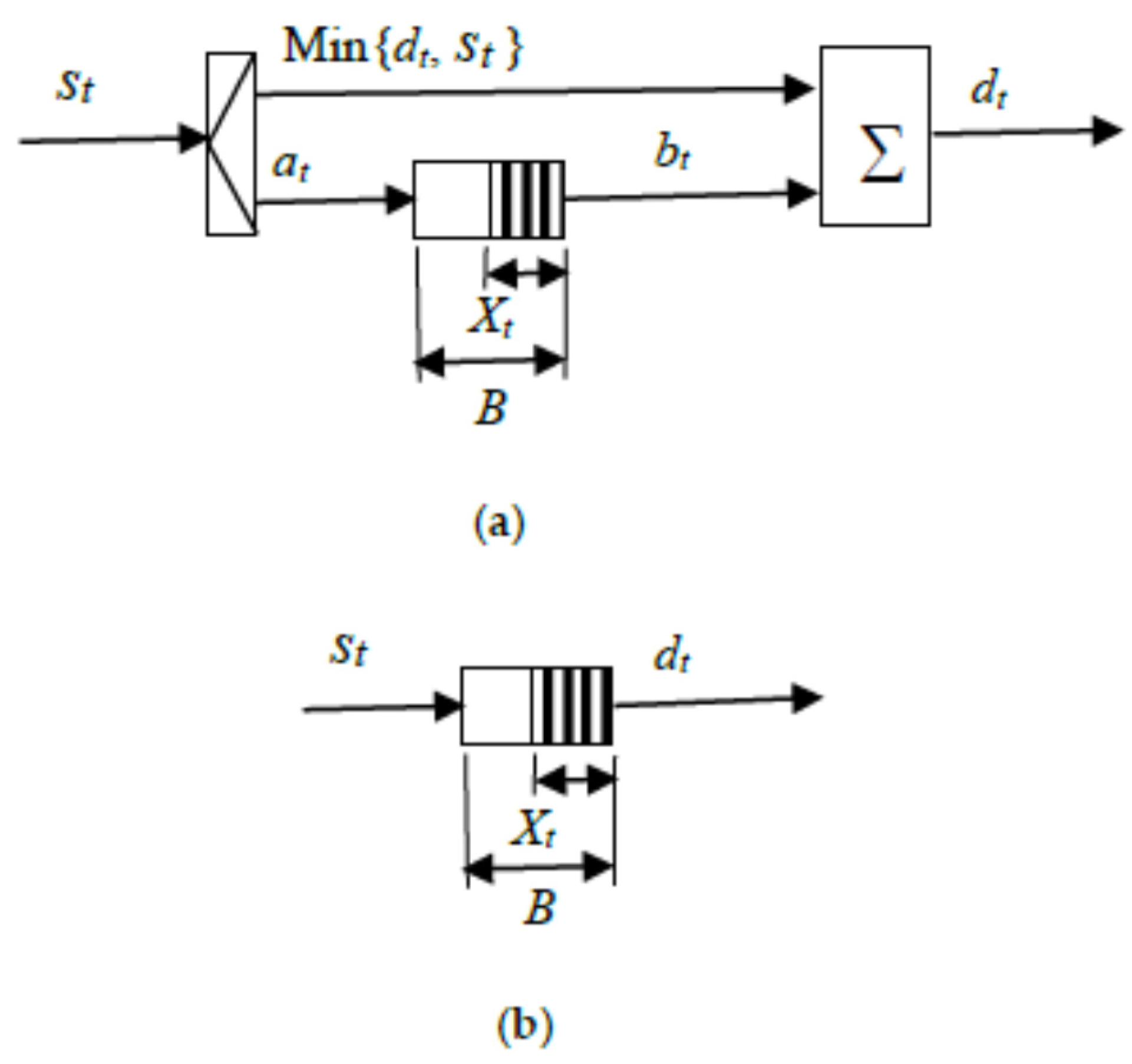
2. Fluid Approximation of Storage Systems

The fluid model of storage systems is a simple approximation of the complex operation of a storage device, which permits to obtain values for the main variables of design in less time than a simulation model. This method may be conveniently applied for storage sizing/analysis in wind/wave hybrid generation systems.

The modeling approach assumes that a set of n offshore generators generates a power s(t) and this power is transmitted to land by a cable line with finite capacity d(t). The corresponding energy terms at instant t = T are defined:

$$S_t={{\displaystyle \int }}_o^{T}s\left(t\right)dt{D}_t={{\displaystyle \int }}_o^{T}d\left(t\right)dt$$

(1)

When the generated renewable power is higher than the maximum capacity of the line, the excess of generated power:

a_t = max{0, (s_t − d_t)} = [s_t − d_t]⁺

(2)

is stored in a storage system. When generated power is less than the maximum power capacity of the line, the storage system supplies that power deficit:

b_t = [d_t − s_t]⁺

(3)

if it is possible, based on the storage state of charge. A_t and B_t are defined from a_t and b_t, similarly to S_t and D_t in Equation (1).

The storage process is modeled as a continuous stochastic process (Figure 1a). Let X_t be the state of charge of the storage system and X₀ its initial level, then

X_t = X₀ + A_t − B_t

(4)

Based on Equations (1)–(3), the storage process Equation (4) can be written as a function of S_t and D_t as follows:

X_t = X₀ + A_t − B_t = X₀ + S_t − D_t

(5)

Then, the state of charge can be written as a function of S_t and D_t, as shown in Figure 1b, that represents its equivalent storage system. Some of the non-ideal behaviors of the storage that were mentioned at the beginning of the section as storage charging and discharging rate limit, energy storage device efficiency, and depth of discharge can also be represented in the equivalent storage systems as explained in [35], and the capacity limit of the storage device will be explained in the next section.

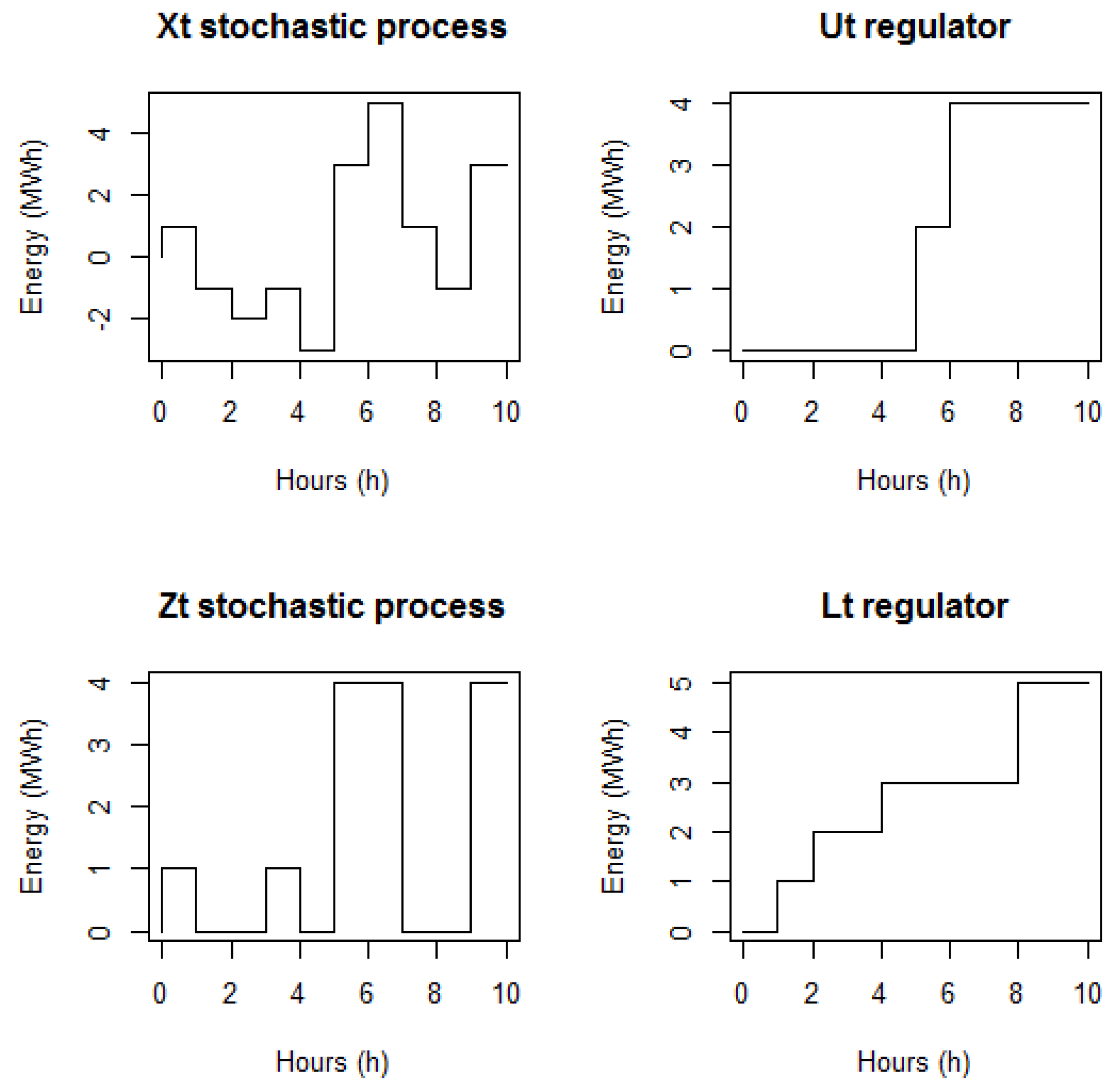
2.1. Regulated Brownian Model Approximation

In the previous section, the storage capacity was considered to be infinite, which is the ideal case. However, in real engineering applications, this storage capacity has a finite energy size, here called B. The processes L_t and U_t are defined, which are continuous and increasing with X₀ = 0. These processes are called regulators.

If the (expected) constant power delivery, d_t is higher than the generation and the storage is empty (X_t = 0), some power demand is not supplied. Let l_t be the demand not supplied at time t = T or loss of power, and the output of the storage system is b_t − l_t and the loss of energy L_t is,

$$L_t={{\displaystyle \int }}_0^T{l}_{t}dt$$

(6)

If the (expected) constant power delivery is less than the generation and the storage is full (X_t = B), some of the generated power is wasted. Let u_t be the waste of power at time t = T, then the input of the storage systems is a_t − u_t, and the waste of energy U_t is,

$$U_t={{\displaystyle \int }}_0^T{u}_{t}dt$$

(7)

Based on Equations (6) and (7), the storage process with finite storage capacity, Z_t, can be rewritten as:

Z_t = X₀ + (A_t − U_t) − (B_t − L_t) = X_t + L_t − U_t

(8)

For each trajectory defined by Z_t ∈ (0,B), there are an L_t and an U_t, and are unique: As can be seen in Figure 2, the U_t and L_t regulators control the Z_t process among 0 and B.

The control law used here is very simple. The storage system absorbs the difference between the generation and the demand until the storage is full, and it helps generators cover the power demand when the production from wind and wave resources is insufficient.

Hence, the calculation of L_t and U_t is made with these algorithms, implying the discretization of the time variable from t to k.

if ((X[k] + L[k − 1] − U[k − 1]) < lim_inf)
L[k] = L[k − 1] + (lim_inf − (X[k] + L[k − 1] − U[k − 1]))
else L[k] = L[k − 1]

if ((X[k] + L[k − 1] − U[k − 1]) > lim_sup)
U[k] = U[k − 1] + ((X[k] + L[k − 1] − U[k − 1]) − lim_sup)
else U[k] = U[k − 1]

where lim_inf and lim_sup are 0 and B, respectively.

It is possible to use other control strategies that could bring better performance, such as strategies with tunable parameters that can be optimized or optimal control, but the complexity of the analysis would be further increased, and thus only the basic control strategy is considered in this work.

2.2. Optimal Sizing of Storage System Modelled by Regulated Brownian Motion

The storage process described in Equation (8) is a regulated Brownian motion. The optimal control of this regulated Brownian motion [36] consists of designing a controller that monitors the content of the storage system and imposes a lower control barrier at zero and an upper control barrier at B. The control searches an optimal policy (L_t, U_t) which optimizes a profit function.

Storage system performance depends on its design characteristics and its operation, but these characteristics and operation have a cost. The profit function permits a tradeoff between performance and cost. The investment cost depends on the size of the storage, and the operation cost depends on: (i) the demand that cannot be met from system formed by the wind and wave generators plus storage, (i.e., loss of power, l_t), and that is lost with no adverse effect on future demand; and (ii) the generation excess that cannot be stored because the storage is full (i.e., waste of power, u_t).

The expected profit value is:

Expected profit = Income − Investment cost − Cost of waste and loss of energy

(9)

Following, the formulation of each term,

$$\text{Income}=E[p{\int }_0^{\infty }{e}^{-\mathsf{\lambda }t}dS]=\frac{p·\mathsf{\mu }}{\mathsf{\lambda }}$$

(10)

$$\text{Investment cost}=\text{Generation cost}+\text{Storage cost}=\frac{m·\max S}{pb}+\frac{h2·B}{pb}$$

(11)

$$\text{Cost of wasted and lost energy}=E[{\int }_0^{\infty }{e}^{-\mathsf{\lambda }t}\left(\mathsf{\alpha }dL+\mathsf{\beta }dU\right)]$$

(12)

where,

• E[], is the expected value of a stochastic variable.
• p, is the selling price of energy (€/kWh).
• S, is a stochastic variable with mean µ and standard deviation σ that represents the generated power (kW). Here, it is a normal distribution N (µ,σ).
• λ, is the interest rate.
• m, is the installation cost of (wind and wave) generators (€/kW).
• maxS, is the maximum power supplied by generators (kW).
• h2, is the installation cost of the storage system (€/kWh).
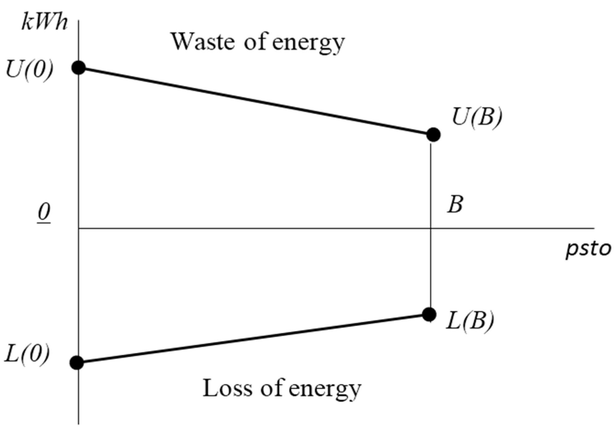
• B, is the energy capacity of the storage system (kWh).
• α, is the price of the loss of energy (€/kWh).
• β, is the price of the waste of energy (€/kWh).
• pb, payback time or number of years of amortization.

Equation (9) represents the profit of the generated energy, Equation (10) represents the ideal income, Equation (11) is the investment cost composed by generation cost plus storage cost, and Equation (12) is the total cost of wasted and lost energy, where αdL is the cost of the waste of power, and βdU is the cost of the loss of power. As the loss of power and the waste of power correspond to energy not sold, the constants α and β can be set equal to p.

These equations can be regrouped as:

$$k1=\frac{p·\mathsf{\mu }}{\mathsf{\lambda }}-\frac{m·\max S}{pb}-\frac{h2·B}{pb}$$

(13)

$$k2\left(x\right)=E\left[{{\displaystyle \int }}_0^{\infty }{e}^{-\lambda t}\left(\mathsf{\alpha }dL+\mathsf{\beta }dU\right)\right]$$

(14)

The term k2(x) is the Ito’s integral of a stochastic process and the solution is Equation (15). The variable x is the starting state of Brownian motion. A mathematical proof of these results is in [36].

$$k2\left(x\right)=\{\begin{array}{c}-\beta \frac{g\left(x\right)}{g^{\prime }\left(b\right)}+\mathsf{\alpha }\frac{g\left(x-b\right)}{g^{\prime }\left(-b\right)},0\le x\le b\\ k2\left(x\right)=k2\left(b\right)+\left(x-b\right)r,x>b\end{array}$$

(15)

where, g(x) is a bounded family of random variables. To a Brownian motion N(µ,σ), the two values $a^{*}\left(\mathsf{\lambda }\right)$ and $a_{*}\left(\mathsf{\lambda }\right)$ are roots of $\mathsf{\mu }a+\frac{{\mathsf{\sigma }}^2}{2}{a}^2=\mathsf{\lambda }$, substituting a = $a^{*}\left(\mathsf{\lambda }\right)$ and a = −$a_{*}\left(\mathsf{\lambda }\right)$.

$$g\left(x\right)=a_{*}\left(\mathsf{\lambda }\right)\exp \left(a^{*}\left(\mathsf{\lambda }\right)x\right)+a^{*}\left(\mathsf{\lambda }\right)\exp \left(-a_{*}\left(\mathsf{\lambda }\right)x\right)$$

(16)

where

$$a_{*}=\frac{\mathsf{\mu }+\sqrt{{\mathsf{\mu }}^2+2{\sigma }^2\mathsf{\lambda }}}{{\mathsf{\sigma }}^2}\text{ and }{a}^{*}=\frac{-\mathsf{\mu }+\sqrt{{\mathsf{\mu }}^2+2{\mathsf{\sigma }}^2\mathsf{\lambda }}}{{\mathsf{\sigma }}^2}$$

(17)

2.3. Optimal Converter Power Rating for the Storage System Modelled by Brownian Motion

In the above section, the optimal control does not depend on the rating of the power electronics converter associated to the storage, it only depends on the energy capacity, B, of the storage. The finite power rating of the converter, psto, limits the power input a_t to the storage system, as well as the power output, b_t, thus defining the actual power capability of the storage system. Here, this aspect is modeled with the installation cost of the power converter and attenuation parameter of the waste and loss of power.

$$converterpowercost=\frac{h3·psto}{pb}$$

(18)

where, h3 is the price for converter power unit.

If the power converter capability is B divided by time unit, the waste and loss of energy are calculated as in Section 2.1. If the power converter rating is zero, the waste and loss of power are the same that if the energy capacity of the storage was zero. Between these two cases, a linear approximation is made as it shows Figure 3.

$$\left(psto\right)=\frac{U\left(B\right)-U\left(0\right)}{B}·psto+U\left(0\right)$$

(19)

$$L\left(psto\right)=\frac{L\left(B\right)-L\left(0\right)}{B}·psto+L\left(0\right)$$

3. Wind and Wave Generators Models

In the most simplified approximation, models used for wind and wave energy converters can be based on power curves of the generators that allow converting resource data into extracted power. Then, the total power generated by wave-wind farm can be obtained with a combination of the power generated by each device.

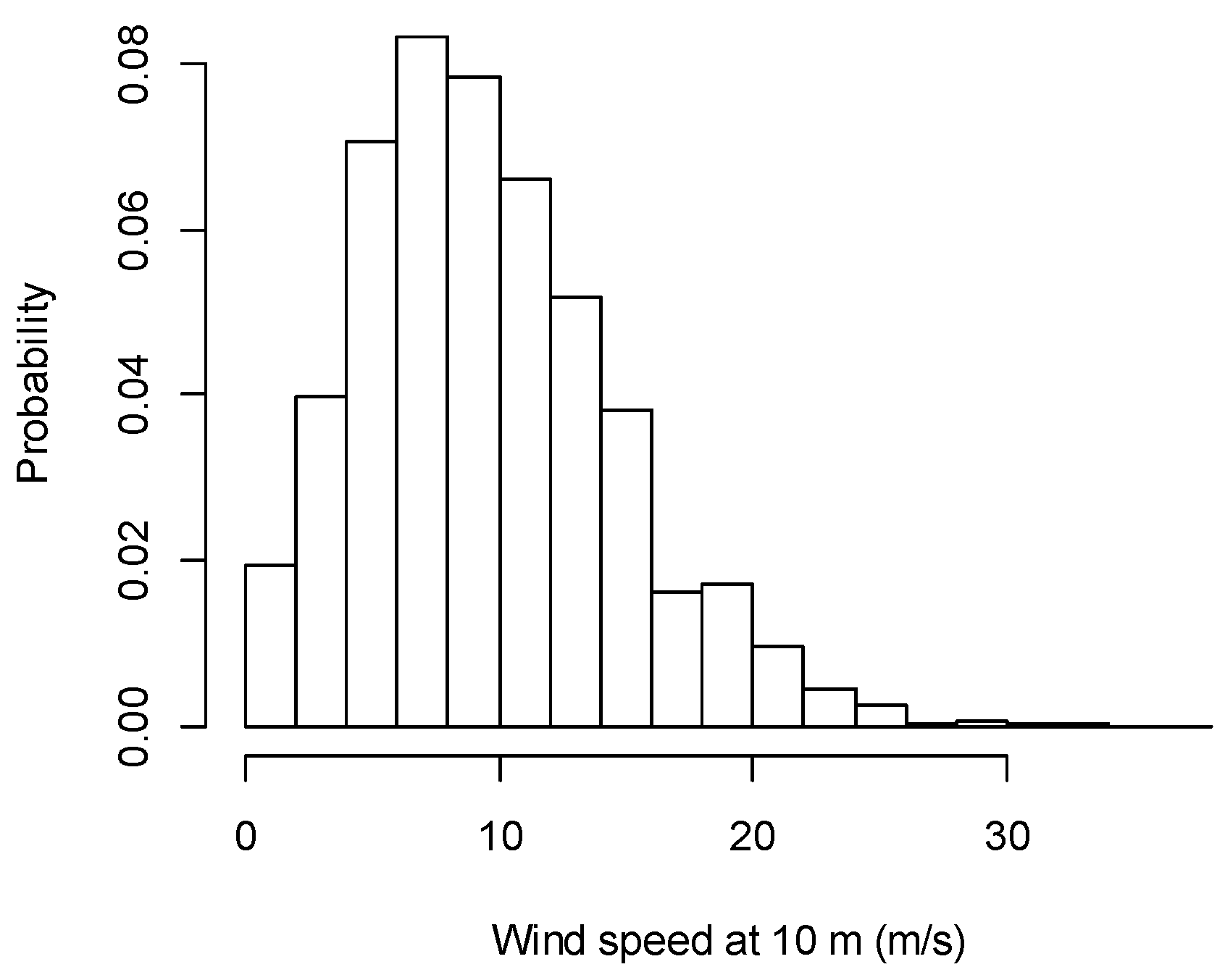
3.1. Wind Generator Model

The average power output of the wind generator in the time interval of 3 h is calculated from its speed-power curve defined as [37],

$${\mathsf{\omega }}_s\left(t\right)={\mathsf{\omega }}_{s0}\left(\mathrm{t}\right)·{\left(\frac{z_r}{z}\right)}^{0.143}$$

(20)

$$P_w\left(t\right)=\{\begin{array}{c}0if{\mathsf{\omega }}_s\left(\mathrm{t}\right)<4m/s\\ P_N{\left(\frac{{\mathsf{\omega }}_s\left(\mathrm{t}\right)}{{\mathsf{\omega }}_N}\right)}^{3}if4\le {\mathsf{\omega }}_s\left(\mathrm{t}\right)\le 11m/s\\ P_{N}if11\le {\mathsf{\omega }}_s\left(\mathrm{t}\right)\le 25m/s\\ 0if{\mathsf{\omega }}_s\left(\mathrm{t}\right)>25m/s\end{array}$$

(21)

where, ω_s is the wind speed at the height of the turbine (m/s), z_r is the height of the turbine, z is the height of the measure tower, ω_s0 is the speed at the height z, ω_N is the rated wind speed and P_N the rated turbine power.

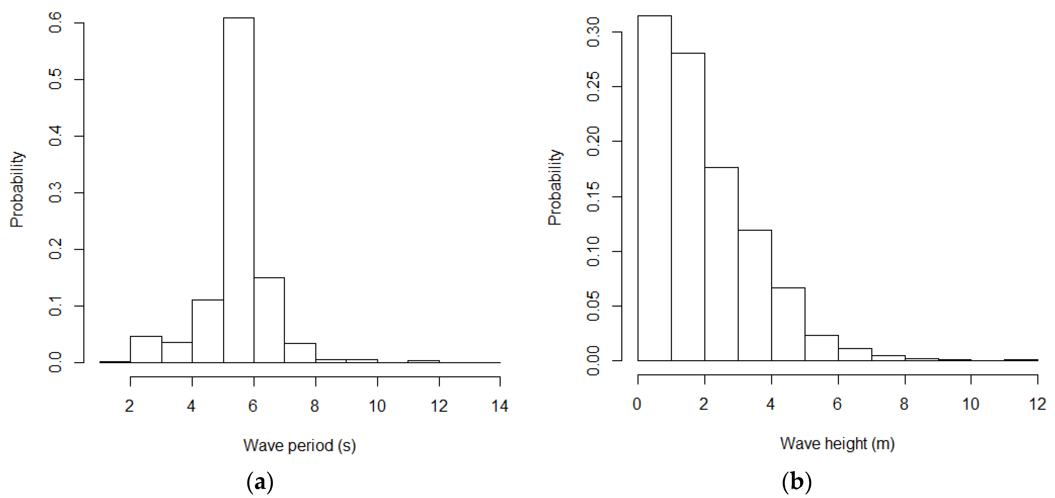
3.2. Wave Generator Model

The power output of the wave generator is calculated considering heaving buoys as target devices and representing their power extraction capability by a simplified filtering approach [38], as follows:

$$P_{wv}\left(t\right)=\frac{\rho g^2}{64\pi }·H_{m0}^2\left(\mathrm{t}\right)·T_e\left(\mathrm{t}\right)·PTF\left(\mathrm{t}\right)·d_w$$

(22)

$$P_{wv}\left(t\right)=\frac{\rho g^2}{64\pi }·H_{m0}^2\left(\mathrm{t}\right)·T_e\left(\mathrm{t}\right)·PTF\left(\mathrm{t}\right)·d_w$$

(23)

where, P_wv is the average wave extracted power calculated in our case over the time interval of 3 h, H_m0 is the significant wave height, T_e is the wave energy period, ρ is the water density, g the acceleration of gravity and d_w is the diameter of the wave device. PTF is the gain of the transfer function of the buoy power, evaluated at f = 1/T_e, with the parameters: a_w attenuation factor, f_c central tuning frequency of the control system, and f the inverse of T_e and σ_w the width of the transfer function.

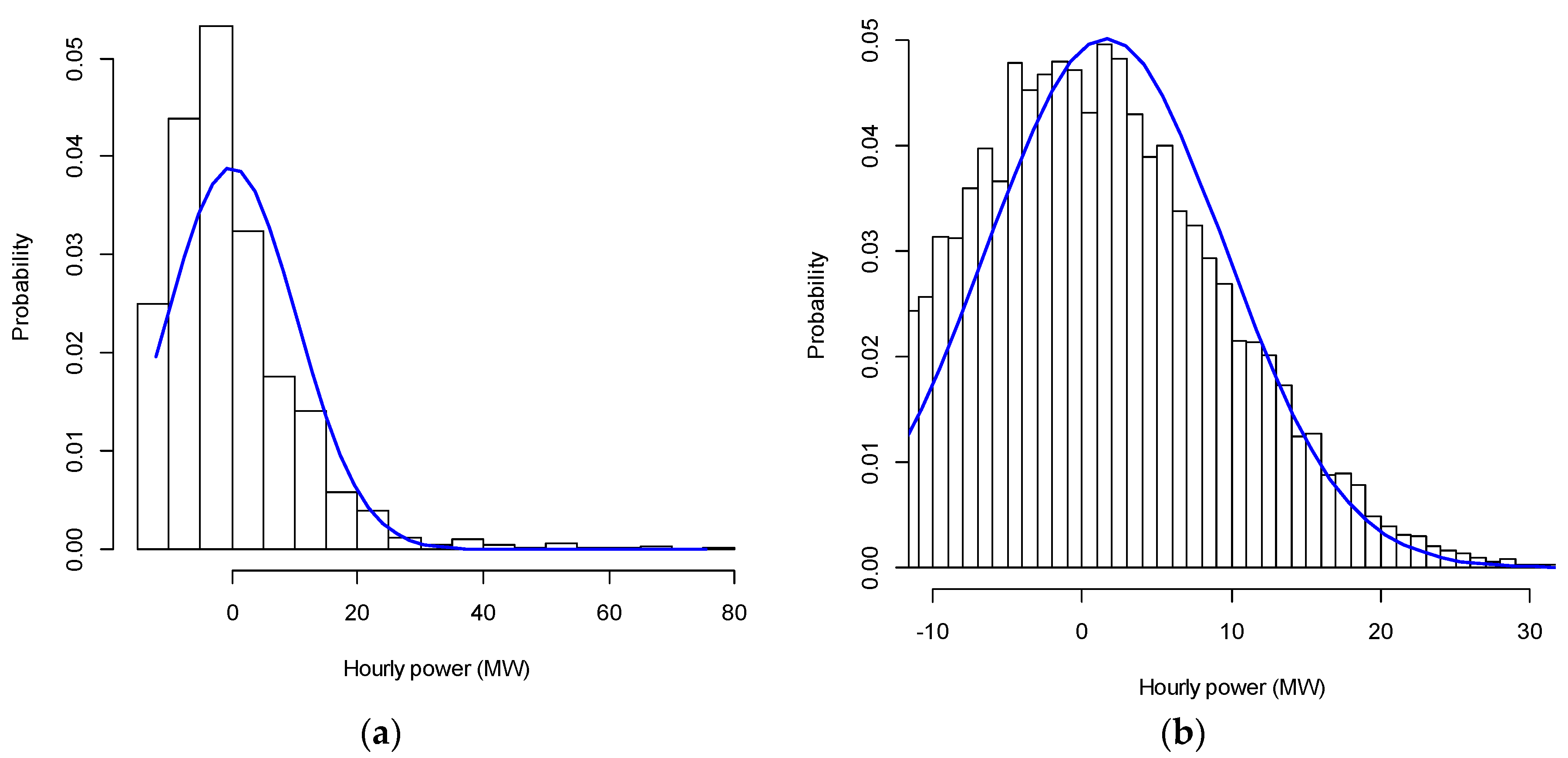
3.3. Aggregate Power Output from the Wind–Wave Farm

The generated power of every device (wind or wave generator) depends on variables that are functions of time, the speed ω_s0(t) for the wind generator and H_m0(t), T_e(t), and f(t) for wave generator. There is generally a time series of each variable for a site, but it is possible to generate a correlated time series v_new(t) from the original series v₀(t) for each device adding a Gaussian noise centered in zero ε(t).

$$v_{new}\left(t\right)=v_0\left(t\right)+\mathsf{\epsilon }\left(t\right)$$

(24)

The offshore wind farms have wave losses estimated between 0.06 and 0.2 p.u. of total power, reducing the efficiency to between 0.8 and 1 p.u., and the wave farms have a similar wave loss effect that reduces the efficiency between 0.5 and 1 p.u. Then, the aggregate power output of the wind–wave farm is calculated from,

$$P_{farm}\left(t\right)={\mathsf{\eta }}_w{\displaystyle \sum }_{i=1}^{n_w}{P}_{w,i}\left(t\right)+{\mathsf{\eta }}_{wv}{\displaystyle \sum }_{j=1}^{n_{wv}}{P}_{wv,j}\left(t\right)$$

(25)

where

• ${\eta }_w$, is the wind farm efficiency.
• $n_w$, is the number of wind generators.
• ${\eta }_{wv}$, is the wave farm efficiency.
• $n_{wv}$, is the number of wave generators.

4. Genetic Algorithm

The optimization problem can be written as a maximization algorithm, i.e.,

Max: Profit(B, psto)
Subject to: B > 0, psto > 0

(26)

Several optimization algorithms can solve this problem. In this work, Genetic algorithms with real valued function [39] are chosen, which are stochastic search algorithms based on the mechanisms of the natural evolution: selection, crossover and mutation. The fittest individuals dominate over the weaker ones, mimicking the biological evolution.

5. Simulation Results

5.1. Description of Input Data

In order to test the considered energy storage sizing methodology in a realistic scenario, real wind and wave meteorological data from the British Atmospheric Data Centre’s MIDAS marine surface measurements [40] were used. The chosen site is Sedco 711 in the Irish Sea with data from 2007 to 2011 and with time resolution of 3 h. The location is close enough to potential round three offshore wind sites in UK waters. The elaboration of these data provides the probabilistic distribution functions (pdf) of the wind speed, significant wave height and wave period, which are represented by histograms in Figure 4 and Figure 5.

From the application of Equations (20)–(25), the time evolution of the power extraction is calculated from a hybrid farm, designed to give a 50%–50% of average wind/wave power share, and assuming: z_r = 70 m, ω_n = 11.6 m/s, P_N = 1.5 MW, ρ = 1025 kg/m3, g = 9.8 m/s2, d_w = 20 m, a_w = 0.4, f_c = 0.179 Hz, and σ_w = 0.025.

The wind-wave farm is formed by 6 wind generators of 1.6 MW-peak and 138 buoys of 345 kW-peak.

Then, the probabilistic distribution functions of the output power from the wind-wave farm of 57.2 MW of installed power (and 12 MW of average power) is calculated and shown in Figure 6 for a wind and wave efficiency of 0.9, and a Normalized Gaussian noise (m = 0, sd = 0.2). The difference between the power generation and the cable limit capacity (which is set to d = 12 MW) gives the probabilistic distribution function to be used as an input to the storage device, shown in Figure 7. In Figure 7b, it can be seen that the difference between the probabilistic distribution functions of the generation does not correspond to a simple translation of load, i.e., Figure 7b does not correspond to a simple translation of Figure 6b. This function is truncated symmetrically at both sides of zero by the power of the power electronics interface, psto, of the storage device. As a final step, this truncated function is approximated by a normal function. This is because the fluid model used here assumes inputs with normal distributions although the real data may not have a normal distribution. The normal distribution approximation is anyway conservative, because the states with deficit of power in the extraction line have greater probability than the symmetrical states with excess of power.

Equation (17) uses the standard deviation of the storage process. If the storage design is aimed at ensuring the energy supply over an hour, it is necessary to introduce the hourly variability, while, if the design aims at ensuring the supply over a week, it is necessary to introduce the weekly variability. Probabilistic distribution functions must reflect the variability over the time interval desired, because the greater the time interval is, the greater the variability is. The evolution of the power variability is shown in Figure 8 from a 3 h data to a one-week data. The longer the time interval considered, the more the standard deviation of the power decreases, the mean is similar and the distribution function approaches the Gaussian distribution. The evolution of the energy variability is shown in Figure 9 from 3-h data to one-week data. Here, the standard deviation and the mean increase with the time interval, and the distribution function approaches the Gaussian distribution. The performance of the power influences the size of the converter and the performance of the energy influences the size of the storage device.

Considered economic data in this test case are the following. Energy price is 300 €/MWh, the effective holding cost (h) is zero, time horizon (T) is 8760 h, initial state of storage (X₀) is zero, the costs of wasted power (α) and lost power (β) are both 300 €/MWh, the installation cost of wind power is 1000 €/MW, the installation cost of wave power is 2000 €/MW, the installation cost of storage energy [41] is 300 €/kWh, the installation cost of storage converter [42] is 80 €/kW, and payback time is 10 years, interest rate per year (λ) is 5%.

The parameters used in the genetic algorithm are population size 100 individuals and the number of generations (number of iterations) 1000. The fitness function is the Expected profit defined in Equation (9). The chosen values for probability of crossover and mutation are 0.8 and 0.1, respectively.

In this paper, we have compared the fluid model with two simulation models: Monte Carlo simulation with real data and Monte Carlo simulation with input data approximated by a normal distribution. In Figure 10, the comparison of both types of inputs can be seen.

5.2. Studied Cases

The studied cases are:

Case 1:

Monte Carlo simulation of hybrid wave-wind generation system without storage and real data.

Case 2:

Monte Carlo simulation of hybrid wave-wind generation system without storage and approximated data.

Case 3:

Fluid model of hybrid wave-wind generation system without storage.

Case 4:

Optimal sizing of storage system with the Monte Carlo simulation and real data.

Case 5:

Optimal sizing of storage system with the Monte Carlo simulation and approximated data.

Case 6:

Optimal sizing of storage system with the fluid model.

The first three cases are the results of the models without storage, and the last three cases are the results obtained to optimize the storage size with the different models. The simulations use successive values from the real time series in Cases 1 and 4, while they use independent sampling from PDF distributions in Cases 2 and 5.

Main results are shown in

Table 1. Summary of results in a year for different cases.

	Case 1	Case 2	Case 3	Case 4	Case 5	Case 6
B (MWh)	–	–	–	37.23	87.46	62.09
psto (MW)	–	–	–	9.43	22.82	15.09
Convergence time of the algorithm	–	–	–	5.84 min	2.48 min	5.71 s
Produced energy (GWh)	105.12	105.12	105.12	105.12	105.12	105.12
Waste of energy (GWh)	32.42	31.64	35.80	26.48	3.38	2.87
Loss of energy (GWh)	32.42	31.64	35.81	26.49	3.42	2.90
Extracted energy (GWh)	72.70	73.48	69.31	78.63	101.70	102.22
Wasted energy cost (%)	31.72	30.96	35.03	25.91	3.31	2.81
Lost energy cost (%)	31.72	30.96	35.03	25.91	3.34	2.84
Income (%)	71.12	71.88	67.81	76.93	99.50	100.00
Investment (%)	–	–	–	3.89	9.15	6.47
Profit (%)	71.12	71.88	67.81	73.04	90.34	93.53
Capacity factor	0.691	0.698	0.659	0.748	0.967	0.972

. All cases have the same produced energy, the same mean and the same standard deviation to facilitate the comparison. Although the models produce the same energy, the waste and loss of energy are different because the distributions are different. Extracted energy is the energy transported by the transmission line to land, and is equal to produced energy minus loss of power along the year. The investment is the annual cost of the storage system with a payback time of ten years.

All the cost items are normalized over the maximum value of income, resulting from the six cases, i.e., 30.66 M€.

With the storage installation, all models increase the profit as well as the capacity factor of the line. The utilization of storage permits to use at its maximum capacity almost all the time. This capacity factor without storage is estimated to be between 65.9% and 69.8%. With storage deployment, it is bigger in Cases 5 (96.7%) and 6 (97.2%) than in Case 4 (74.8%) because the installed storage is bigger. The approximated models attain better results than the real case, however they significantly overestimate the real results and oversize the storage system because they do not reproduce the effect of temporal structure as it can be seen in Cases 5 and 6. Fluid model is significantly faster than Monte Carlo simulations.

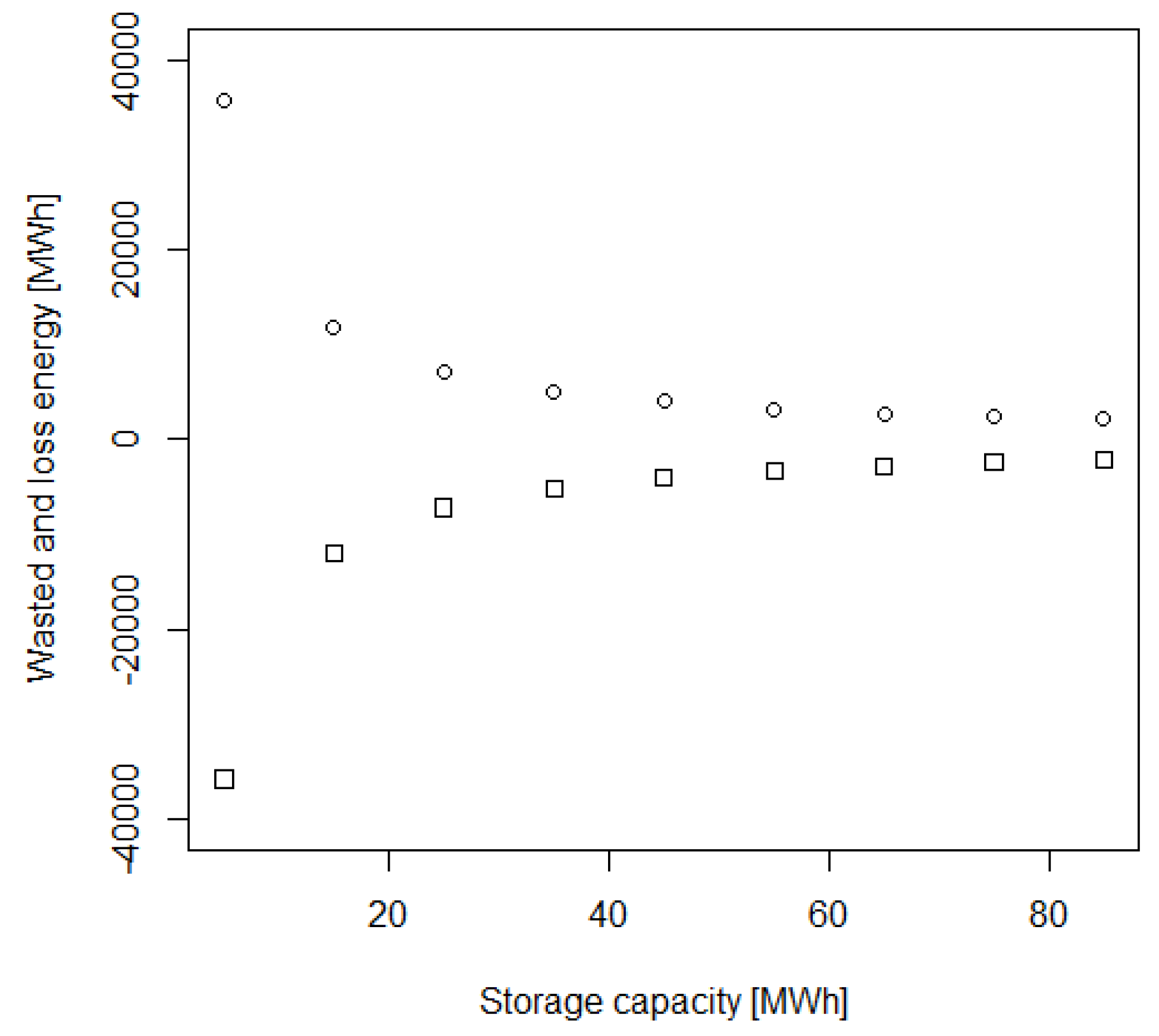
5.3. Sensitivity of the Wasted and Loss Energy to the Storage Sizing

In Figure 11, it is possible to see the dependency of the wasted and lost energy on the storage capacity in the fluid model. The optimal size chosen in Case 6, 62.09 MWh, coincides with the point of smallest capacity where the wasted and loss energy are stabilized. By further increasing the storage capacity installed, there is a negligible decrease in wasted and lost energy for the same storage capacity increment.

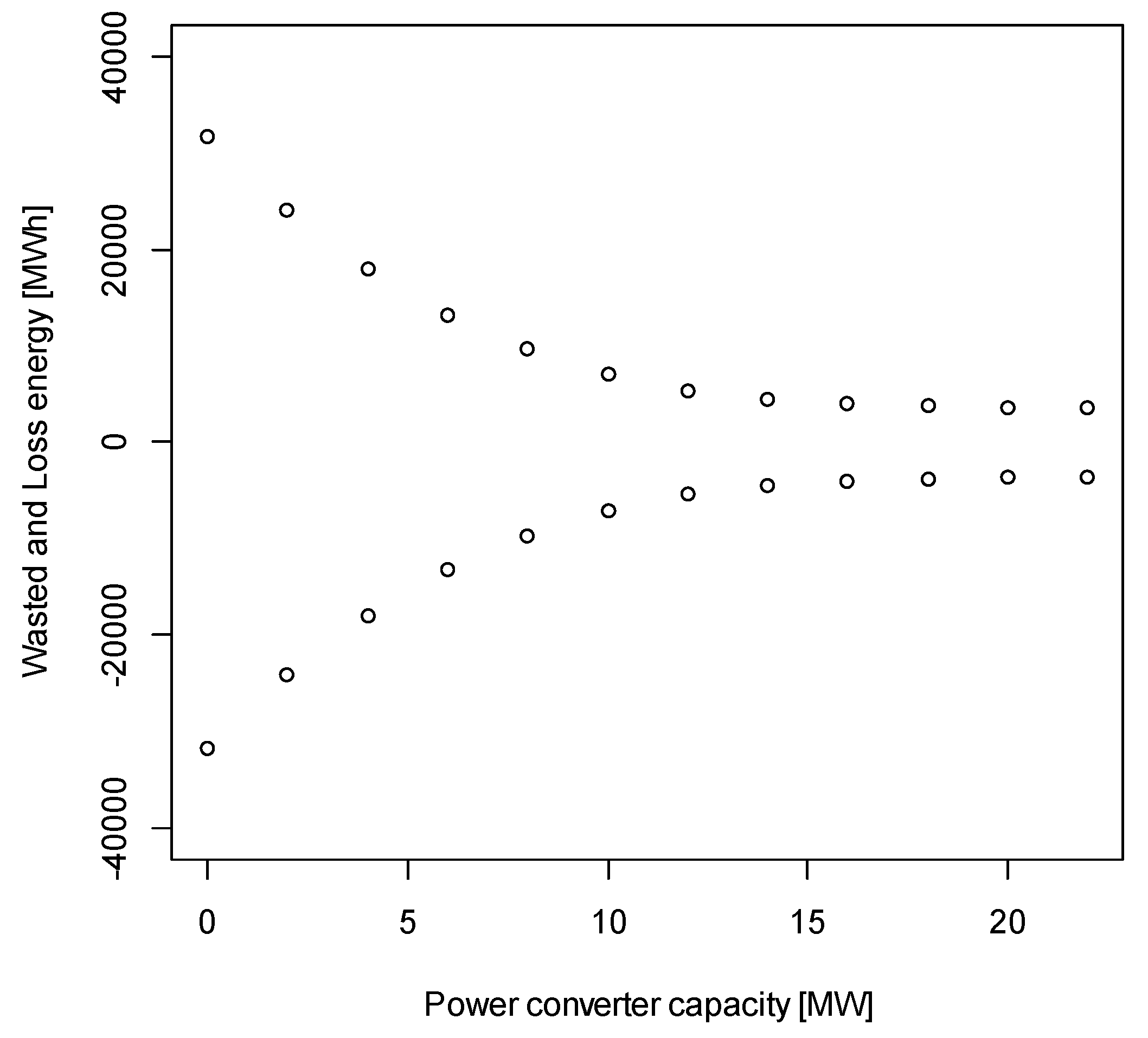
5.4. Sensitivity of the Wasted and Lost Energy to the Converter Power Rating

The wasted and lost energy also depends of the power converter rating. The evolution of wasted and lost energy is shown in Figure 12. When the power converter capacity is zero, the wasted and loss energy is maximum (31.64 GWh) and when the power converter capacity is high (22.82 kW), the wasted and loss energy is minimum (3.4 GWh). These values match with the values of Case 2 and 5.

There is a difference between the real values and the linear approximation presented in Section 2.2, but the approximation is conservative, because the wasted and lost energy is bigger in the approximation model than in the real model.

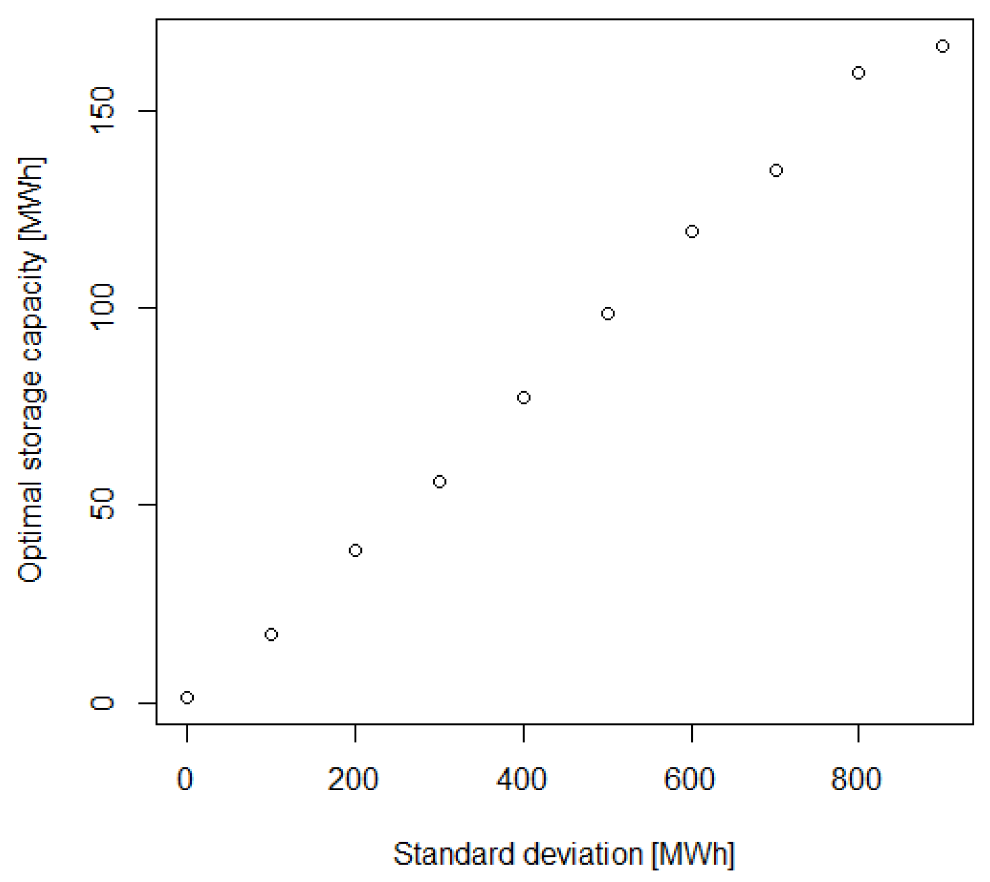
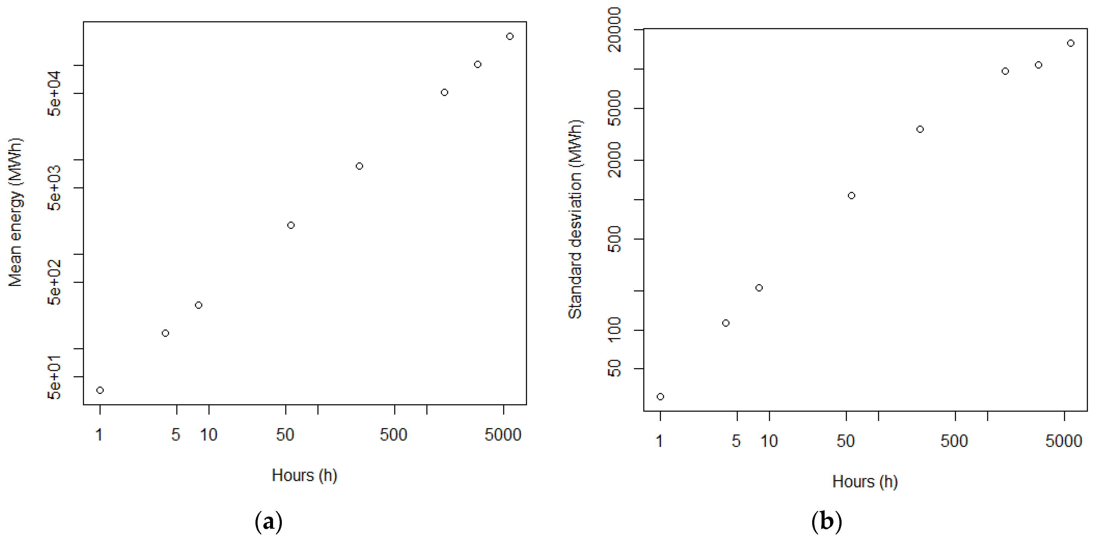
5.5. Sensitivity of the Storage Sizing to the Variability of the Input Power

Storage systems must compensate the variability of the energy flow from the wind/wave energy farm. For the same flow, this variability depends on the considered time interval, in which the compensation is implemented. In Figure 13, the variability of power input in several time intervals (1 h, 12 h, 24 h, one week, one month, six months, one year, and two years), which is measured with the standard deviation, is shown.

The optimal (energy) storage capacity (B) needed to compensate the variability according to the fluid method developed in this paper is shown in Figure 14 as a function of the energy standard deviation.

6. Conclusions

In this paper, the potential use of a fluid model for sizing the energy storage systems in a hybrid wave-wind generation farm has been investigated. Fluid models have recently raised interest and been increasingly used in the design of storage systems for renewable energy applications because of the ease of implementation and much higher time-effectiveness than traditional simulation models.

Although the investigation performed has confirmed that fluid models have a convergence time that is in the order of 30–60 times lower than a corresponding Monte Carlo simulation, the resulting storage sizing results in a significant oversizing of the storage device (66% in terms of energy and 60% in terms of power), compared to a Monte Carlo simulation based on real data.

One reason for this lies in the fact that the fluid model relies on the use of a normal distribution of the input data and therefore, the quality of the final result depends on how well such normal distribution resembles the characteristics of the real input data for the considered application. It should be noted that the use of simplified model to derive the power extraction of wind turbines and wave energy converters may have an impact on the considered distributions, which could be evaluated more in detail only through the availability of real power curves of such devices. Anyway, for the considered test case, the assumption of normal distribution of the input generated power seems not to be valid at a satisfactory extent.

Comparison of the results obtained from the fluid model and a corresponding Monte Carlo simulation, both run starting from the same approximated input data (i.e., data presenting a normal distribution) has shown that the fluid model provides a solution whose size is only 66%–70% of that of the corresponding extensive simulation model, with a profit reduction of only about 5%.

Based on the previous considerations, the fluid model, in its current formulation, looks applicable only as a preliminary design tool for the design of energy storage installations in hybrid wave-wind energy farms, while more specific simulation studies will still be required for the final design. Refined fluid models could be also elaborated and tested, which can possibly be less sensitive to the deviation of real input data from the normal distribution.

Anyway, the six test cases considered over a one-year period have also proved that, under the specified techno-economic assumptions, the deployment of an energy storage system capable of reducing the variability of the generated power and hence increasing the capacity factor of the electric infrastructure, can be profitable for hybrid wind-wave energy farms of medium size.

References

1. Pérez-Collazo, C.; Greaves, D.; Iglesias, G. A review of combined wave and offshore wind energy. Renew. Sustain. Energy Rev. 2015, 42, 141–153. [Google Scholar] [CrossRef]
2. The European Wind Energy Association. The European offshore wind industry—key trends and statistics 2014. Available online: http://www.ewea.org/fileadmin/files/library/publications/statistics/EWEA-European-Offshore-Statistics-2014.pdf (accessed on 29 February 2016).
3. Widén, J.; Carpman, N.; Castellucci, V.; Lingfors, D.; Olauson, J.; Remouit, F.; Bergkvist, M.; Grabbe, M.; Waters, R. Variability assessment and forecasting of renewables: A review for solar, wind, wave and tidal resources. Renew. Sustain. Energy Rev. 2015, 44, 356–375. [Google Scholar] [CrossRef]
4. Stoutenburg, E.D.; Jenkins, N.; Jacobson, M.Z. Power output variations of co-located offshore wind turbines and wave energy converters in California. Renew. Energy 2010, 35, 2781–2791. [Google Scholar] [CrossRef]
5. Soukissian, T.H. Probabilistic modeling of directional and linear characteristics of wind and sea states. Ocean Eng. 2014, 91, 91–110. [Google Scholar] [CrossRef]
6. Güner, H.A.A.; Yüksel, Y.; Çevik, E.Ö. Estimation of wave parameters based on nearshore wind-wave correlations. Ocean Eng. 2013, 63, 52–62. [Google Scholar] [CrossRef]
7. Fusco, F.; Nolan, G.; Ringwood, J.V. Variability reduction through optimal combination of wind/wave resources—An Irish case study. Energy 2010, 35, 314–325. [Google Scholar] [CrossRef]
8. Tedeschi, E.; Robles, E.; Santos, M.; Duperray, O.; Salcedo, F. Effect of energy storage on a combined wind and wave energy farm. In Proceedings of the Energy Conversion Congress and Exposition, Raleigh, NC, USA, 15–20 September 2012; pp. 2798–2804.
9. Astariz, S.; Perez-Collazo, C.; Abanades, J.; Iglesias, G. Towards the optimal design of a co-located wind–wave farm. Energy 2015, 84, 15–24. [Google Scholar] [CrossRef]
10. Chozas, J.F.; Kramer, M.M.; Sørensen, H.C.; Kofoed, J.P. Combined Production of a Full-scale Wave Converter and a Full-scale Wind Turbine—A Real Case Study. Int. Conf. Ocean Energy 2012, 2012, 1–7. [Google Scholar]
11. Hanssen, J.E.; Margheritini, L.; O’Sullivan, K.; Mayorga, P.; Martinez, I.; Arriaga, A.; Agos, I.; Steynor, J.; Ingram, D.; Hezari, R.; et al. Design and performance validation of a hybrid offshore renewable energy platform. In Proceedings of the 2015 10th International Conference on Ecological Vehicles and Renewable Energies, Monte-Carlo, Monaco, 31 March–2 April 2015; pp. 1–8.
12. Zhou, Z.; Benbouzid, M.; Charpentier, J.F.; Scuiller, F.; Tang, T. A review of energy storage technologies for marine current energy systems. Renew. Sustain. Energy Rev. 2013, 18, 390–400. [Google Scholar] [CrossRef] [Green Version]
13. Slocum, A.H. Symbiotic offshore energy harvesting and storage systems. Sustain. Energy Technol. Assess. 2014. [Google Scholar] [CrossRef]
14. Aubry, J.; Bydlowski, P.; Multon, B.; Ahmed, H.B.; Borgarino, B. Energy Storage System Sizing for Smoothing Power Generation of Direct Wave Energy Converters. In Proceedings of the 3rd International Conference on Ocean Energy, Bilbao, Spain, 6–8 October 2010; pp. 1–7.
15. O’Sullivan, D.; Murray, D.; Hayes, J.; Egan, M.G.; Lewis, A.W. The Benefits of Device Level Short Term Energy Storage in Ocean Wave Energy Converters. In Energy Storage in the Emerging Era of Smart Grids; Carbone, R., Ed.; InTech: Rijeka, Croatia, 2011; Available online: http://www.intechopen.com/books/energy-storage-in-the-emerging-era-of-smart-grids/the-benefits-of-device-level-short-term-energy-storage-in-ocean-wave-energy-converters (accessed on 29 February 2016).
16. Tedeschi, E.; Santos-Mugica, M. Modeling and Control of a Wave Energy Farm Including Energy Storage for Power Quality Enhancement: The Bimep Case Study. IEEE Trans. Power Syst. 2014, 29, 1489–1497. [Google Scholar] [CrossRef]
17. Kovaltchouk, T.; Blavette, A.; Ahmed, H.B.; Multon, B.; Aubry, J. Comparison between centralized and decentralized storage energy management for Direct Wave Energy Converter Farm. In Proceedings of the IEEE 10th International Conference on Ecological Vehicles and Renewable Energies, Monte-Carlo, Monaco, 31 March–2 April 2015.
18. Marañon-Ledesma, H.; Tedeschi, E. Energy Storage Sizing by Stochastic Optimization for a combined Wind–wave-Diesel Supplied System. In Proceedings of the IEEE 4th International Conference on Renewable Energies and Applications, Palermo, Italy, 22–25 November 2015.
19. Tedeschi, E.; Sjolte, J.; Molinas, M.; Santos, M. Stochastic rating of storage systems in isolated networks with increasing wave energy penetration. Energies 2013, 6, 2481–2500. [Google Scholar] [CrossRef] [Green Version]
20. Rabiee, A.; Khorramdel, H.; Aghaei, J. A review of energy storage systems in microgrids with wind turbines. Renew. Sustain. Energy Rev. 2013, 18, 316–326. [Google Scholar] [CrossRef]
21. Oudalov, A.; Cherkaoui, R.; Beguin, A. Sizing and optimal operation of battery energy storage system for peak shaving application. In Proceedings of the IEEE Lausanne Power Tech, Lausanne, Switzerland, 1–5 July 2007; pp. 621–625.
22. Nick, M.; Cherkaoui, R.; Paolone, M. Optimal siting and sizing of distributed energy storage systems via alternating direction method of multipliers. Int. J. Electr. Power Energy Syst. 2015, 72, 33–39. [Google Scholar] [CrossRef]
23. Chen, S.X.; Gooi, H.B.; Wang, M.Q. Sizing of energy storage for microgrids. IEEE Trans. Smart Grid 2012, 3, 142–151. [Google Scholar] [CrossRef]
24. Barton, J.P.; Infield, D.G. A probabilistic method for calculating the usefulness of a store with finite energy capacity for smoothing electricity generation from wind and solar power. J. Power Sources 2006, 162, 943–948. [Google Scholar] [CrossRef]
25. Bludszuweit, H.; Dominguez-Navarro, J.A. A Probabilistic Method for Energy Storage Sizing Based on Wind Power Forecast Uncertainty. IEEE Trans. Power Syst. 2011, 26, 1651–1658. [Google Scholar] [CrossRef]
26. Song, J.; Krishnamurthy, V.; Kwasinski, A.; Sharma, R. Development of a markov-chain-based energy storage model for power supply availability assessment of photovoltaic generation plants. IEEE Trans. Sustain. Energy 2013, 4, 491–500. [Google Scholar] [CrossRef]
27. Jones, G.L.; Harrison, P.G.; Harder, U.; Field, T. Fluid queue models of renewable energy storage. In Proceedings of the 6th International Conference on Performance Evaluation Methodologies and Tools, Cargese, France, 9–12 October 2012; pp. 224–225.
28. Ghiassi-Farrokhfal, Y.; Keshav, S.; Rosenberg, C. Toward a Realistic Performance Analysis of Storage Systems in Smart Grids. IEEE Trans. Smart Grid 2015, 6, 402–410. [Google Scholar] [CrossRef]
29. Wang, K.; Member, S.; Ciucu, F.; Lin, C.; Member, S.; Low, S.H. A Stochastic Power Network Calculus for Integrating Renewable Energy Sources into the Power Grid. IEEE J. Sel. Areas Commun. 2012, 30, 1037–1048. [Google Scholar] [CrossRef]
30. Gautam, N.; Xu, Y.; Bradley, J.T. Meeting inelastic demand in systems with storage and renewable sources. In Proceedings of the IEEE International Conference on Smart Grid Communications, Venice, Italy, 3–6 November 2014.
31. Yan, K. Fluid Models for Production-Inventory Systems. Ph.D. Dissertation, The University of North Carolina at Chapel Hill, Chapel Hill, NC, USA, 2006. Available online: http://www.unc.edu/~vkulkarn/PhD/YanDissertation.pdf (accessed on 29 February 2016). [Google Scholar]
32. Aggarwal, V.; Gautam, N.; Kumara, S.R.T.; Greaves, M. Stochastic fluid flow models for determining optimal switching thresholds. Perform. Eval. 2005, 59, 19–46. [Google Scholar] [CrossRef]
33. Jones, G.L.; Harrison, P.G.; Harder, U.; Field, T. Fluid queue models of battery life. In Proceedings of the 2012 IEEE 20th International Symposium on Modeling, Analysis and Simulation of Computer and Telecommunication Systems, Arlington, VA, USA, 7–9 August 2012; pp. 278–285.
34. Mohammadi, S.; Mohammadi, A. Stochastic scenario-based model and investigating size of battery energy storage and thermal energy storage for micro-grid. Int. J. Electr. Power Energy Syst. 2014, 61, 531–546. [Google Scholar] [CrossRef]
35. Ardakanian, O.; Keshav, S.; Rosenberg, C. On the use of teletraffic theory in power distribution systems. In e-Energy’12, Proceedings of the 3rd International Conference on Future Energy System: Where Energy, Computing and Communication Meet, Madrid, Spain, 9–11 May 2012; ACM: New York, NY, USA, 2012. [Google Scholar] [CrossRef]
36. Harrison, J.M. Browmian Motion and Stochastic Flow Sytems; John Wiley and Son: Hoboken, NJ, USA, 1985. [Google Scholar]
37. Fox, B.; Flynn, D.; Bryans, L.; Jenkins, N.; Milborrow, D.; O’Malley, M.; Watson, R.; Anaya-Lara, O. Wind Power Integration: Connection and System Operational Aspects; The Institution of Engineering Technology: Stevenage, UK, 2007. [Google Scholar]
38. Smith, G.H.; Venugopal, V.; Fasham, J. Wave Spectral Bandwidth as a Measure of Available Wave Power. In Proceedings of the 25th International Conference on Offshore Mechanics and Artic Engineering, Hamburg, Gennany, 4–9 June 2006; pp. 1–9.
39. Scrucca, L. GA: A Package for Genetic Algorithms in R. J. Stat. Softw. 2012, 53, 1–37. [Google Scholar]
40. BADC. MIDAS Marine surface measurements. Available online: http://badc.nerc.ac.uk/home/ (accessed on 29 February 2016).
41. International Renewable Energy Agency (IRENA). Battery storage for renewables: Market status and technology outlook. January 2015. Available online: http://www.irena.org/documentdownloads/publications/irena_battery_storage_report_2015.pdf (accessed on 29 February 2016).
42. Fraunhofer Institute for Solar Energy Systems (ISE). Photovoltaics report. 2015. Available online: https://www.ise.fraunhofer.de/de/downloads/pdf-files/aktuelles/photovoltaics-report-in-englischer-sprache.pdf (accessed on 29 February 2016).
Figure 1. (a) Operation of renewable generator with storage system; and (b) Equivalent storage.
Energies 09 00162 g001
Figure 2. The two-sided regulator with B = 4 MWh.
Energies 09 00162 g002
Figure 3. Linear approximation of the power converter rating effect in the waste and loss of energy.
Energies 09 00162 g003
Figure 4. Histogram of the wind speed at 10 m.
Energies 09 00162 g004
Figure 5. Histogram for (a) wave period and (b) wave height.
Energies 09 00162 g005
Figure 6. Generated power by wind-wave farm: (a) Temporal evolution; and (b) Histogram and probabilistic distribution function (pdf).
Energies 09 00162 g006
Figure 7. (a) Difference between generation and extracted limit capacity (MW); and (b) Histogram and pdf of the difference between generation and extracted limit capacity.
Energies 09 00162 g007
Figure 8. Histogram and pdf of a hybrid wind/wave system generated power from 3-h to one-week data.
Energies 09 00162 g008
Figure 9. Histogram and pdf of a hybrid wind/wave system generated energy from 3-h to one-week data.
Energies 09 00162 g009
Figure 10. Histogram and pdf of storage input with: (a) Real data; and (b) Normal distributions.
Energies 09 00162 g010
Figure 11. Evolution of waste (U) and loss energy (−L) according to storage capacity.
Energies 09 00162 g011
Figure 12. Evolution of wasted (U) and lost (−L) energy according to power converter rating.
Energies 09 00162 g012
Figure 13. (a) Mean input generated energy of wind and wave as a function of the time interval duration; (b) Standard deviation generated energy function of the time interval duration.
Energies 09 00162 g013
Figure 14. Optimal storage capacity according to the energy standard deviation.
Energies 09 00162 g014