A Time-Frequency Analysis Method for Low Frequency Oscillation Signals Using Resonance-Based Sparse Signal Decomposition and a Frequency Slice Wavelet Transform

Abstract

To more completely extract useful features from low frequency oscillation (LFO) signals, a time-frequency analysis method using resonance-based sparse signal decomposition (RSSD) and a frequency slice wavelet transform (FSWT) is proposed. FSWT can cut time-frequency areas freely, so that any band component feature can be extracted. It can analyze multiple aspects of the LFO signal, including determination of dominant mode, mode seperation and extraction, and 3D map expression. Combined with the Hilbert transform,the parameters of the LFO mode components can be identified. Furthermore, the noise in the LFO signal could reduce the frequency resolution of FSWT analysis, which may impact the accuracy of oscillation mode identification. Complex signals can be separated by predictable Q-factors using RSSD. The RSSD method can do well in LFO signal denoising. Firstly, the LFO signal is decomposed into a high-resonance component, a low-resonance component and a residual by RSSD. The LFO signal is the output of an underdamped system with high quality factor and high-resonance property at a specific frequency. The high-resonance component is the denoised LFO signal, and the residual contains most of the noise. Secondly, the high-resonance component is decomposed by FSWT and the full band of its time-frequency distribution are obtained. The 3D map expression and dominant mode of the LFO can be obtained. After that, due to its energy distribution, frequency slices are chosen to get accurate analysis of time-frequency features. Through reconstructing signals in characteristic frequency slices, separation and extraction of the LFO mode components is realized. Thirdly, high-accuracy detection for modal parameter identification is achieved by the Hilbert transform. Simulation and application examples prove the effectiveness of the proposed method.

1. Introduction

Low frequency oscillations (LFOs) arising from the interconnection of local power systems has caused more and more concerns over the years. They may limit the power output of generators and transmission capability of tie lines, and in some serious circumstances may cause the system to collapse [1,2,3,4,5,6]. The LFO signal is a typical non-stationary signal, which demonstrates non-stationary signal characteristics such as an amplitude that changes over time and the random emergence of excitation modes, so it is not appropriate that its oscillation character is presented in the time domain or in the frequency domain alone.

Time-frequency analysis has been a hot spot in the area of signal processing research in recent years. It is a powerful tool for analyzing non-stationary signals. Yan [7,8,9] proposed a new time-frequency analysis method which he named frequency slice wavelet transform (FSWT). FSWT retains the advantages of both the short-time Fourier transform (STFT) and wavelet transform (WT). FSWT can very clearly represent the damping characteristics of multi-modal signals simultaneously in the time and frequency domains [7,8,9], which is very suitable for dealing with LFO signals. It can analyze the oscillation character from multiple angles, which includes the determination of dominant mode, mode separation and extraction, and the 3D map expression of the LFO signal. The noise in the LFO signal could reduce the frequency resolution of FSWT analysis, which may impact the accuracy of oscillation mode identification, so it is necessary to denoise the LFO signal. RSSD can do well in the LFO signal denoising. RSSD is a sparsity-enabled signal analysis method proposed by Selesnick [10]. It is a new nonlinear signal analysis method based on signal resonance rather than on frequency or scale, as provided by the Fourier and wavelet transforms. This method expresses a signal as the sum of a “high-resonance” and a “low-resonance” component. The high-resonance component is a signal consisting of multiple simultaneous sustained oscillations with high Q-factor. In contrast, the low-resonance component is a signal consisting of non-oscillatory transients of unspecified shape and duration with low Q-factor. The insufficient damping mechanism is one of many reasons for LFO. As a result, the LFO signal is an output of underdamped systems at a specific frequency. A system with high Q-factor is said to be underdamped. The LFO signal is a high-resonance component which consists of multiple simultaneous sustained oscillations. Thus, the LFO signal is decomposed into a high-resonance component, a low-resonance component and a residual by RSSD. The high-resonance component is the denoised signal. Then FSWT is used to decompose the high-resonance component and the full band of its time-frequency distribution can thus be obtained, along with the 3D map expression and dominant mode of the LFO. After that, due to the energy distribution, the frequency intervals are chosen to accurately analyze the time-frequency features. Through the reconstructed signals in the characteristic frequency slices, separation and extraction of LFO mode components are realized. Finally, high-accuracy detection for modal parameter identification is achieved by the Hilbert transform.

2. Resonance-Based Sparse Signal Decomposition

RSSD consists of two parts: a tunable Q-factor wavelet transform (TQWT) and morphological component analysis (MCA). TQWT is a discrete-time wavelet transform for which the Q-factor is easily specified. TQWT adaptively generates the basis functions of signal decomposition. MCA is applied to separate signals into a high-resonance component and a low-resonance component according to the nonlinear characteristics so that their best sparse signal representation is established.

2.1. Q factor, Damping and LFO’s Resonance

2.1.1. Signal Resonance and Q-Factor

The quality factor or Q-factor is a dimensionless parameter that describes how underdamped an oscillator or resonator is, or equivalently, it characterizes a resonator’s bandwidth relative to its center frequency. For high values of Q, the following definition is also mathematically accurate:

$$Q=\frac{f_c}{B_W}$$

(1)

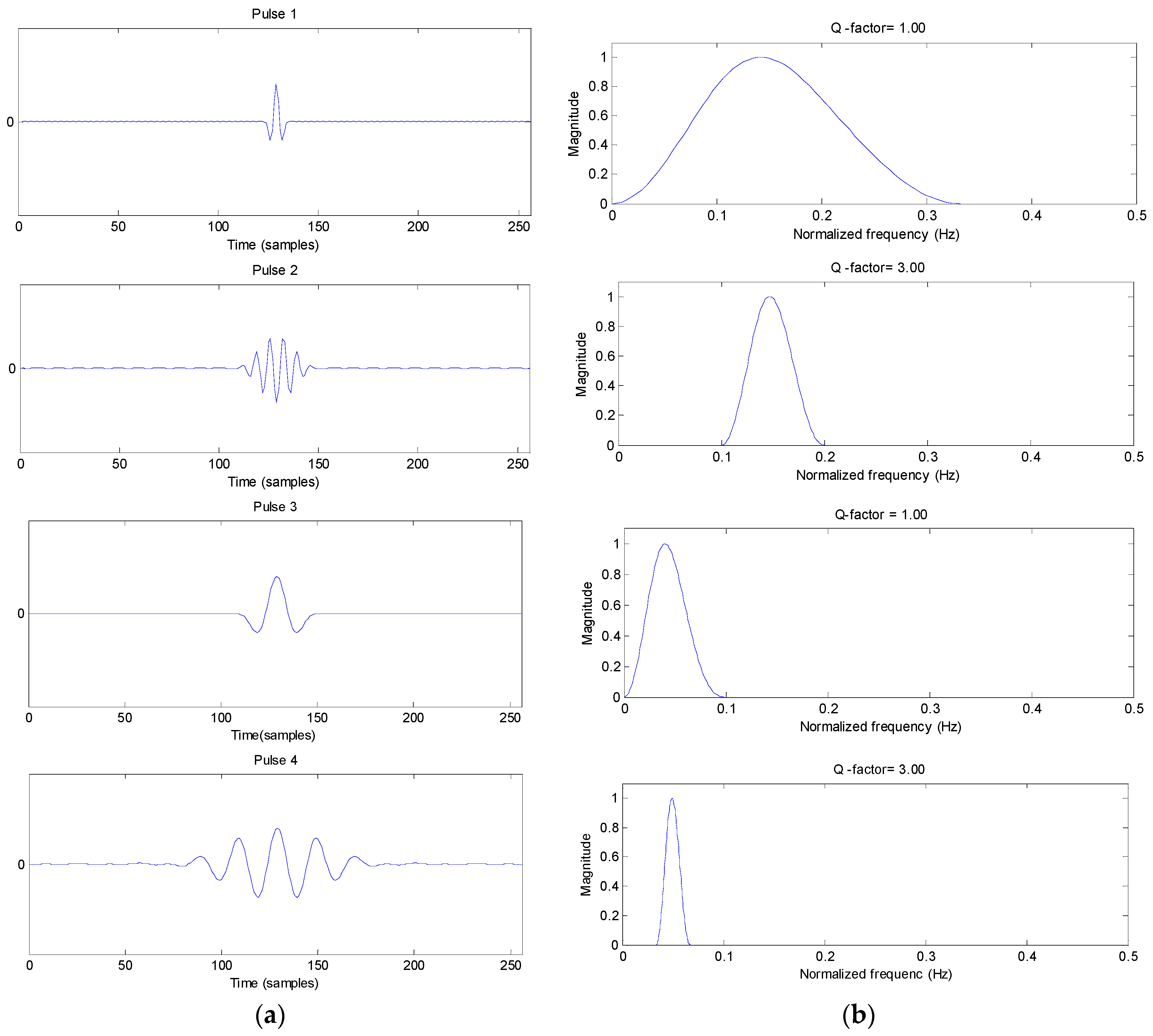
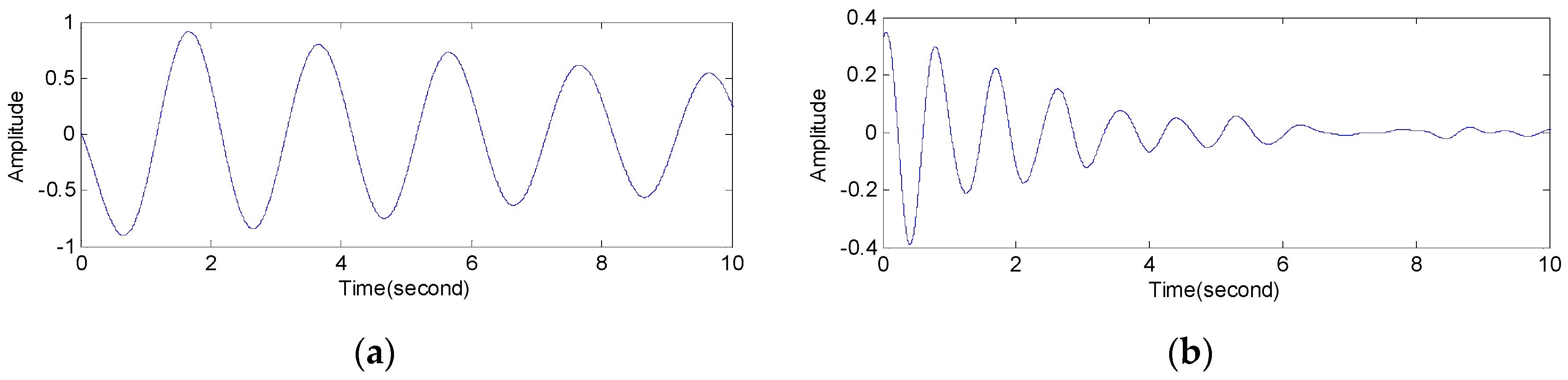
where f_c is the resonant frequency, B_w is the half-power bandwidth. Figure 1 illustrates the concept of signal resonance. Pulses 1 and 3, essentially a single cycle in duration, are low-resonance pulses because they do not exhibit sustained oscillatory behavior. Pulses 2 and 4, whose oscillations are more sustained, are high-resonance pulses. A low Q-factor wavelet transform is suitable for the efficient representation of pulses 1 and 3. The efficient representation of Pulses 2 and 4 calls for a wavelet transform with higher Q-factor.

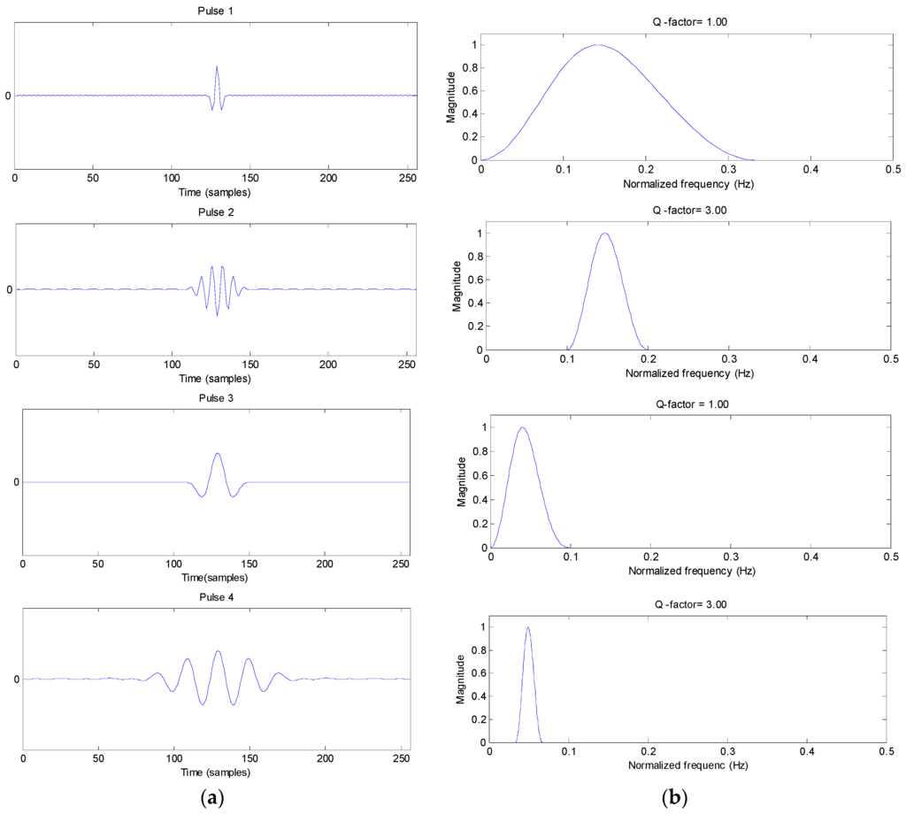
Figure 1. The resonance property of a signal. (a) Signals; (b) Frequency spectra.

2.1.2. LFO’s Resonance

Higher Q indicates a lower rate of energy loss relative to the stored energy of the resonator. The oscillations die out more slowly. Resonators with high quality factors have low damping. A system with high quality factor is said to be underdamped. Underdamped systems combine oscillations at a specific frequency with a decay of the signal amplitude.

A system with low quality factor is said to be overdamped. Such a system doesn't oscillate at all, but when displaced from its equilibrium steady-state output it returns to it by exponential decay, approaching the steady state value asymptotically.

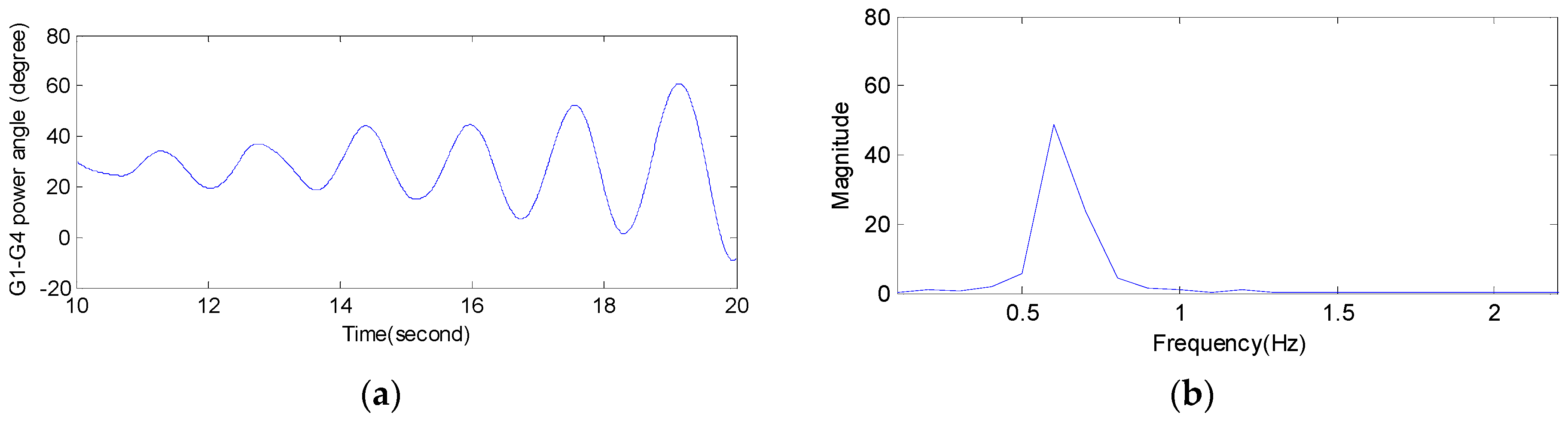
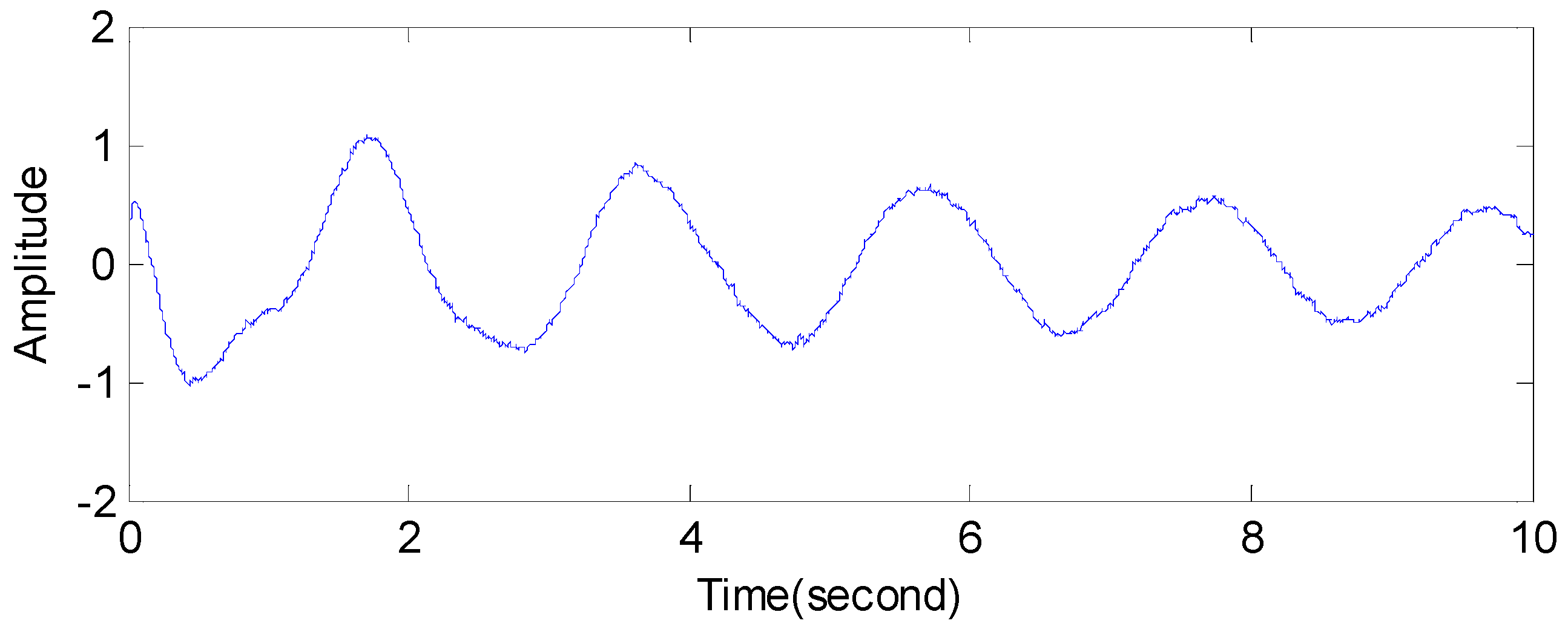
Figure 2 illustrates the resonance of the LFO signal, using Kunder’s four machine two area system as an example [11]. The signal is the relative power angle swing curve of generator 4 to generator 1. Thus, the LFO signal is the output of underdamped systems at a specific frequency with high Q-factor and high-resonance properties.

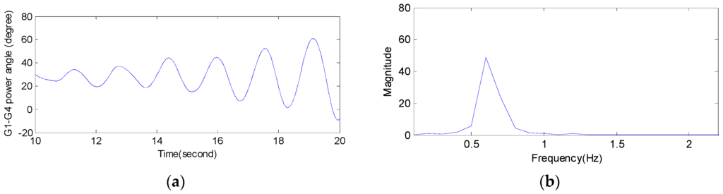
Figure 2. The resonance property of the LFO signal. (a) Power angle oscillation waveform of G4 relative to G1; (b) FFT frequency spectrum.

2.2. Tunable Q-Factor Wavelet Transform

TQWT is a flexible fully-discrete wavelet transform [12]. Hence, the transformation can be tuned according to the oscillatory behavior of the signal to which it is applied. The transformation is based on a real-valued scaling factor (dilation-factor) and implemented by a perfect reconstruction over-sampled filter bank with real-valued sampling factors [12].

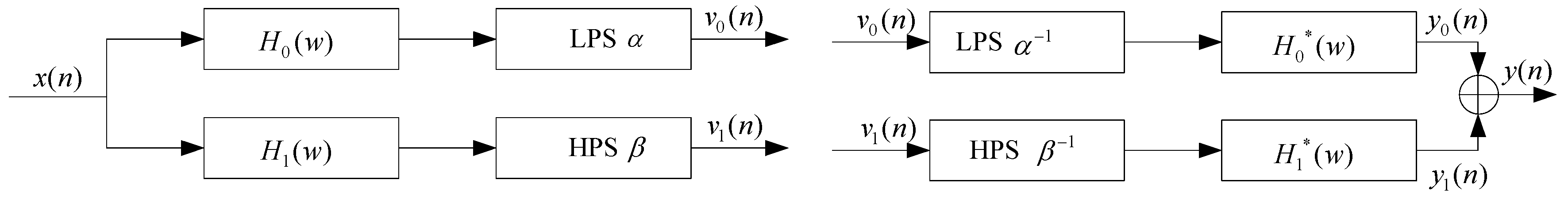
In Figure 3, the sub-band signal v₀(n) has a sampling rate of αf_s where f_s is the sampling rate of the input signal x(n). Likewise, the sub-band signal v₁(n) has a sampling rate of βf_s. LPS and HPS represent low-pass scaling and high-pass scaling, respectively.

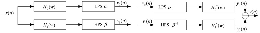
Figure 3. Analysis and synthesis filter banks for the TQWT.

The transfer functions of the blocks H₀(ω) and H₁(ω) are given by [12]:

$$H_0(\mathsf{\omega })=\{\begin{array}{l}1\hfill \\ \mathsf{\theta }(\frac{\mathsf{\omega }+(\mathsf{\beta }-1)\mathsf{\pi }}{\mathsf{\alpha }+\mathsf{\beta }-1})\hfill \\ 0\hfill \end{array}\begin{array}{c}\left|\mathsf{\omega }\right|\le (1-\mathsf{\beta })\mathsf{\pi }\\ (1-\mathsf{\beta })\mathsf{\pi }\le \left|\mathsf{\omega }\right|\le \mathsf{\alpha }\mathsf{\pi }\\ \mathsf{\alpha }\mathsf{\pi }\le \left|\mathsf{\omega }\right|\le \mathsf{\pi }\end{array}$$

(2)

$$H_1(\mathsf{\omega })=\{\begin{array}{l}0\hfill \\ \mathsf{\theta }(\frac{\mathsf{\alpha }\mathsf{\pi }-\mathsf{\omega }}{\mathsf{\alpha }+\mathsf{\beta }-1})\hfill \\ 1\hfill \end{array}\begin{array}{c}\left|\mathsf{\omega }\right|\le (1-\mathsf{\beta })\mathsf{\pi }\\ (1-\mathsf{\beta })\mathsf{\pi }\le \left|\mathsf{\omega }\right|\le \mathsf{\alpha }\mathsf{\pi }\\ \mathsf{\alpha }\mathsf{\pi }\le \left|\mathsf{\omega }\right|\le \mathsf{\pi }\end{array}$$

(3)

where $0<\mathsf{\alpha }<1$, $0<\mathsf{\beta }\le 1$, $\mathsf{\alpha }+\mathsf{\beta }>1$, $\mathsf{\theta }(\mathsf{\omega })=1/2(1+\cos \mathsf{\omega })\sqrt{2-\cos \mathsf{\omega }}$, $\left|\mathsf{\omega }\right|\le \mathsf{\pi }$. Scaling factors α and β can be expressed in terms of the Q-factor and redundancy r [12]: $\mathsf{\beta }=2/(Q+1)$, $\mathsf{\alpha }=1-\mathsf{\beta }/r$.

The main parameters for the TQWT are the Q-factor Q, the redundancy r, and the number of stages (or levels) J. Generally, Q is a measure of the number of oscillations the wavelet exhibits. A high Q-factor wavelet transformation requires more levels to cover the same frequency range compared with a low Q-factor transformation. We use Q = 1 for non-oscillatory signals. A higher value of Q is appropriate for oscillatory signals. The parameter r is the redundancy of the TQWT when it is computed by infinitely many levels. Generally, a value of r = 3 is recommended. Meanwhile, it can be interpreted as a measure of how much spectral overlap exists between adjacent band-pass filters. Increasing r has the effect on increasing overlapping in the frequency domain of the band-pass filters constituting the TQWT. The parameter J denotes the number of filter banks. There will be J + 1 sub-bands: the high-pass filter output signal of each filter bank, and the low-pass filter output signal of the final filter bank.

2.3. Morphological Component Analysis

Sparse signal processing exploits sparse representations of signals for applications such as denoising, deconvolution, signal separation, classification, etc. Therefore, the transformations for the sparse representation of signals is the key ingredient for sparse signal processing. In the noisy case, we should not ask for exact equality. Given an observed signal:

x = x₁ + x₂ + n, with x, x₁, x₂ ∈ R^N

(4)

where n is noise. The goal of Morphological Component Analysis (MCA) is to estimate/determine x₁ and x₂ individually. Assuming that x₁ and x₂ can could be sparsely represented in bases (or frames) Φ₁ and Φ₂ respectively, they can be estimated by minimizing the objective function:

$$J(w_1,w_2)={\mathsf{\lambda }}_1{\Vert w_1\Vert }_1+{\mathsf{\lambda }}_2{\Vert w_2\Vert }_1$$

(5)

respect to w₁ and w₂, subject to the constraint:

$${\mathsf{\Phi }}_1{w}_1+{\mathsf{\Phi }}_2{w}_2=x$$

(6)

Then MCA provides the estimates:

$${\widehat{x}}_1={\mathsf{\Phi }}_1{w}_1$$

(7)

and:

$${\widehat{x}}_2={\mathsf{\Phi }}_2{w}_2$$

(8)

We apply a variant of the split augmented Lagrangian shrinkage algorithm (SALSA) [13] to solve the MCA problem with iterative algorithm.

3. Frequency Slice Wavelet Transform

3.1. The Definition of Frequency Slice Wavelet Transform

Suppose $\widehat{p}(\mathsf{\omega })$ is the Fourier transformation of the function p(t). For $f(t)\in L^2(R)$, the FSWT is defined directly in the frequency domain as:

$$W(t,\mathsf{\omega },\mathsf{\lambda },\mathsf{\sigma })=\frac{1}{2\mathsf{\pi }}\mathsf{\lambda }{\displaystyle {\int }_{-\infty }^{+\infty }\widehat{f}(u)\widehat{p}(\frac{u-\mathsf{\omega }}{\mathsf{\sigma }}})e^{iut}du$$

(9)

where the scale σ ≠ 0 and energy coefficient λ ≠ 0 are constants or are functions of ω and t. The star “*” means the conjugate of a function. The general wavelet is a “microscope” in the time domain, but here FSWT is a “microscope” in the frequency domain, and this transformation is also named the wavelet transform in frequency domain [7,8].

$\widehat{p}(\mathsf{\omega })$ also called a frequency slice function (FSF) [7]. By using the Parseval equation, if σ is not the function of the assessed frequency u then Equation (9) can be translated into its time domain [8]:

$$W(t,\mathsf{\omega },\mathsf{\lambda },\mathsf{\sigma })=\mathsf{\sigma }\mathsf{\lambda }{e}^{i\mathsf{\omega }t}{\displaystyle {\int }_{-\infty }^{+\infty }f(\mathsf{\tau })e^{-i\mathsf{\omega }\mathsf{\tau }}{p}^{*}(\mathsf{\sigma }(\mathsf{\tau }-t)})d\mathsf{\tau }$$

(10)

We are not concerned with the definition of Equation (10) in the time domain because it is not easy to analyze in the frequency domain, even if we know the function type of $p(t)$ or its $\widehat{p}(\mathsf{\omega })$. Hence, we pay more attention to the function $\widehat{p}(\mathsf{\omega })$. Here, $\widehat{p}(\mathsf{\omega })$ is a frequency slice function (FSF), also called a frequency modulated signal or a filter. According to the Morlet transformation idea, taking σ = (ω/κ) (κ > 0), Equation (8) can be changed into:

$$W(t,\mathsf{\omega },\mathsf{\lambda },\mathsf{\kappa })=\frac{1}{2\mathsf{\pi }}\mathsf{\lambda }{\displaystyle {\int }_{-\infty }^{+\infty }\widehat{f}(u){\widehat{p}}^{*}(\mathsf{\kappa }\frac{u-\mathsf{\omega }}{\mathsf{\sigma }}})e^{iut}du$$

(11)

Note that the parameter κ in Equation (11) is a unique parameter that should be chosen in the application:

$$\mathsf{\kappa }=\frac{\Delta {\mathsf{\omega }}_p}{{\mathsf{\eta }}_s}$$

(12)

where η_s is frequency resolution ratio. Δω_p is the width of frequency window of FSF. As stated above in Equation (11), FSWT has another important property: FSWT can be controlled by the frequency resolution ratio η_s of the measured signal.

3.2. Frequency Slice Wavelet Inverse Transform

If $\widehat{p}(\mathsf{\omega })$ satisfies $\widehat{p}(0)=1$, then the original signal f(t) can be reconstructed by:

$$f(t)=\frac{1}{2\mathsf{\pi }\mathsf{\lambda }}{\displaystyle {\int }_{-\infty }^{+\infty }{\displaystyle {\int }_{-\infty }^{+\infty }W(\mathsf{\tau },\mathsf{\omega },\mathsf{\lambda },\mathsf{\sigma })e^{-i\mathsf{\omega }(t-\mathsf{\tau })}}}d\mathsf{\tau }d\mathsf{\sigma }$$

(13)

As an important result of Equation (10), the reconstruction procedure is independent from the selected FSF. Reconstruction independency is an important feature in FSWT, but this characteristic is not allowable in traditional wavelets.

Particularly, the signal component in the time-frequency area (t₁, t₂, ω₁, ω₂) is as below[14]:

$$f_x(t)=\frac{1}{2\mathsf{\pi }\mathsf{\lambda }}{\displaystyle {\int }_{{\mathsf{\omega }}_1}^{{\mathsf{\omega }}_2}{\displaystyle {\int }_{t_1}^{t_2}W(\mathsf{\tau },\mathsf{\omega },\mathsf{\lambda },\mathsf{\sigma })e^{-i\mathsf{\omega }(t-\mathsf{\tau })}}}d\mathsf{\tau }d\mathsf{\sigma }$$

(14)

FSWT provides a new approach whereby both filtering and segmenting can be processed simultaneously in the time and frequency domain.

4. Procedure of the LFO Time-Frequency Analysis Method Using RSSD and FSWT

Figure 4 is the flow chart of the proposed method.

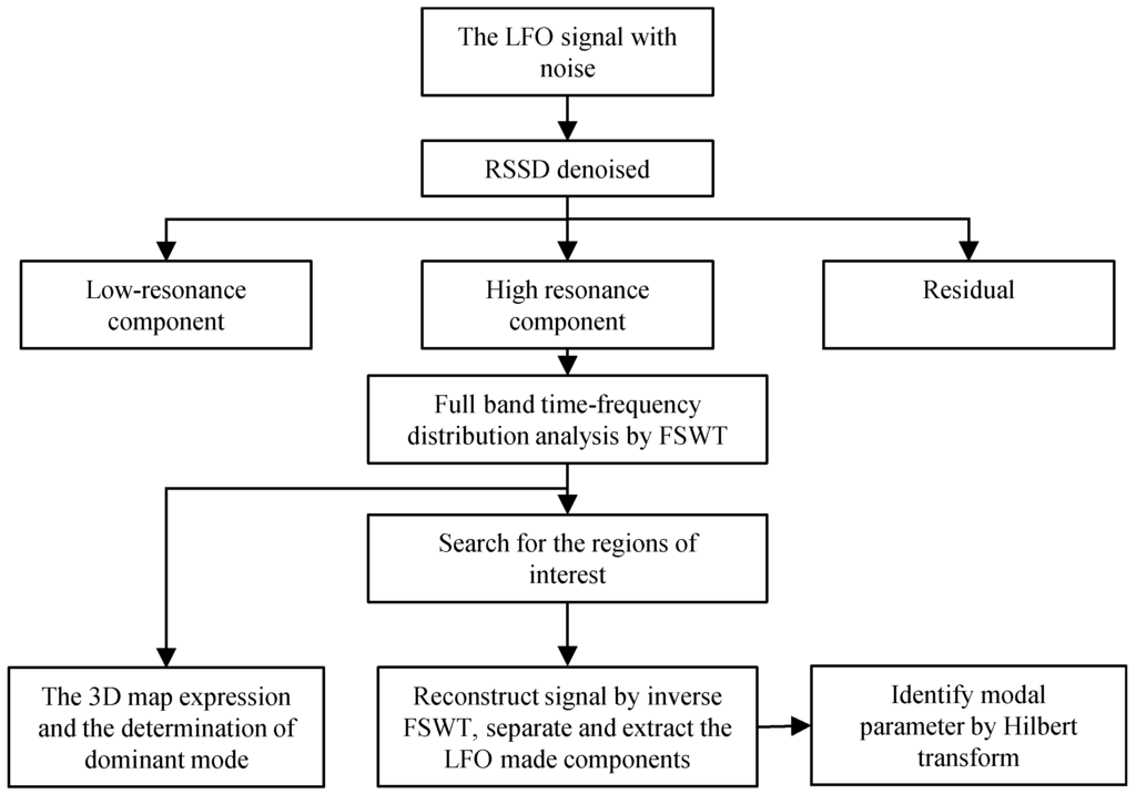
Figure 4. The flow chart of the LFO time-frequency analysis method using RSSD and FSWT.

In summary, the method procedure is divided into the following steps:

(1)

Decompose the LFO signal with noise by RSSD and get a high-resonance component, a low-resonance component and a residual. The high-resonance component is de-noised LFO signal.

(2)

Transform the high-resonance component by FSWT, and compute the FSWT coefficients using Equation (9), and obtain the full band of its time-frequency distribution. The 3D map expression and dominant mode of the LFO signal can be obtained. After that, search for the regions of interest, called modal domains, in which the main energy is concentrated. Chose a frequency slice [ω_i, ω_i+1] to get an accurate analysis of the time-frequency feature. Separate and extract the LFO mode components through reconstructing signals by inverse FSWT.

(3)

Identify the parameters of the LFO mode components by Hilbert transform (HT). With the HT method, the LFO mode component’s oscillation frequency and damping ratio are obtained. Readers may refer to [15,16] for the details of the HT method.

5. Simulation

5.1. Denoised RSSD

5.1.1. Example 1

The LFO signal can be approximated by:

$$x(t)={\displaystyle \sum _{i=1}^n{A}_i{e}^{{\mathsf{\sigma }}_{i}t}}\cos (2\mathsf{\pi }{f}_{i}t+{\mathsf{\varphi }}_i)+\mathsf{\lambda }(t)$$

(15)

where A_i is the amplitude, f_i is the oscillation frequency, σ_i is damping factor, Φi is the phase shift, λ(t) is white noise and σ its standard deviation. We set a f_s = 1000 Hz, T_s = 10 s and σ = 0.1. A signal simulated with Equation (15) is described in Table 1. There are two oscillation modes of the simulated signal. One is an inter-area oscillation mode in low frequency and the other is an intra-area oscillation mode in high frequency.

Table 1. The parameters of the simulated signal in Equation (15).

LFO Mode	Amplitude (Ai)	Oscillation Frequency (fi)	Damping Ratio (ξi)	Damping Factor (σi)	Phase Shift (Φi)
1	1	0.5	0.02	0.0628	60°
2	0.5	1.1	0.07	0.4837	45°

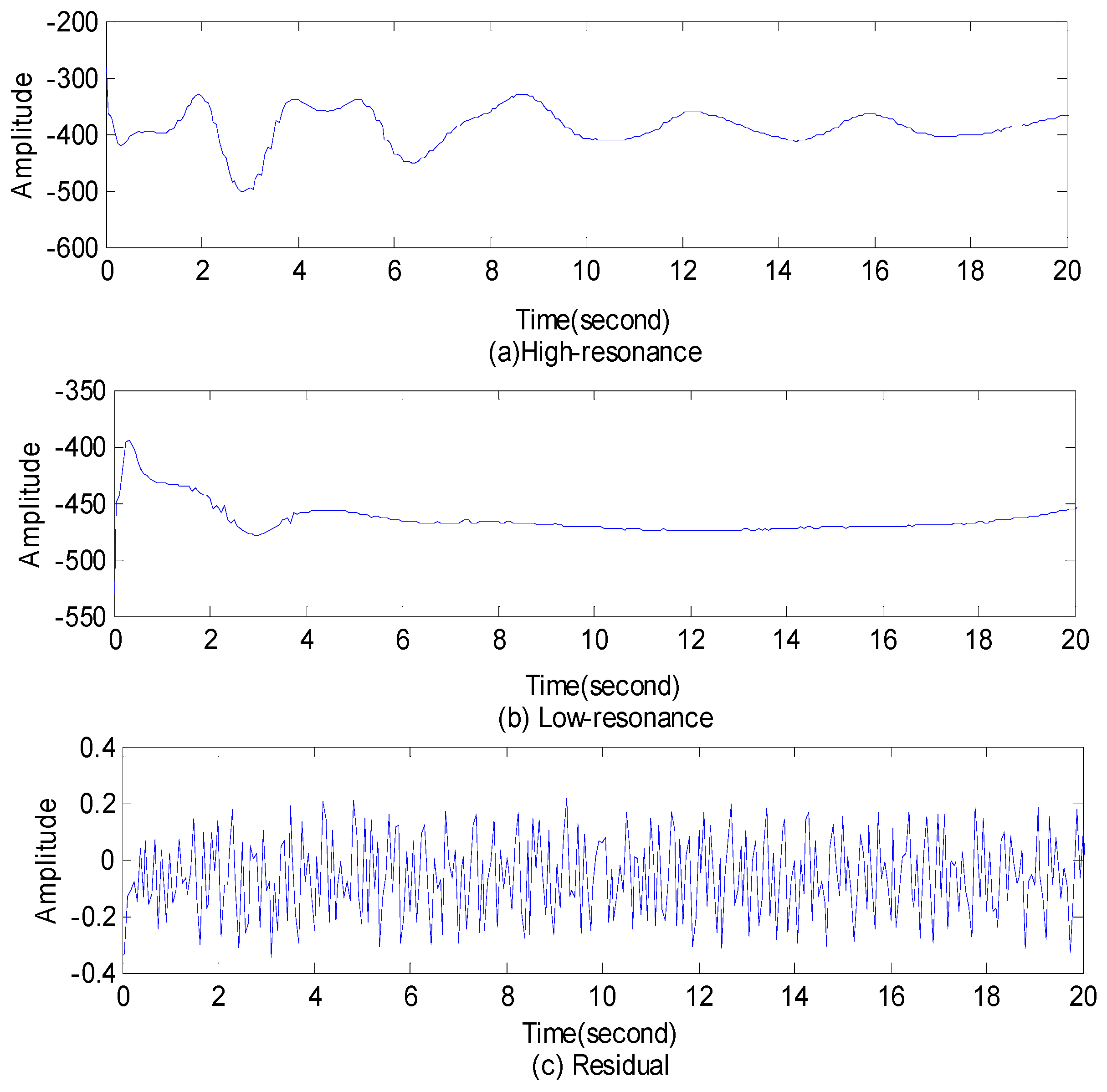
When the RSSD is applied to the simulated signal with Gaussian white noise, we get decomposition of the signal into high and a low-resonance components as seen in Figure 5. We use the parameters Q₁ =1, Q₂ = 4 and γ₁ = γ₂ = 3.

Figure 5. RSSD of the simulated signal with white Gaussian noise.

It can be seen from Figure 5 that this procedure separates the given signal into three signals that have quite different behavior. One signal (high-resonance component) is sparsely represented by a high Q-factor wavelet transform (Q = 4). The second signal (low-resonance component) is sparsely represented by a low Q-factor wavelet transform (Q = 1). The third signal (residual) is the signal component which is not sparsely represented in either the high Q-factor wavelet transformation or the low Q-factor wavelet transformation.

Note that the high-resonance component consists largely of sustained oscillatory behavior, and that is the denoised LFO signal, while the low-resonance component (in Figure 5, part (b)) looks like nearly zero, and almost no low-resonance component is there. The residual appears noise-like. The residual is mostly white Gaussian noise.

For quantifying the performance of RSSD de-noising, we calculated the root mean squared errors (RMSE) of the high-resonance signal and the ideal signal without noise .RMSE equals 0.6198. This proves that RSSD can remove white Gaussian noise well.

5.1.2. Example 2

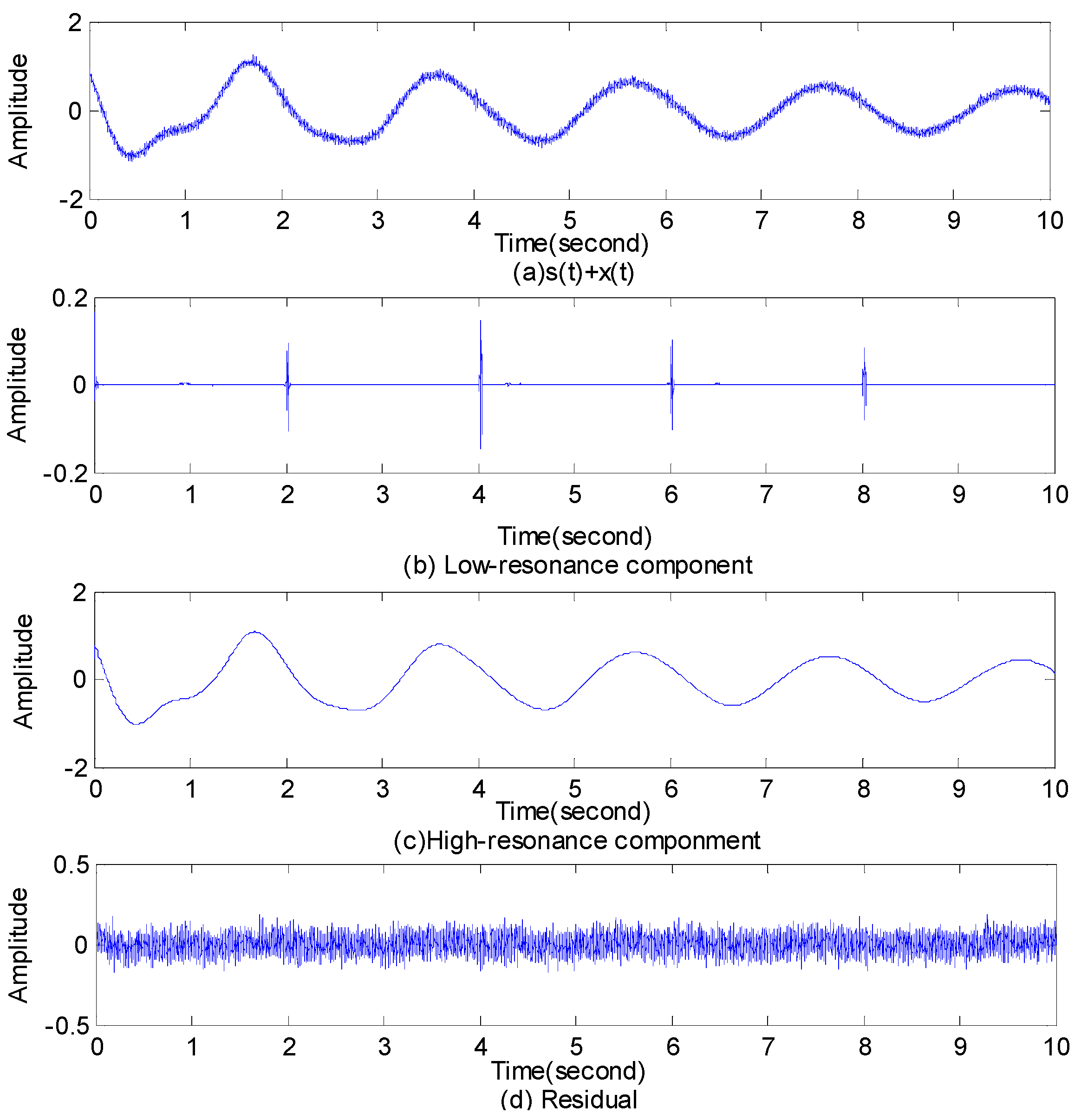
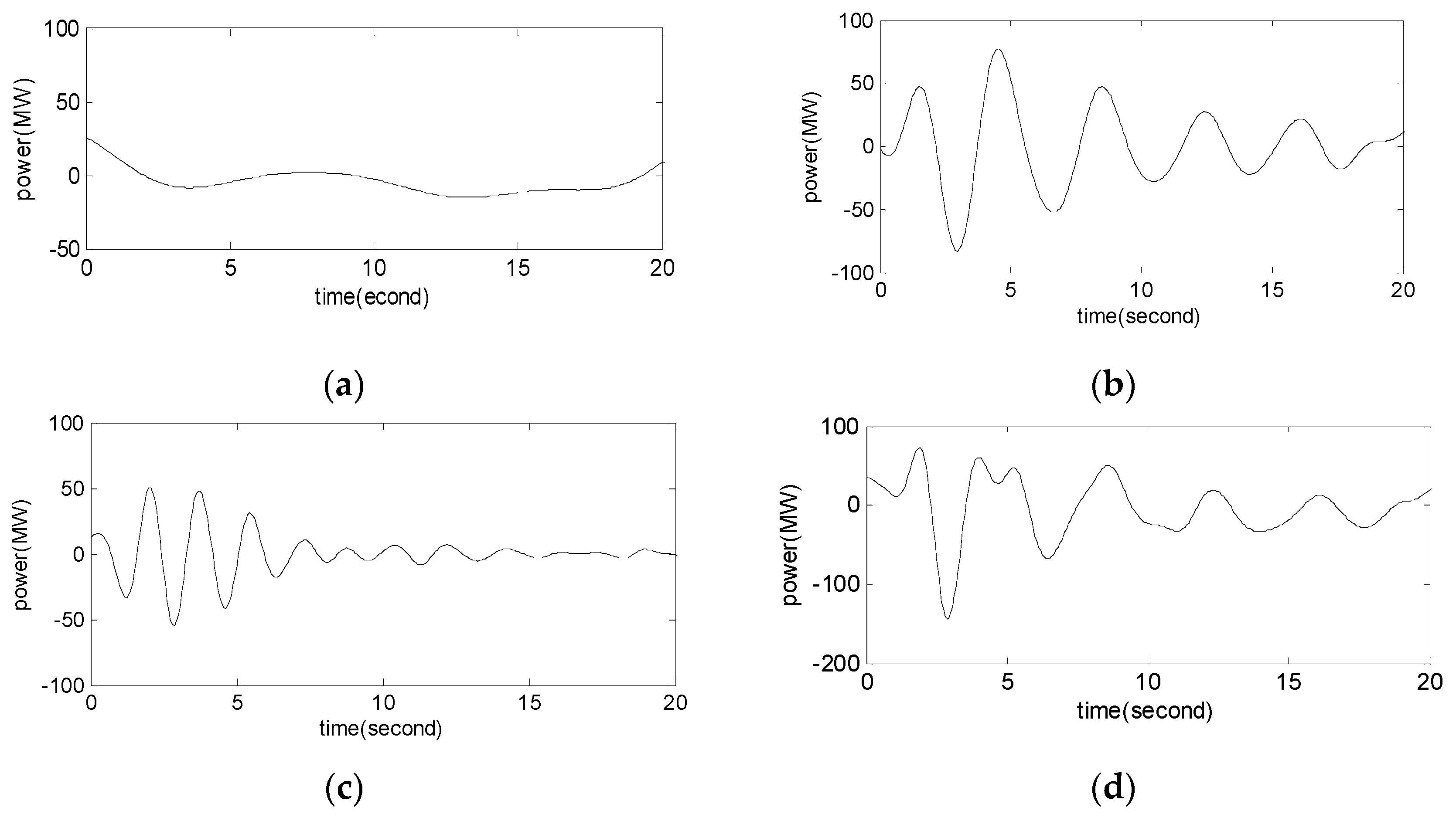
Add s(t) to the simulated signal of Example 1, and the LFO signal with transient impulse and noise is obtained as shown in Figure 6a. It’s worth noting that the components overlap in frequency:

$$s(t)=\{\begin{array}{l}0.1\sin 2\mathsf{\pi }\times 0.2t\text{\hspace{0.17em}\hspace{1em}\hspace{0.05em}\hspace{0.05em}\hspace{0.05em}}2 \mathrm{s}\le t\le 2.04 \mathrm{s},6 \mathrm{s}\le t\le 6.04 \mathrm{s}\hfill \\ 0.19\sin 2\mathsf{\pi }\times 0.5t4 \mathrm{s}\le t\le 4.08 \mathrm{s}\hfill \\ 0.08\sin 2\mathsf{\pi }\times 0.4t8 \mathrm{s}\le t\le 8.06 \mathrm{s}\hfill \\ 0\text{\hspace{1em}\hspace{1em}\hspace{1em}\hspace{1em}\hspace{1em}\hspace{1em}\hspace{1em}\hspace{1em}other}\hfill \end{array}$$

(16)

Figure 6. RSSD of the simulated signal with transient impulse and white noise.

It can be seen from Figure 6, part (b), that the low-resonance component is separated by RSSD. The low-resonance component consists largely of transients and oscillations that are not sustained, and that is exactly the transient impulse signal. The residual is mostly white Gaussian noise. Therefore, RSSD can successfully separate complex signals whose frequency bands are overlapped but differ in resonance properties.

5.2. FSWT Analysis

5.2.1. Full Band Time-Frequency Distribution Analysis by FSWT

Let the FSF be the Gaussian function $\widehat{p}(\mathsf{\omega })=e^{-\frac{1}{2}{\mathsf{\omega }}^2}$, hence $\Delta {\mathsf{\omega }}_p=\frac{\sqrt{2}}{2}$. Let $\mathsf{\kappa }=\frac{0.707}{\mathsf{\eta }}$ and set $\mathsf{\eta }=0.025$, hence $\mathsf{\kappa }=28.28$. The chosen parameters in FSWT are summarized as follows:

$$\widehat{p}(\mathsf{\omega })=e^{-\frac{1}{2}{\mathsf{\omega }}^2}, \mathsf{\sigma }=\frac{\mathsf{\omega }}{\mathsf{\kappa }}, \mathsf{\eta }=0.025, \mathsf{\kappa }=28.28$$

(17)

Considering the LFO’s frequency range, the frequency interval is from 0 Hz to 5 Hz. The full band time-frequency distribution analysis by FSWT is shown in Figure 7. The Fourier spectrum of the high-resonance component in Figure 7a shows that the first modal signal is a clear indication of the greatest energy at 0.5 Hz and other peaks at 1.1 Hz are smaller. Figure 7b,c shows the results of the 2D or 3D map of FSWT coefficients, where all of FSWT parameters are assumed in Equation (17). The damping characteristics of the signal in time-frequency domain are more clearly revealed in Figure 7c. Figure 7 reveals that FSWT has two clearly separated peaks that indicate two main modes. The first mode has the highest amplitude at about 0.5 Hz, while the second mode and not the first has the highest amplitude at about 1.1 Hz, so the LFO dominant mode is an oscillation mode of frequency 0.5 Hz.

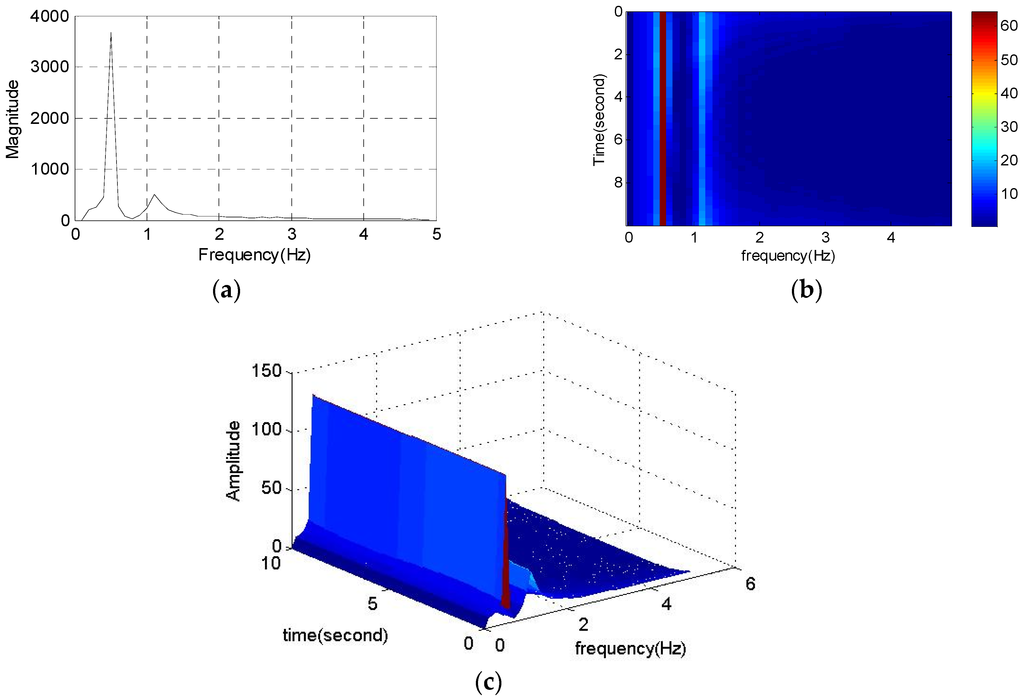
Figure 7. Full band time-frequency distribution analysis by FSWT. (a) Fourier spectrum; (b) The 2D maps of FSWT coefficients; (c) The 3D maps of FSWT coefficients.

5.2.2. Fine Analysis of Frequency Slices Based on FSWT

Accurate analysis of the time-frequency features is shown in Figure 8 and Figure 9. According to the analysis results of Figure 7, the chosen frequency slices are [0, 0.8] Hz and [0.8, 2] Hz, respectively. Note that each modal signal on the 2D map of FSWT coefficients is a connected area. This is an important feature for modal signal separation. Here the segments are not strict, but it is necessary that each slice include the main energy of one modal signal. We can reconstruct the objective signal through Equation (14). The reconstructed signals shown in Figure 8c and Figure 9c are good. There are only some differences in FSWT amplitudes. The end is not accurate reconstruction, because the reconstructed signal and the ideal signal do not perfectly match in the end, but this does not affect damping estimation, because the damping is only a ratio of the FSWT amplitudes.

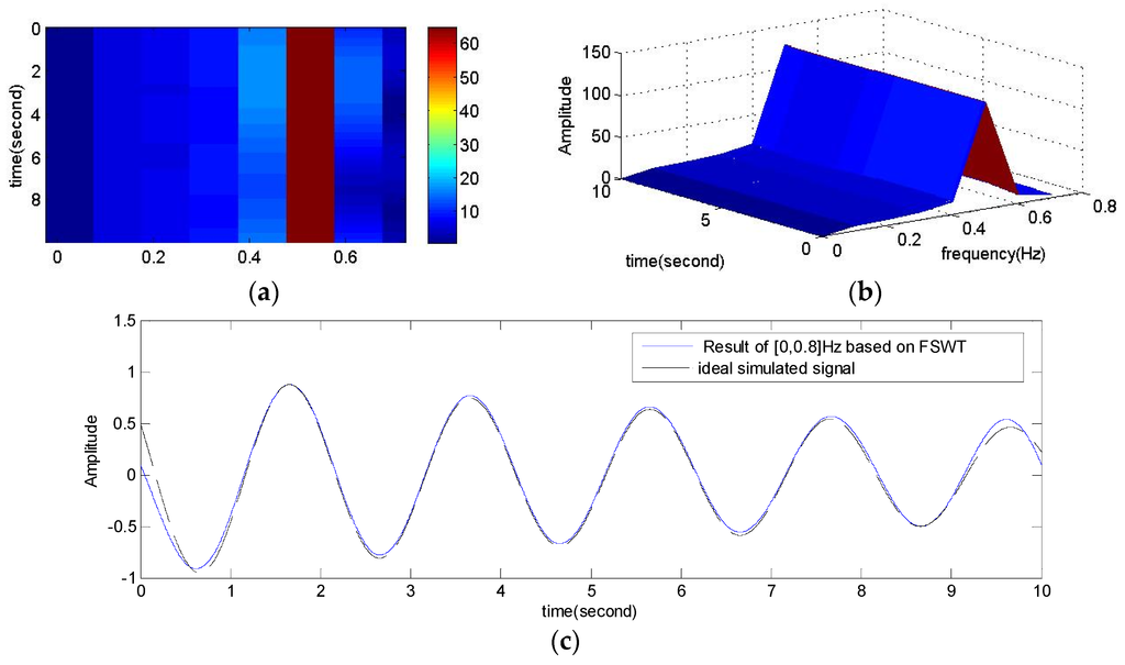
Figure 8. Fine analysis of frequency slice [0, 0.8] Hz based on FSWT. (a) FSWT 2D map; (b) FSWT 3D map; (c) Comparison of the reconstructed signal with the ideal signal.

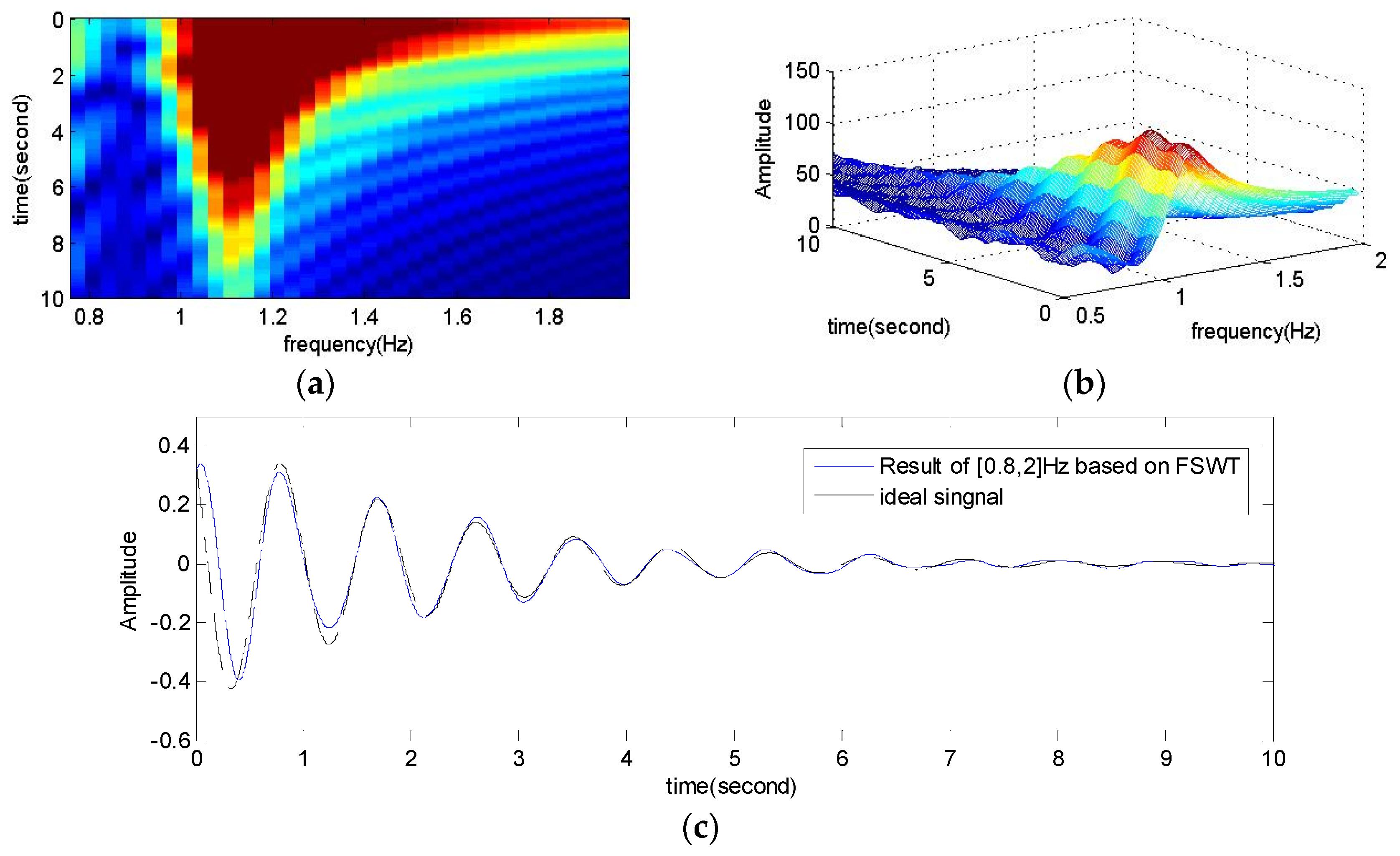
Figure 9. Fine analysis of frequency slice [0.8, 2] based on FSWT. (a) FSWT 2D map; (b) FSWT 3D map; (c) Comparison of the reconstructed signal with the ideal signal.

5.3. Identification of the Parameters of LFO Mode Components by HT

The reconstructed signals based on feature of frequency slice are the separated and extracted LFO mode components. We identify the parameters of mode components by the Hilbert transform. The results is shown in Table 2. The results shows that the identified results are relatively accurate and the error of the method is less than 5%.

Table 2. LFO mode components parameters after RSSD denoising (σ = 0.1).

Mode		True Value	FSWT-HT
			Identification Result	Error (%)
1	Oscillation frequency (Hz)	0.5000	0.4980	0.40
	Damping ratio	0.0200	0.0196	2.00
2	Oscillation frequency (Hz)	1.1000	1.1101	0.92
	Damping ratio	0.0700	0.0666	4.86

5.4. Impact of Noise on the Accuracy of FSWT-HT

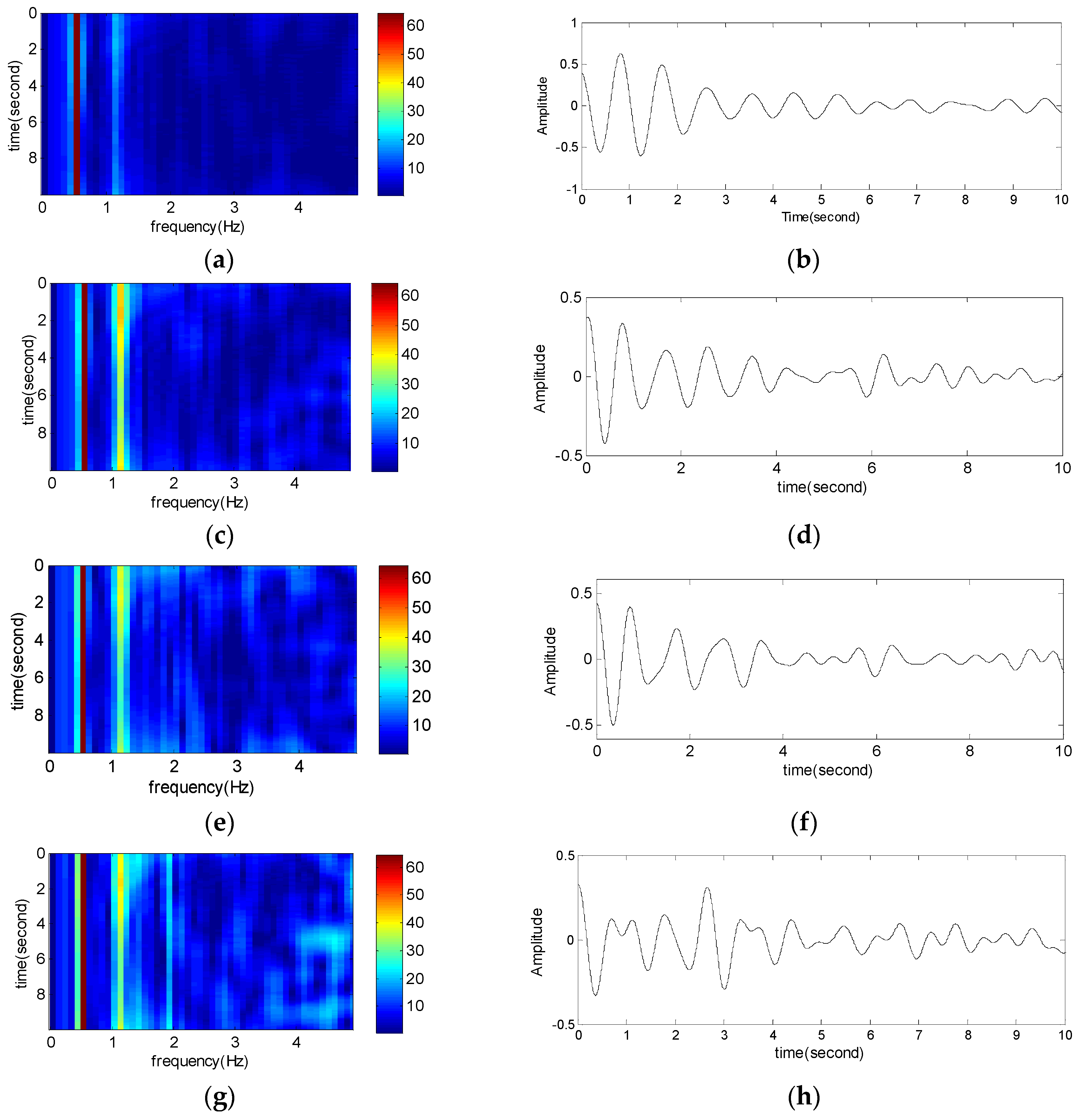
We change the noise level of Equation (15), and let the standard deviation (σ) equal 0.5, 1, 1.5 or 2, respectively. The full band time-frequency distribution analysis and fine analysis of the frequency-slice interval are shown in Figure 10.

Figure 10. Full band time-frequency distribution and Fine analysis of frequency slice based on FSWT. (a) FSWT 2D map (σ = 0.5); (b) Reconstructed signal of [0, 0.8] Hz; (c) FSWT 2D map (σ = 1); (d) Reconstructed signal of [0, 0.8] Hz; (e) FSWT 2D map (σ = 1.5); (f) Reconstructed signal of [0, 0.8] Hz; (g) FSWT 2D map (σ = 2); (h) Reconstructed signal of [0, 0.8] Hz.

As shown in Figure 10, noises do not affect the results of full band time-frequency analysis seriously. The time-frequency characteristics are not clear when the noise standard deviation σ = 2. This proves the FSWT method presents good performance against noise to a certain degree, but noise affects the amplitude of reconstructed signals, especially for the reconstructed signals of frequency from 0 to 0.8 Hz. Frequency slice equals a bandpass filter which removes other frequency interference, but the white noise of the frequency slice has not been completely removed, which may impact the accuracy of oscillation mode identification, especially for damping ratio. Results are shown in Table 3. Compared with Table 2, it is necessary to denoise the LFO signal by RSSD.

Table 3. Result of identification with white noise.

Mode	Standard Deviation (σ)	Oscillation Frequency (Hz)	Error (%)	Damping Ratio	Error (%)
1	0.1	0.4980	0.400	0.0188	6.000
2		1.1101	0.92	0.0657	6.143
1	0.5	0.4978	0.440	0.0190	5.000
2		1.1031	0.282	0.0637	9.000
1	1	0.4968	0.640	0.0181	9.500
2		1.1131	1.20	0.0613	12.429
1	1.5	0.4975	0.500	0.0171	14.500
2		1.1156	1.418	0.0571	18.428
1	2	0.4977	0.460	0.0170	15.000
2		1.1221	2.009	0.0470	32.857

5.5. Comparison with Low Pass Filtering

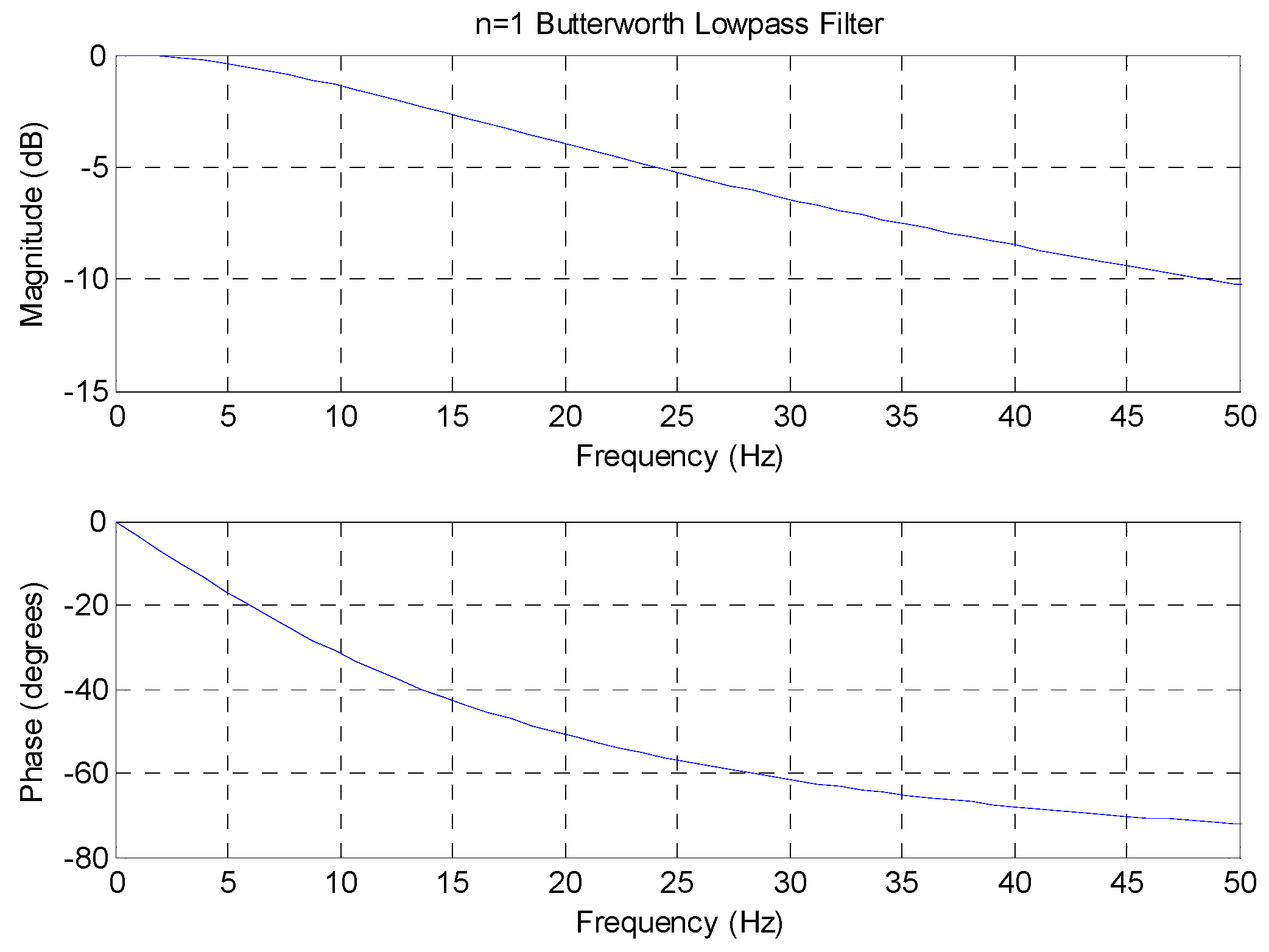
We design a Butterworth low-pass filter with less than 3 dB of ripple in the passband, defined frequency from 0 to 2.5 Hz, and at least 20 dB of attenuation in the stopband, defined from 150 Hz to the Nyquist frequency (500 Hz). Transfer function is:

$$H(z)=\frac{0.0487(1+Z^{-1})}{1-0.9026Z^{-1}}$$

(18)

The frequency response of the filter is plotted that illustrates in Figure 11.

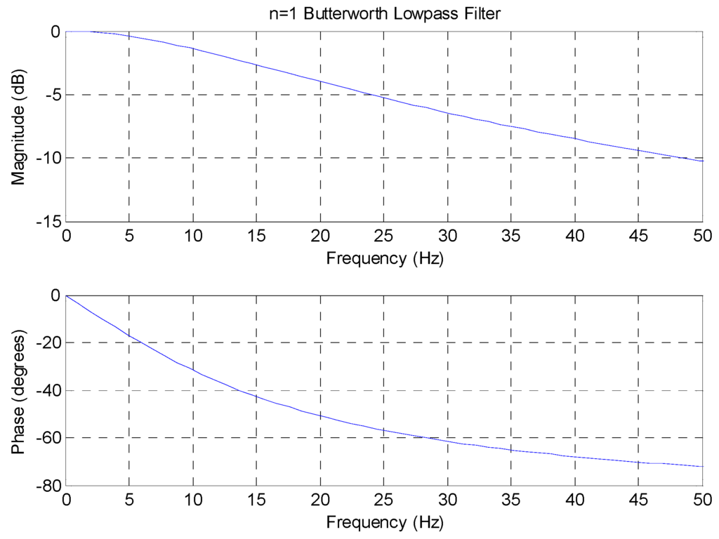
Figure 11. Frequency characteristics of a Butterworth low-pass filter.

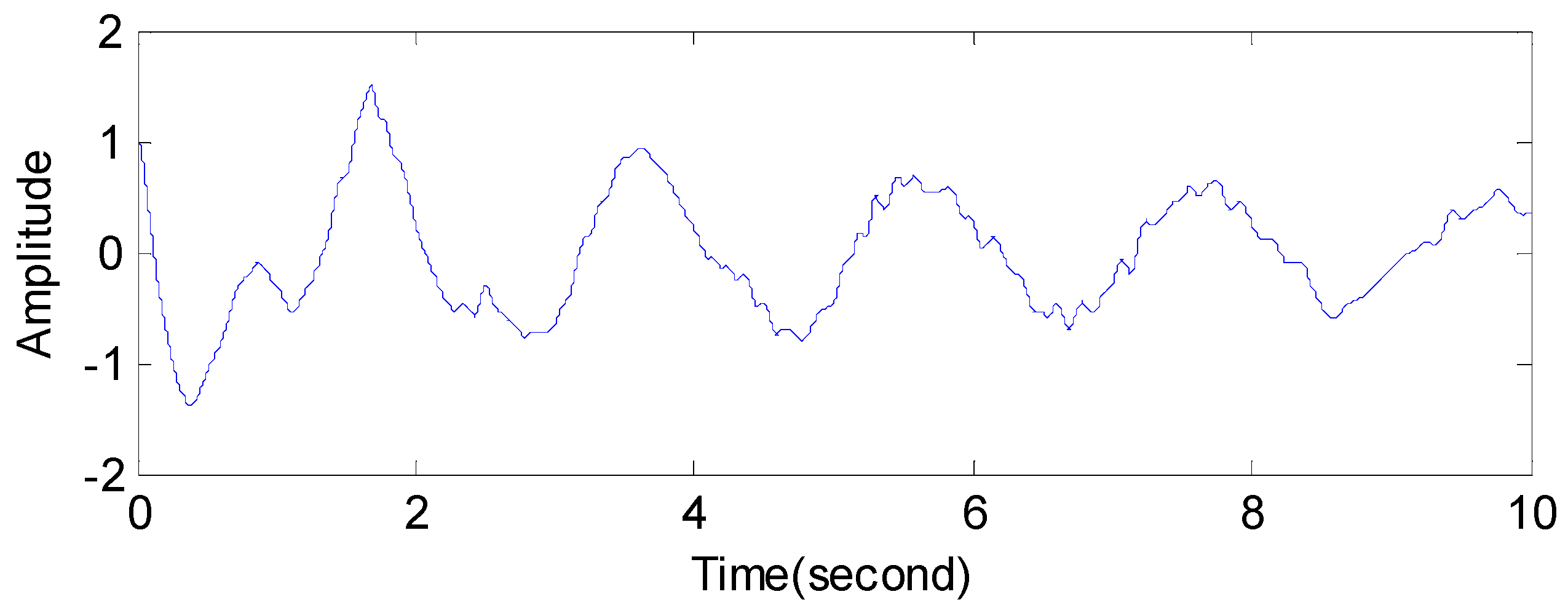
After the simulated signal with white Gaussian noise of Equation (15) is processed through a low-pass filter, we obtain a signal with colored Gaussian noise, which can be seen in Figure 12. Choose frequency slices are [0, 0.8] Hz and [0.8, 2] Hz, respectively. The reconstructed signals are shown in Figure 13.

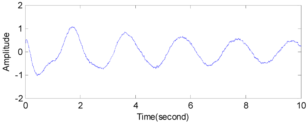
Figure 12. The simulated signal with colored noise after low-pass filtering.

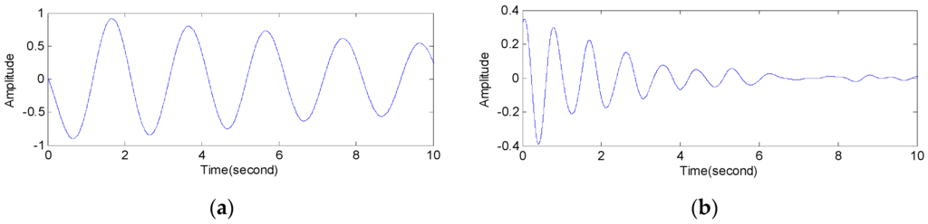
Figure 13. Fine analysis of the simulated signal with colored noise based on FSWT. (a) Frequency slice [0, 0.8] Hz; (b) Frequency slice [0, 0.8] Hz.

Comparing Figure 5c and Figure 12, it is clear that the RSSD method denoises the LFO signal better. It can be seen that although the white Gaussian noise changes to colored one, low frequency noise interference still exists. The reconstructed results are similar to Example 1 with white Gaussian noise.

It is thus indicated that low-pass filtering is not effective as a denoising pretreatment of FSWT. On the one hand, it is also shows that both colored and white noise may impact the accuracy of the oscillation mode identification of FSWT-HT and denoising the LFO signal by RSSD is necessary.

5.6. Comparison with Other Parameter Identification Methods

In order to validate the effectiveness of the proposed method, it is compared with the Prony [17], stochastic subspace identification (SSI) [18], empirical mode decomposition (EMD) and SSI (EMD-SSI) [19], and RSSD-SSI methods. The simulated signal is the one of Equation (15), which the standard deviation (σ) equals 0.5. The number of simulation trials is 100. The results are shown in Table 4.

Table 4. Result of identification with Gaussian noise (σ = 0.5).

Method	Mode	Oscillation Frequency (Hz)	Error (%)	Damping Ratio	Error (%)
Prony	1	0.4502	9.960	0.0240	20.00
	2	1.1616	5.609	0.0580	17.14
SSI	1	0.4766	4.680	0.0222	11.00
	2	1.1573	5.209	0.0753	7.571
EMD-SSI	1	0.4860	2.800	0.0214	7.000
	2	1.1502	4.727	0.0743	6.142
RSSD-SSI	1	0.5060	1.200	0.0206	3.000
	2	1.1302	2.745	0.0730	2.857
RSSD-FSWT	1	0.4978	0.440	0.0192	4.000
	2	1.1030	0.272	0.0667	4.714

As can be seen from Table 4 below, the identified results of the RSSD-FSWT and RSSD-SSI methods are ranked most accurate, followed by EMD-SSI, SSI and Prony. The Prony method is the worst. Since traditional Prony method is sensitive to the noise of data [20,21]. The existence of noise in the signal will leads to a larger error in the results of Prony algorithm.

SSI is a novel approach that developed in recent years. It can identify modal parameters of linear structures from ambient structure vibrations [22]. The SSI method is recently applied to the identification of LFO modes. For singular value decomposition (SVD) is the main step of SSI, the method is more satisfactory than traditional methods, as its higher accuracy and better noise immunity. There are two stable oscillation modes, and considering the noise, the order of SSI can be set to 6, the frequency tole is 1%. But if the noise is strong (the signal-to-noise ratio,SNR is lower than 10 dB), denoising pretreatment is necessary [23].The SNR of this example is 0.2210 dB. So in this case, the result of SSI is better than Prony, but it is not as good as the EMD-SSI and RSSD-SSI methods.

The EMD-SSI method means that the signal denoised by EMD first,and then the SSI method is employed to identify modal parameters of the LFO signal. The similar RSSD-SSI method means SSI after RSSD. Compared the results between the EMD-SSI and RSSD-SSI methods, the latter is better than the former. The EMD method is a relatively new tool for the nonlinear and non-stationary signals analysis, and it can adaptively decompose signals into several intrinsic mode functions (IMFs) according to its characteristic time scale. It starts from the data itself to decompose the signals in spatial domain, so it can discriminate the signals from the noise. But the EMD method contains some theoretical problems, such as envelop and mean curve fit, boundary effect, modes mix and so on, which affect its application. The result of EMD threshold de-noising[24] is showed in Figure 14. The LFO signal is decomposed into 16 IMFs and a residue.

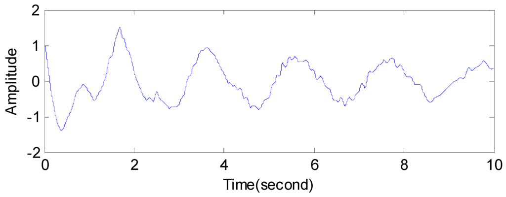
Figure 14. The simulated signal after EMD threshold de-noising.

From Table 4, both of the RSSD-SSI and RSSD-FSWT methods have high accuracy in the identification of the oscillation frequency and damping ratio. RSSD-SSI is the best at estimating damping ratio while RSSD-FWST gives a better estimate of oscillation frequency.

6. Engineering Application

In this section, the proposed method is applied to an engineering application. In order to validate the effectiveness of the proposed method, it is compared with the RSSD-SSI and EMD-SSI methods [19]. The measured power oscillation waveform in Figure 15 is the active power data of the Jiangjiaying-Gaojiang 1st line from a 3.29 large-disturbance testing scheme for the Northeast China power grid. The data have been filtered by low-pass filtering.

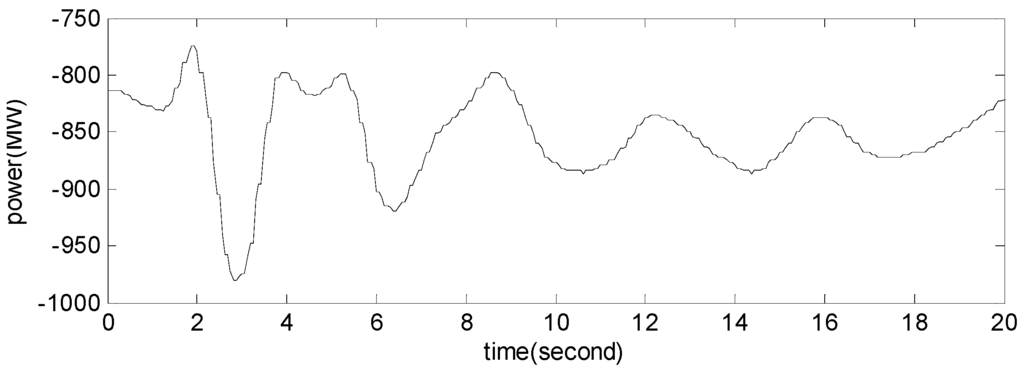
Figure 15. Active power of the Jiangjiaying-Gaojiang 1st line.

Firstly, RSSD is applied to active power data; the high-resonance component in Figure 16b is the denoised data. We used the parameters Q₁ =1, Q₂ = 4, ${\mathsf{\gamma }}_1={\mathsf{\gamma }}_2=3$.

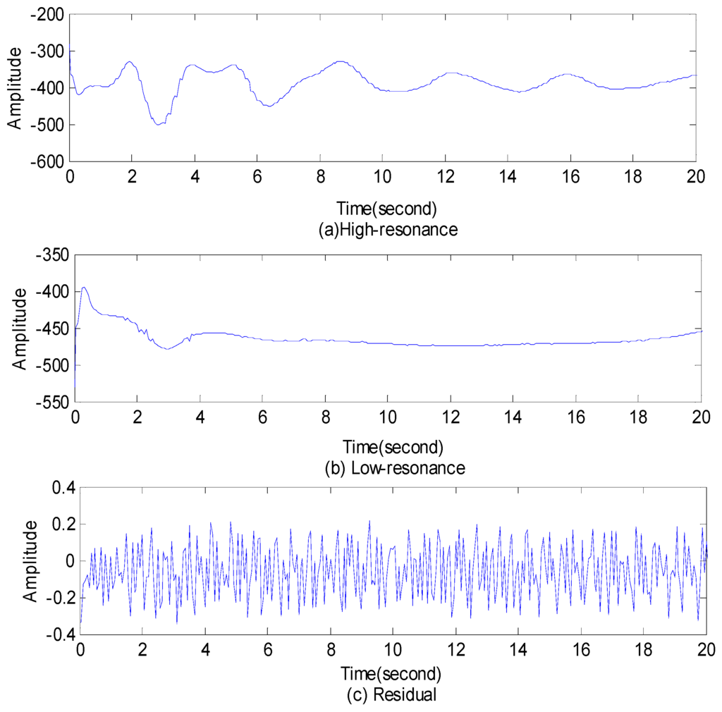
Figure 16. RSSD of power oscillation waveform of the Jiangjiaying-Gaojiang line 1st.

Full band time-frequency distribution analysis by FSWT is shown in Figure 17. Three frequency component amplitudes are prominent. They are 0.54 Hz, 0.25 Hz, and 0.12 Hz, respectively. There are three main modes. The highest amplitude is at about 0.25 Hz, so the LFO dominant mode is the 0.25 Hz oscillation mode.

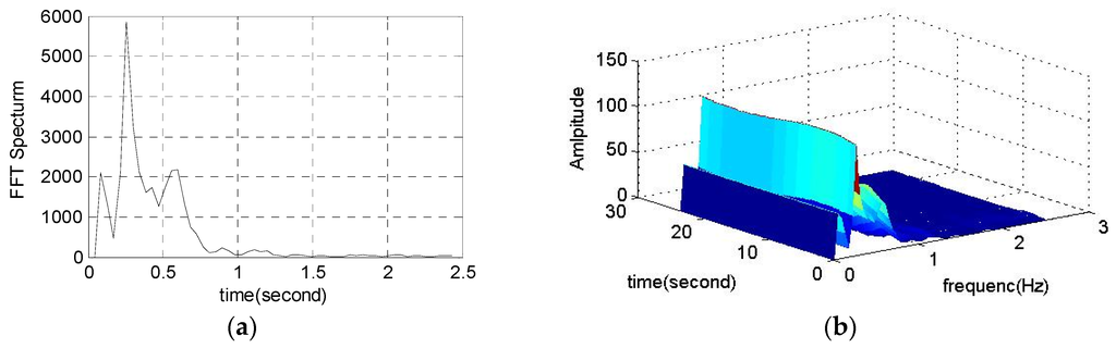
Figure 17. Full band time-frequency distribution analysis by FSWT. (a) FFT spectrum; (b) FSWT 3D map.

Frequency slice intervals are chosen [0, 0.2] Hz, [0.2, 0.5] Hz, and [0.8, 2] Hz, respectively. The multi-modals LFO signal can be separated into three single modes. The reconstructed signals are shown in Figure 18.

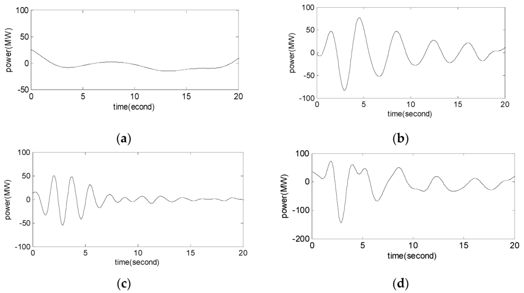
Figure 18. Fine analysis of frequency slices based on FSWT. (a) Reconstructed signal of [0, 0.2] Hz; (b) Reconstructed signal of [0.2, 0.5] Hz; (c) Reconstructed signal of [0.8, 2] Hz; (d) Reconstructed signal = (a) + (b) + (c).

We identify the parameters of three mode components by the Hilbert transform. The results are shown in Table 5. The results of parameters identified by the RSSD-SSI and EMD-SSI methods are also shown in Table 5. The fourth modal component is identified by EMD-SSI, but not detected by RSSD-FSWT and RSSD-SSI. The fourth modal component may be the false component which produced during the process of cubic spline curve fitting using EMD. Even if the fourth modal component is existent, the oscillation frequency (0.0411 Hz) is rather low, and the damping ratio is relatively high. Thus, the energy of the fourth modal component is very small and has negligible impact on the system. In other words, it does not play an important role in engineering application. Furthermore the RSSD-FSWT method has as high accuracy in the identification of the oscillation frequency and damping ratio as the other two methods.

Table 5. Parameters of low frequency oscillation mode.

Mode		Oscillation Frequency (Hz)	Damping Ratio
1	RSSD-SSI	0.5356	0.0556
	RSSD-FSWT	0.5244	0.0542
	EMD-SSI	05354	0.0571
2	RSSD-SSI	0.2510	0.0541
	RSSD-FSWT	0.2508	0.0538
	EMD-SSI	0.2658	0.0562
3	RSSD-SSI	0.1220	0.0149
	RSSD-FSWT	0.1215	0.0145
	EMD-SSI	0.1199	0.0123
4	RSSD-SSI	-	-
	RSSD-FSWT	-	-
	EMD-SSI	0.0411	0.0993

7. Concluding Remarks

In this paper, a time-frequency analysis method using RSSD and FSWT is proposed. The main conclusions are as follows:

(1)

RSSD can remove most noise of LFO signals which improved accuracy of LFO modal parameter identification.

(2)

FSWT enables the shape of characteristics of LFO modal signal in time-frequency domain to be clearly visible.

(3)

RSSD-FSWT can analyze the LFO signal from multiple aspects. Due to full band time-frequency distribution analysis by FSWT, the dominant mode of LFO can be determined, and a 3D map expression of the LFO signal can be obtained. According to fine analysis of frequency slices based on FSWT, we can separate and extract LFO’s modal components. Combining with the Hilbert transform, the parameters of the LFO mode components could be identified accurately.

References

- Kishor, N.; Haarla, L.; Seppänen, J.; Mohanty, S.R. Fixed-order controller for reduced-order model for damping of power oscillation in wide area network. Int. J. Electr. Power Energy Syst. 2013, 1, 719–732. [Google Scholar] [CrossRef]
- Pal, A.; Thorp, J.S.; Veda, S.S.; Centeno, V.A. Applying a robust control technique to damp low frequency oscillations in the WECC. Int. J. Electr. Power Energy Syst. 2013, 1, 638–645. [Google Scholar] [CrossRef]
- Wang, T.; Pal, A.; Thorp, J.S.; Wang, Z. Multi-Polytope-Based Adaptive Robust Damping Control in Power Systems Using CART. IEEE Trans. Power Syst. 2015, 30, 1–10. [Google Scholar] [CrossRef]
- Dosiek, L.; Zhou, N.; Pierre, J.W.; Huang, Z.; Trudnowski, D.J. Mode shape estimation algorithms under ambient conditions: A Comparative Review. IEEE Trans. Power Syst. 2013, 2, 779–787. [Google Scholar] [CrossRef]
- Zhou, N.; Pierre, J.; Trudnowski, D. A stepwise regression method for estimating dominant electromechanical modes. IEEE Trans. Power Syst. 2012, 27, 1051–1059. [Google Scholar] [CrossRef]
- Mandadi, K.; Kalyan, K.B. Identification of Inter-Area Oscillations Using Zolotarev Polynomial Based Filter Bank with Eigen Realization Algorithm. IEEE Trans. Power Syst. 2016, 99, 1–10. [Google Scholar] [CrossRef]
- Yan, Z.; Miyamoto, A.; Jiang, Z. An overall theoretical description of frequency slice wavelet transform. Mech. Syst. Signal Proc. 2010, 2, 491–507. [Google Scholar] [CrossRef]
- Yan, Z.; Miyamoto, A.; Jiang, Z. Frequency slice algorithm for modal signal separation and damping identifycation. Comput. Struct. 2011, 1, 14–26. [Google Scholar] [CrossRef]
- Yan, Z.; Miyamoto, A.; Jiang, Z. Frequency slice wavelet transform for transient vibration response analysis. Mech. Syst. Signal Proc. 2009, 5, 1474–1489. [Google Scholar] [CrossRef]
- Selesnick, I.W. Resonance-based signal decomposition: A New Sparsity-Enabled Signal Analysis Method. Signal Proc. 2011, 12, 2793–2809. [Google Scholar] [CrossRef]
- Kundur, P. Power System Stability and Control; McGraw-Hill Professional: New York, NY, USA, 2005. [Google Scholar]
- Selesnick, I.W. Wavelet Transform with Tunable Q-Factor. IEEE Trans. Signal Proc. 2011, 8, 3560–3575. [Google Scholar] [CrossRef]
- Afonso, M.V.; Bioucas-Dias, J.M.; Figueiredo, M.A.T. Fast image recovery using variable splitting and constrained optimization. IEEE Trans. Image Proc. A Publ. IEEE Signal Proc. Soc. 2010, 9, 2345–2356. [Google Scholar] [CrossRef] [PubMed]
- Duan, C.D.; Gao, Q. Noval fault diagnosis approach using time-frequency slice analysis and its application. J. Vib. Shock 2011, 9, 1–774. [Google Scholar]
- Huang, N.E.; Shen, Z.; Long, S.R. A new view of nonlinear water waves: The Hilbert Spectrum. Annu. Rev. Fluid Mech. 1999, 6, 417–457. [Google Scholar] [CrossRef]
- Li, T.Y.; Gao, L.; Zhao, Y. The analysis for low frequency oscillation based on HHT. Proc. CSEE 2006, 14, 24–30. (In Chinese) [Google Scholar]
- Xiao, J.; Xie, X.; Zhixiang, H.U.; Han, Y. Improved prony method for online identification of low-frequency oscillations in power systems. J. Tsinghua Univ. 2004, 7, 883–887. (In Chinese) [Google Scholar]
- Ni, J.M.; Shen, C.; Liu, F. Estimation of the electromechanical characteristics of power systems based on a revised stochastic subspace method and the stabilization diagram. Sci. China Technol. Sci. 2012, 6, 1677–1687. (In Chinese) [Google Scholar] [CrossRef]
- Tian, L.I.; Yuan, M.Z.; Jun, L.; Li, J.Q.; Yuan, J.T.; Cai, G.W.; Qian, K. Method of modal parameter identification of power system low frequency oscillation based on EMD and SSI. Power Syst. Prot. Control. 2011, 8, 6–10. (In Chinese) [Google Scholar]
- Kumaresan, R.; Tufts, D.W.; Scharf, L.L. A prony method for noisy data: Choosing the Signal Components and Selecting the Order in Exponential Signal Models. Proc. IEEE 1984, 2, 230–233. [Google Scholar] [CrossRef]
- Li, D.H.; Cao, Y.J. An online identification method for power system low-frequency oscillation based on fuzzy filtering and prony algorithm. Autom. Electr. Power Syst. 2007, 1, 14–19. [Google Scholar]
- Ghasemi, H.; Canizares, C.; Moshref, A. Oscillatory stability limit prediction using stochastic subspace identification. IEEE Trans. Power Syst. 2006, 2, 736–745. [Google Scholar] [CrossRef]
- Li, T.; Yuan, M.; Xu, G.; Cai, G.; Liu, Z.; Bai, B. An inter-harmonics high-accuracy detection method based on stochastic subspace and stabilization diagram. Autom. Electr. Power Syst. 2011, 20, 50–54. (In Chinese) [Google Scholar]
- Boudraa, A.O.; Cexus, J.C. Emd-based signal filtering. IEEE Trans. Instrum. Meas. 2007, 6, 2196–2202. [Google Scholar] [CrossRef]
© 2016 by the authors; licensee MDPI, Basel, Switzerland. This article is an open access article distributed under the terms and conditions of the Creative Commons by Attribution (CC-BY) license (http://creativecommons.org/licenses/by/4.0/).