
Investigation of the Optimal Omni-Direction-Guide-Vane Design for Vertical Axis Wind Turbines Based on Unsteady Flow CFD Simulation

 , ,
, ,  , and
, and
Abstract
:1. Introduction
Operation Principles
2. Computational Setup
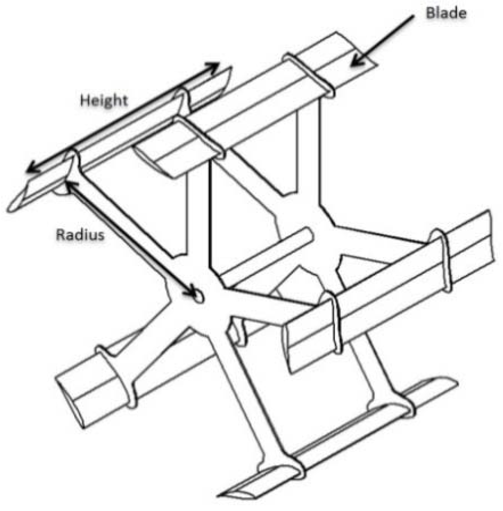
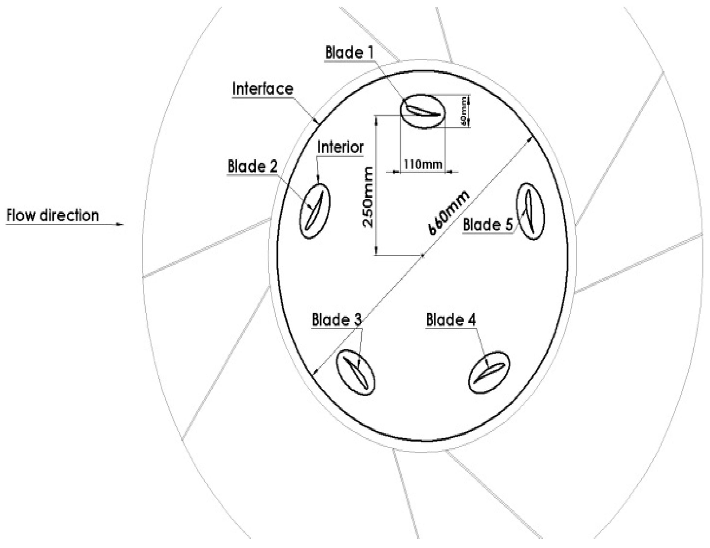
2.1. The VAWT Geometry
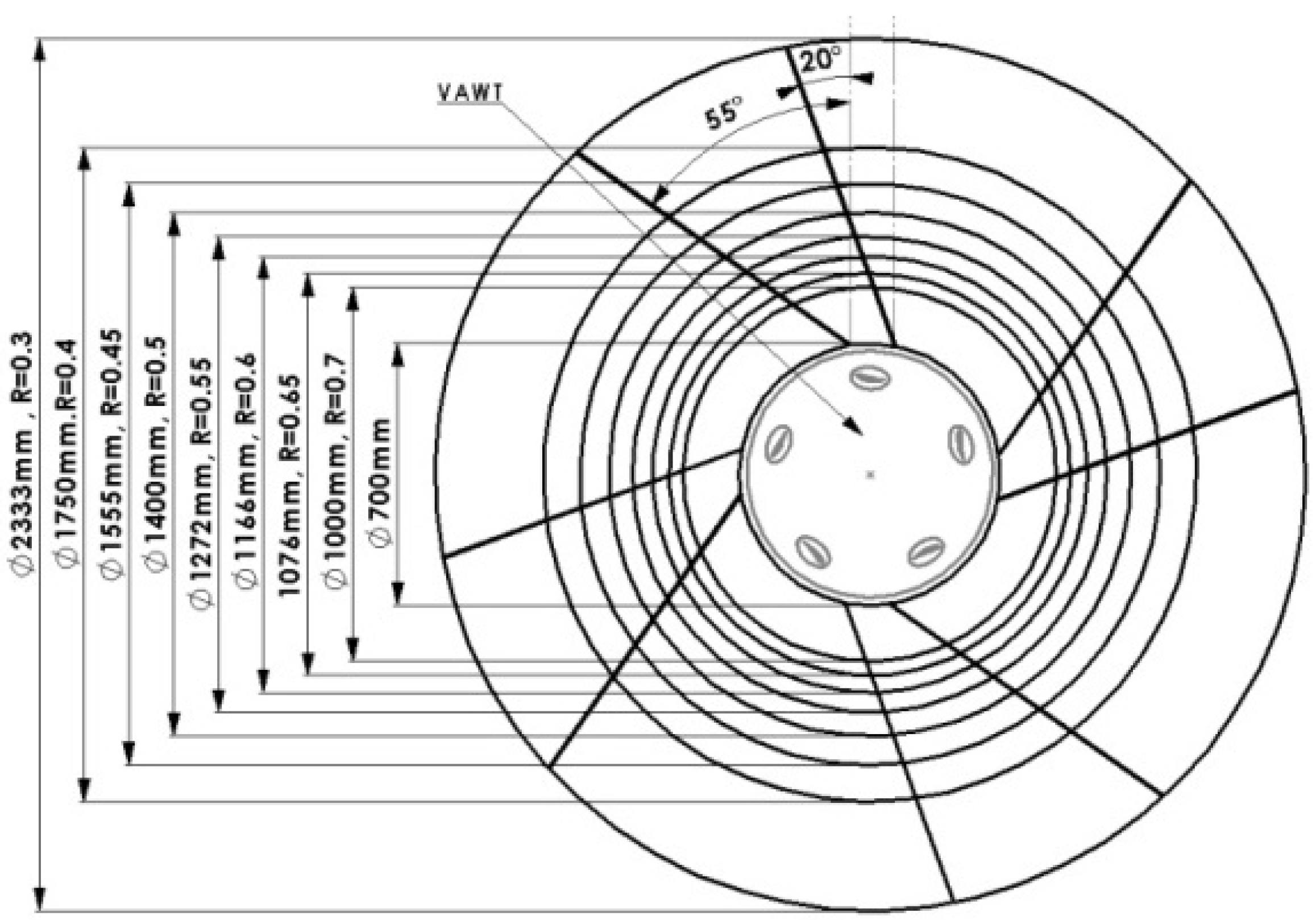
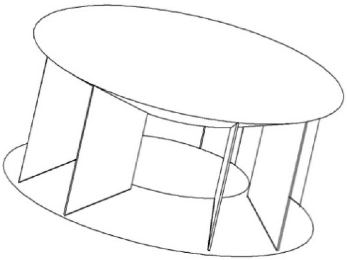
2.2. Geometry of ODGV
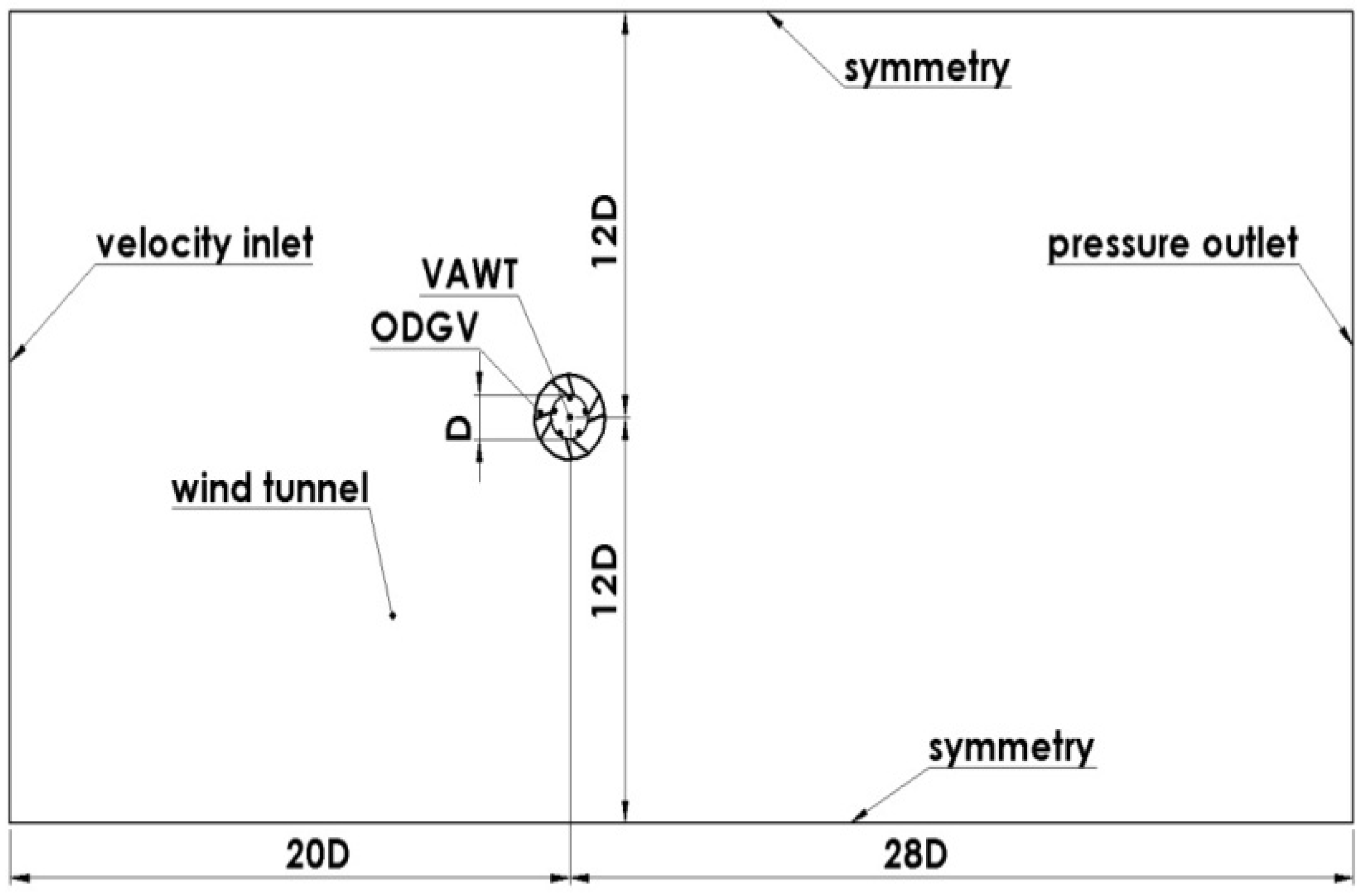
2.3. The Wind Tunnel Numerical Domain
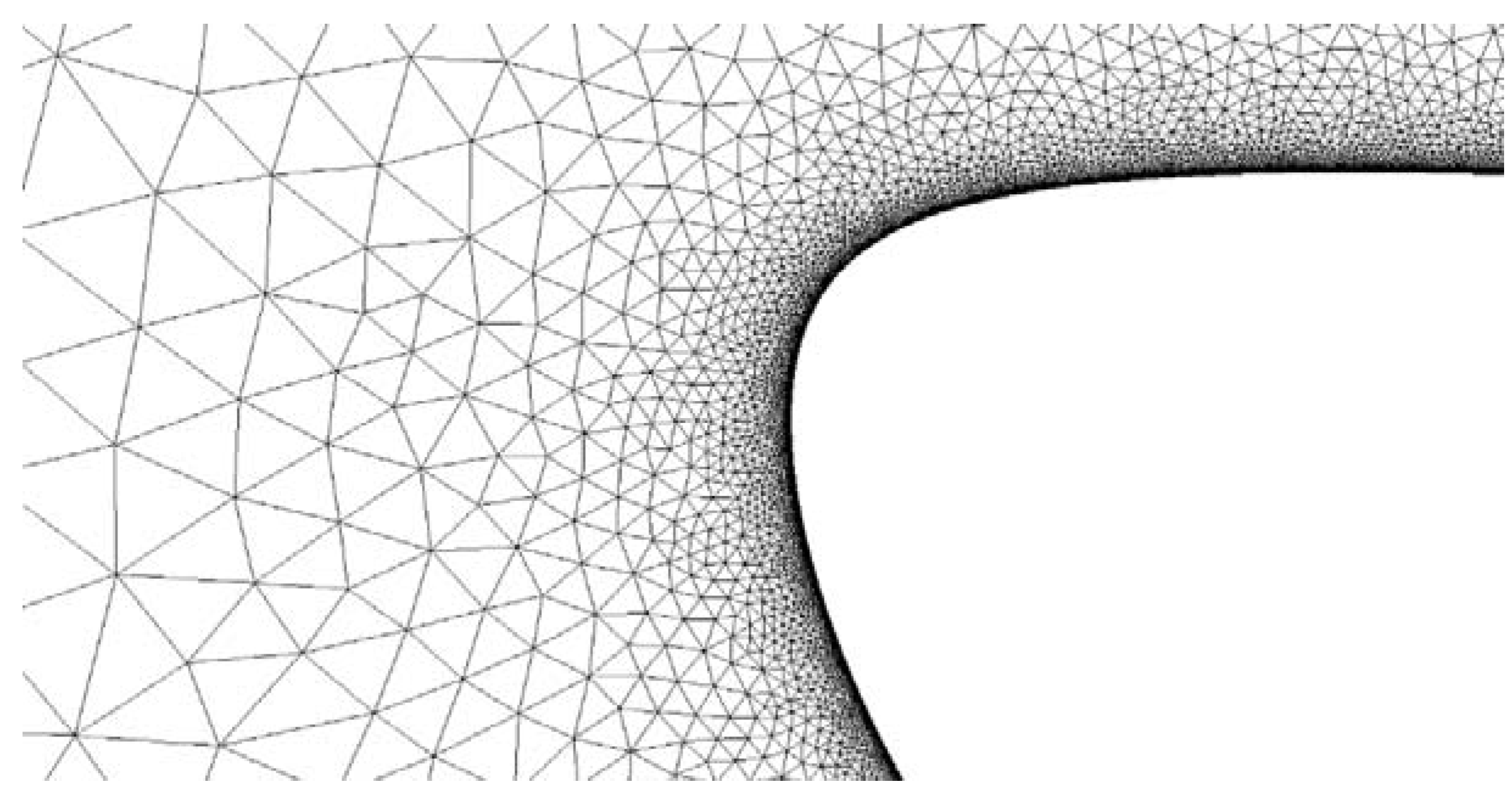
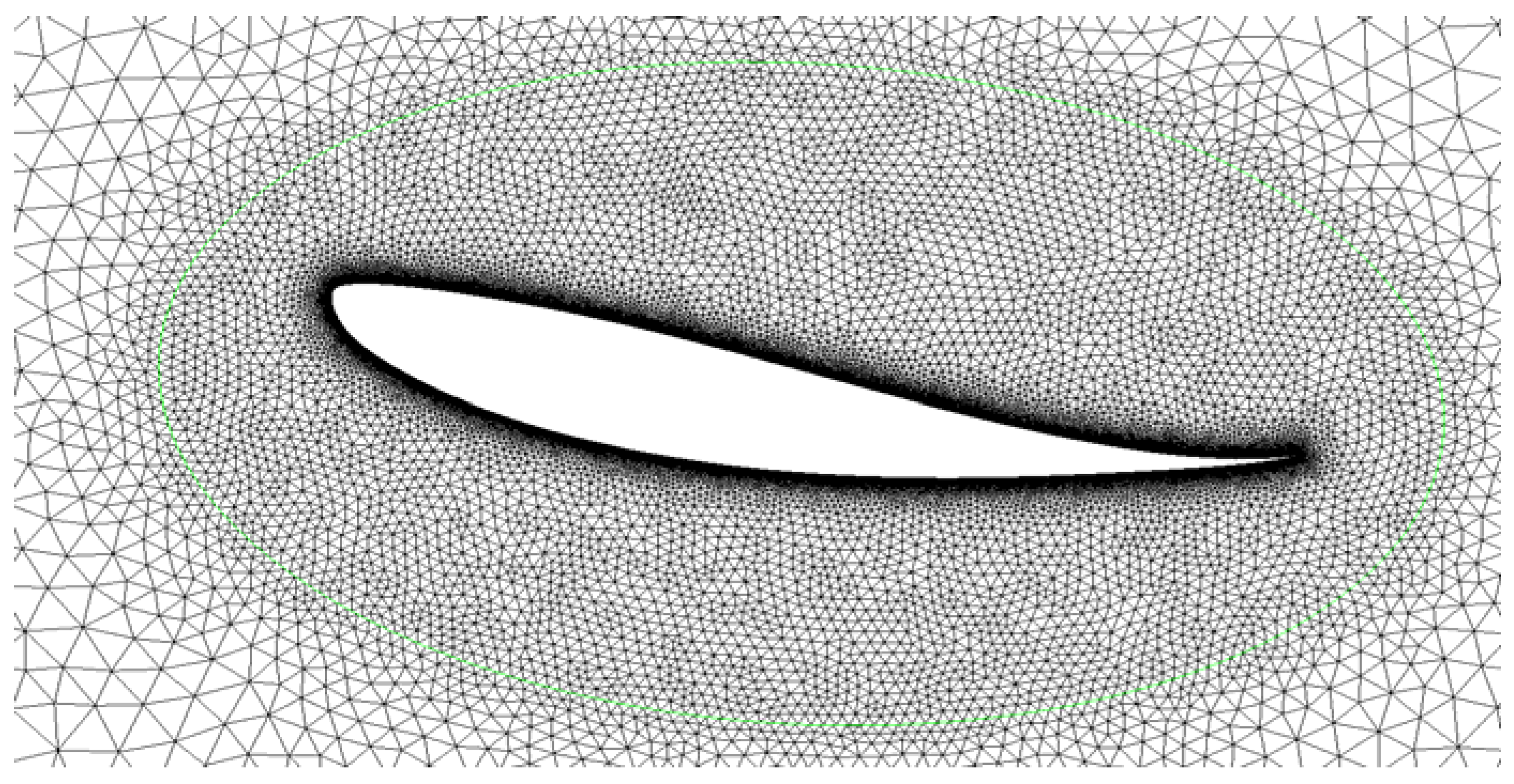
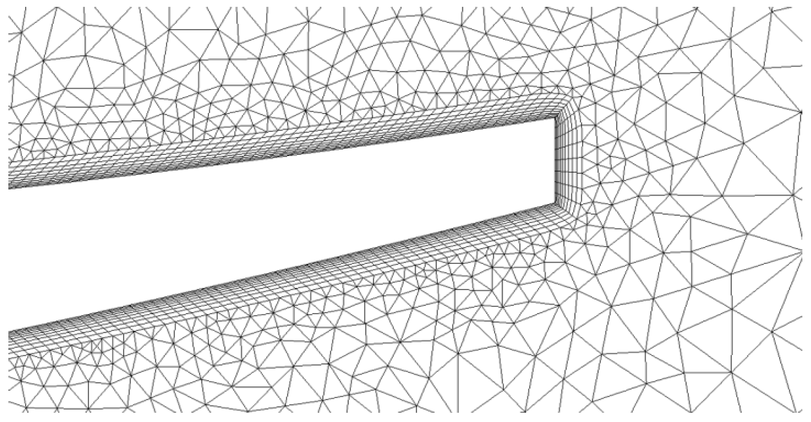
2.4. Mesh Generation and Boundaries
2.5. The Flow Solver and Turbulence Model
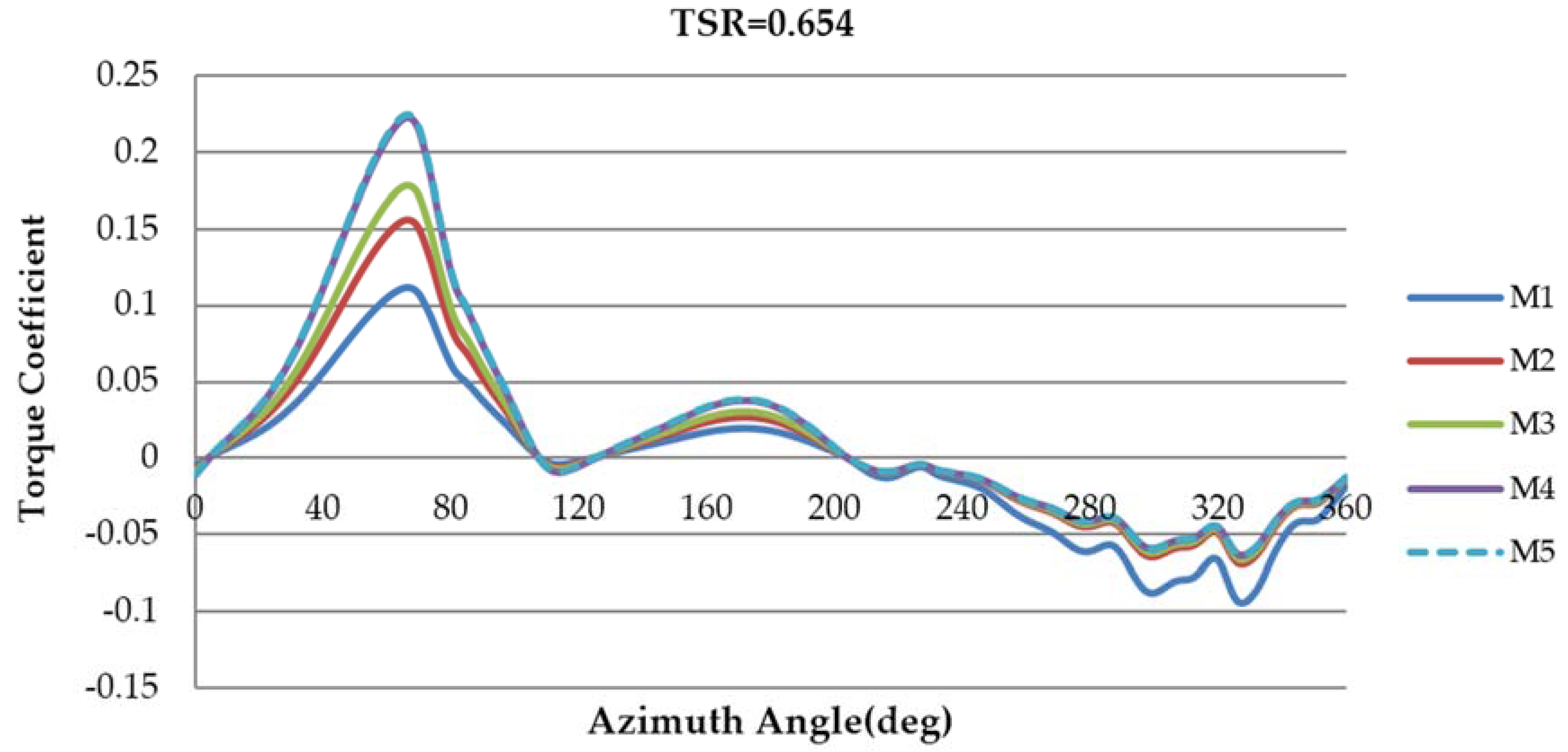
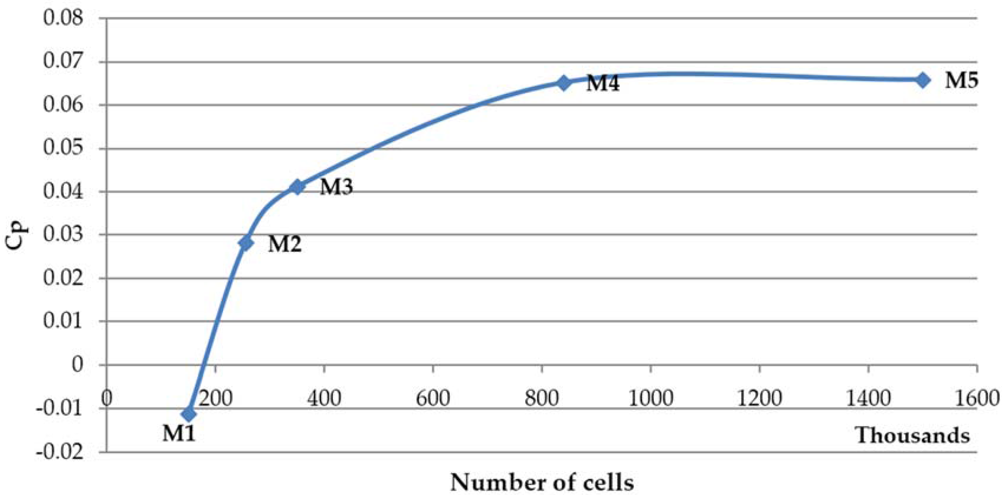
2.6. Mesh Dependency Study
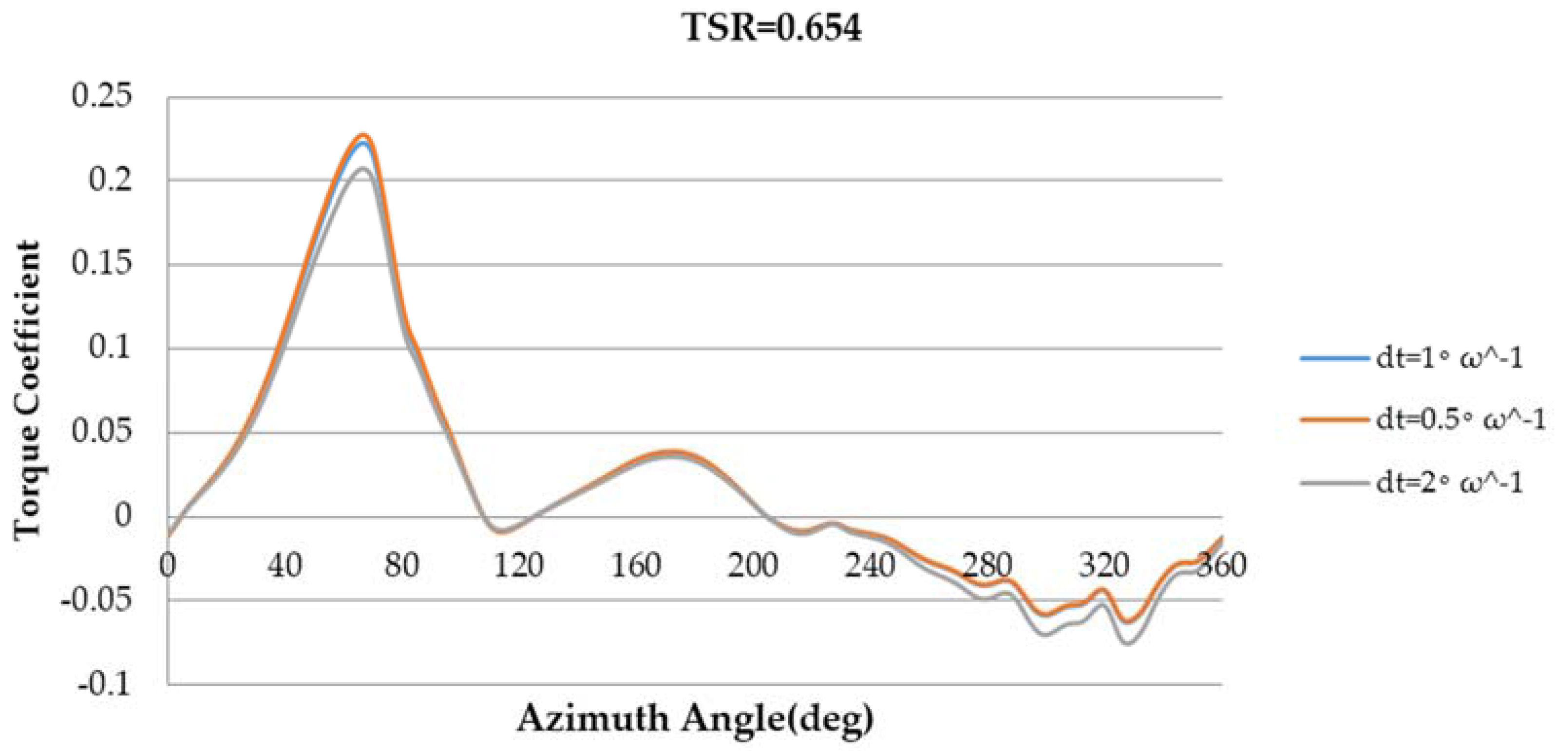
2.7. Time Dependency Study
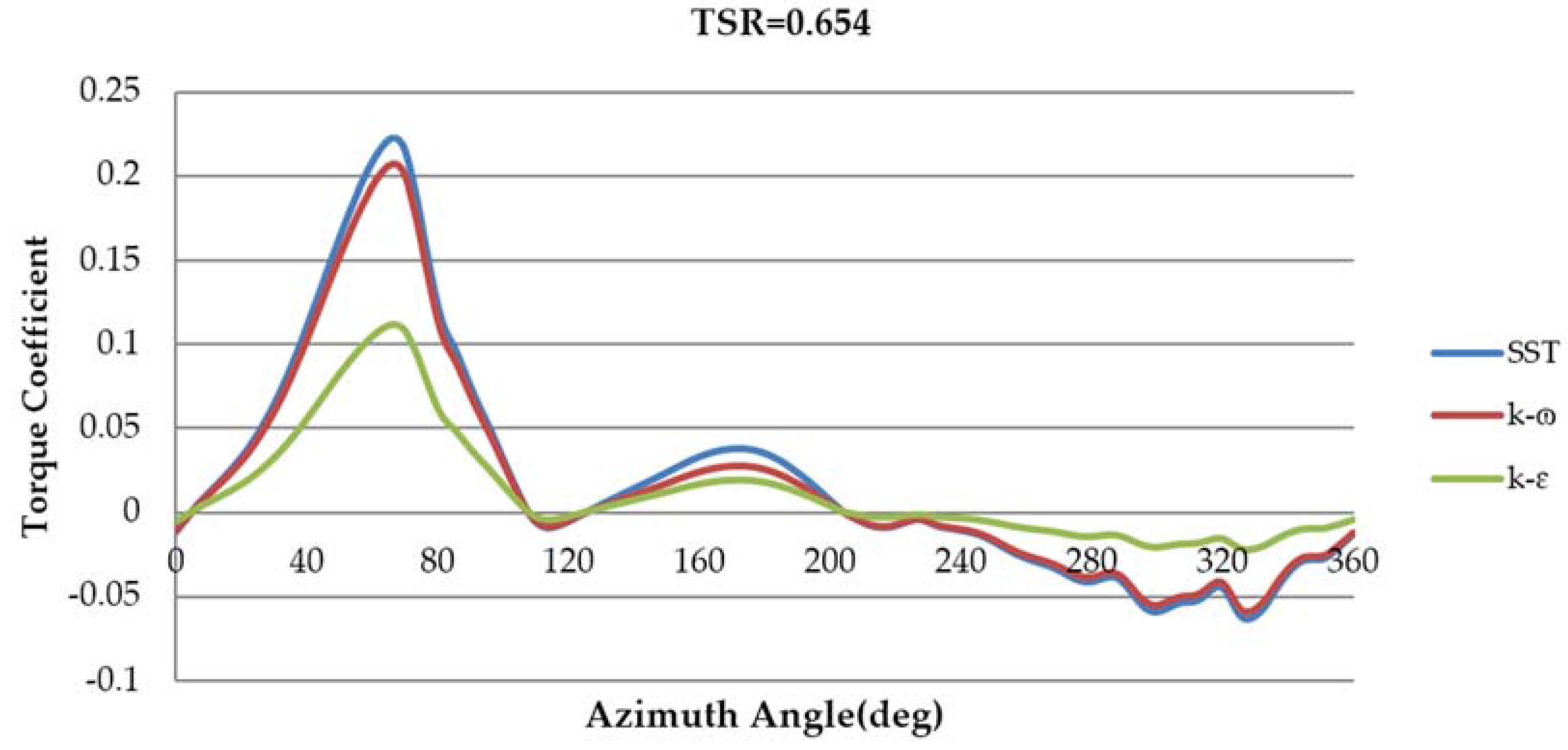
2.8. Turbulence Model Study
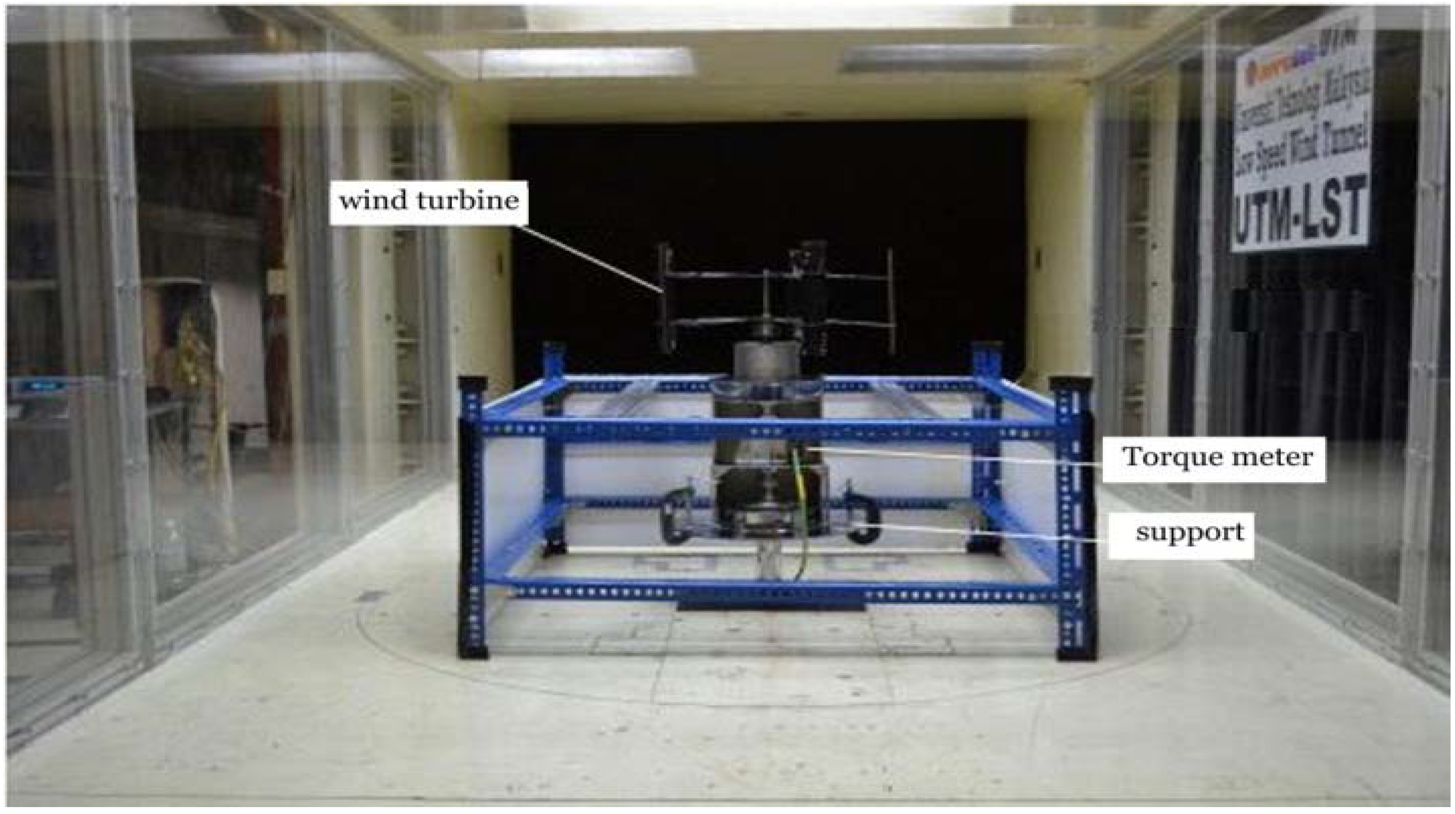
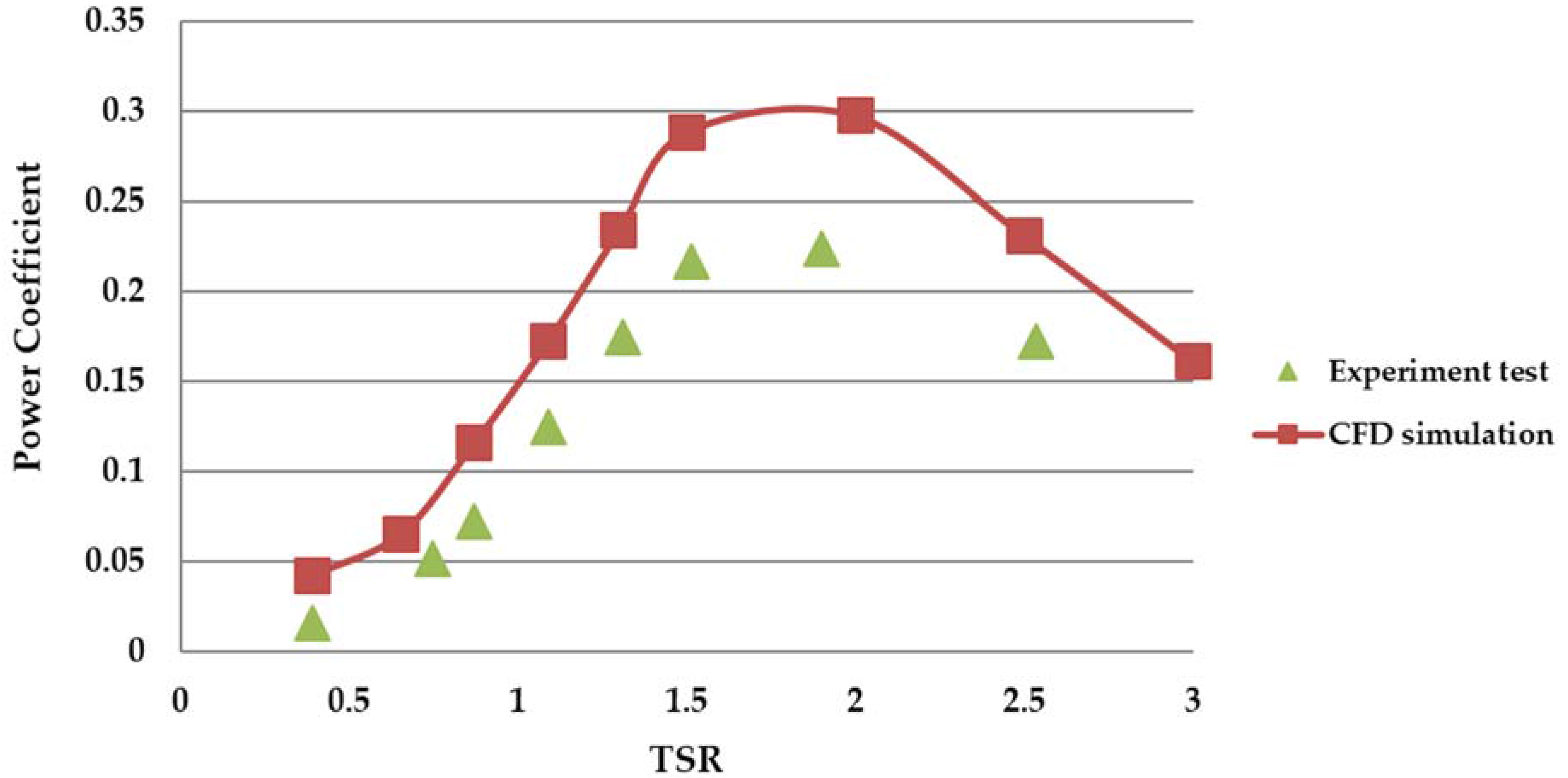
2.9. CFD Validation
3. Results
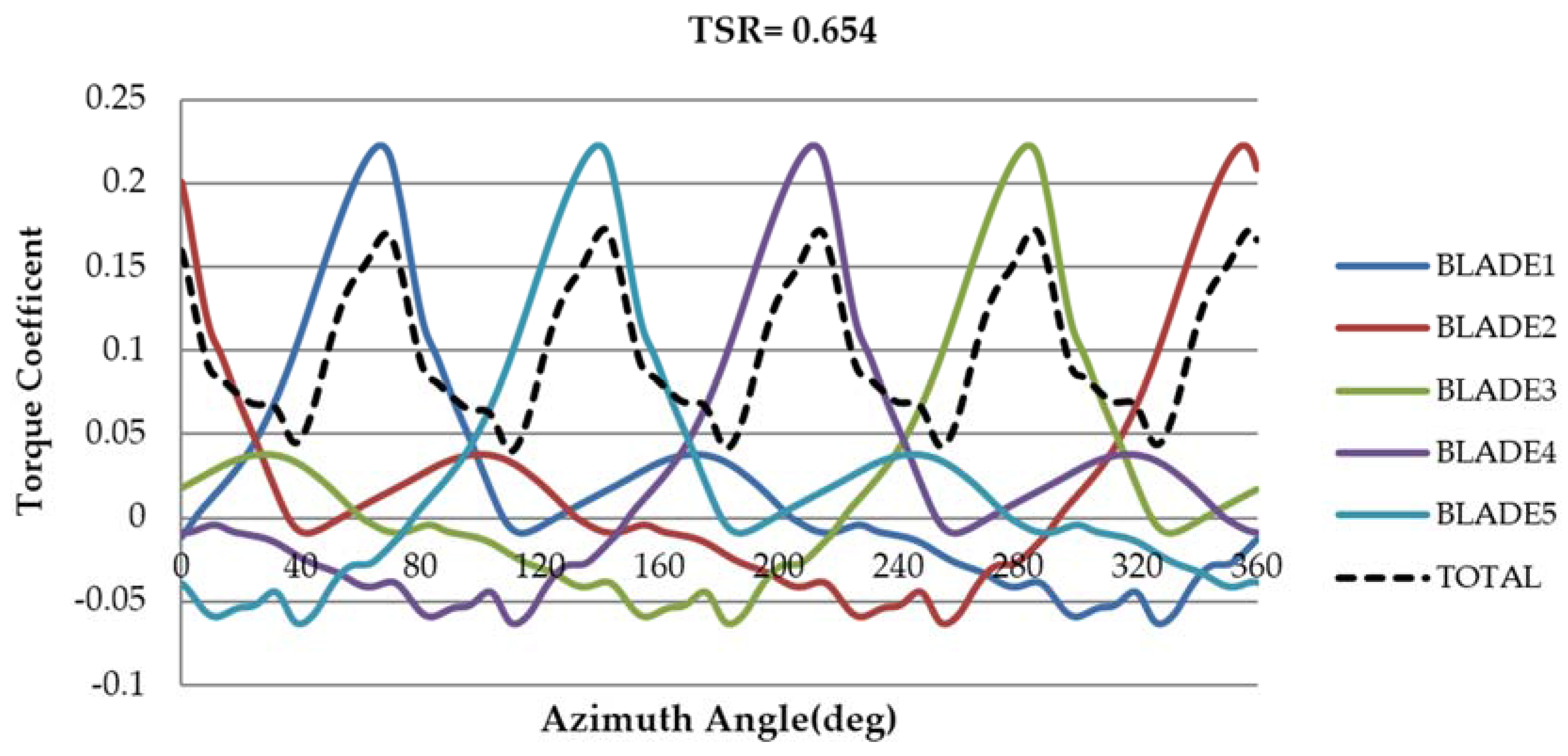
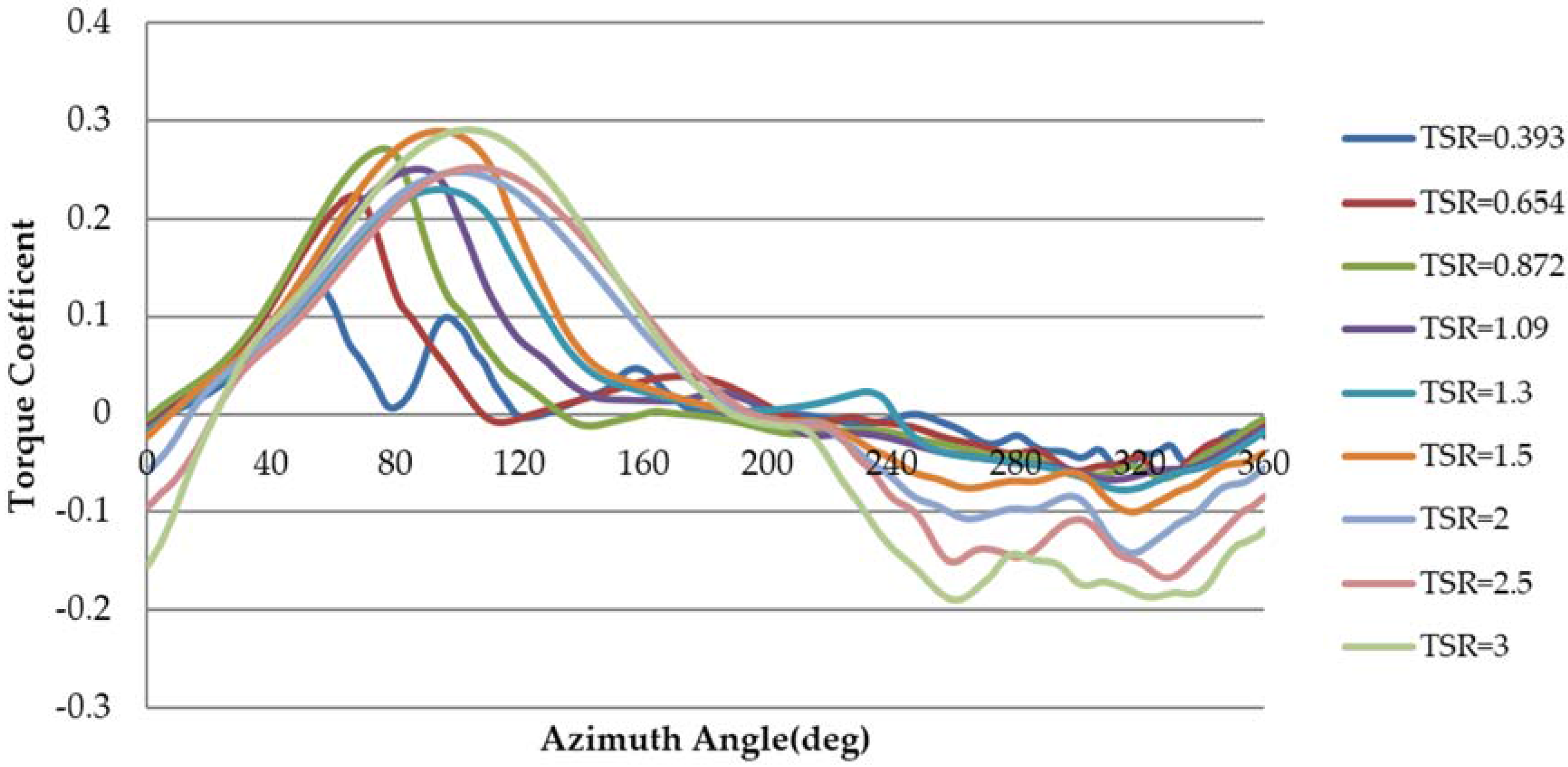
3.1. Case 1: Open Rotor
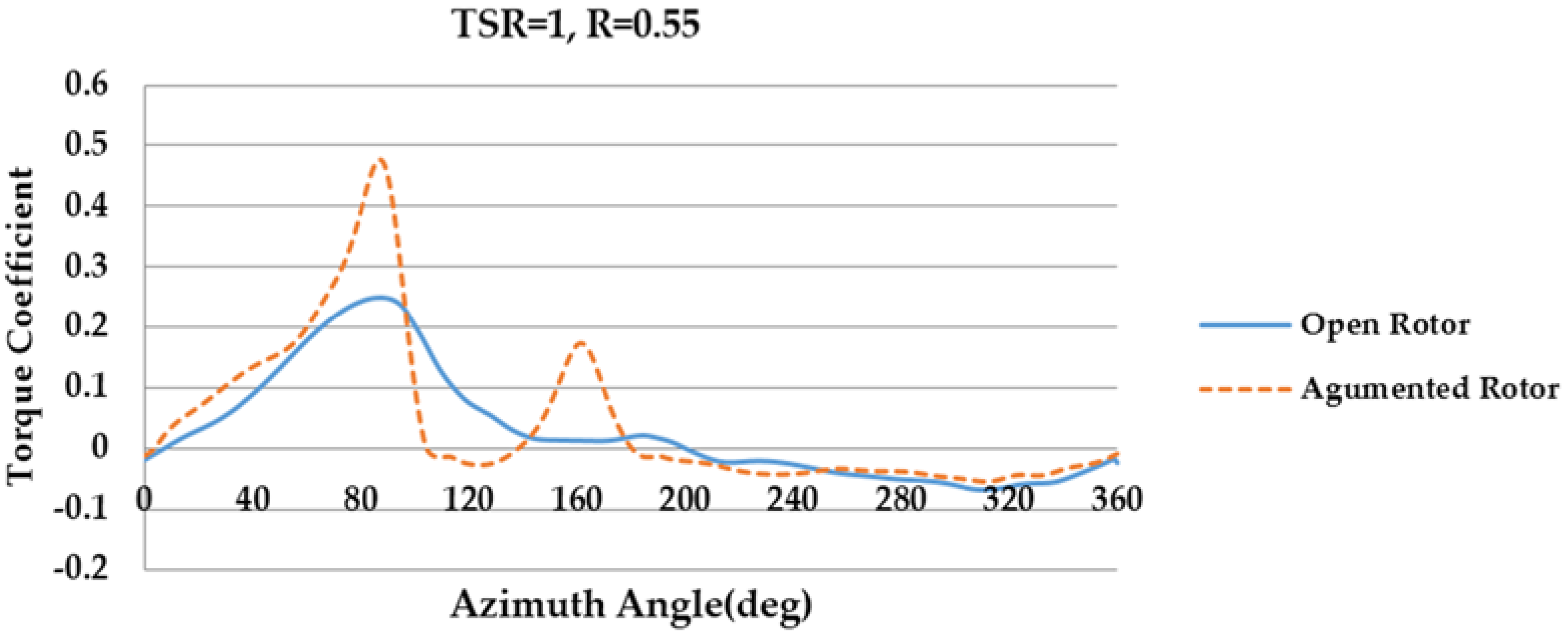
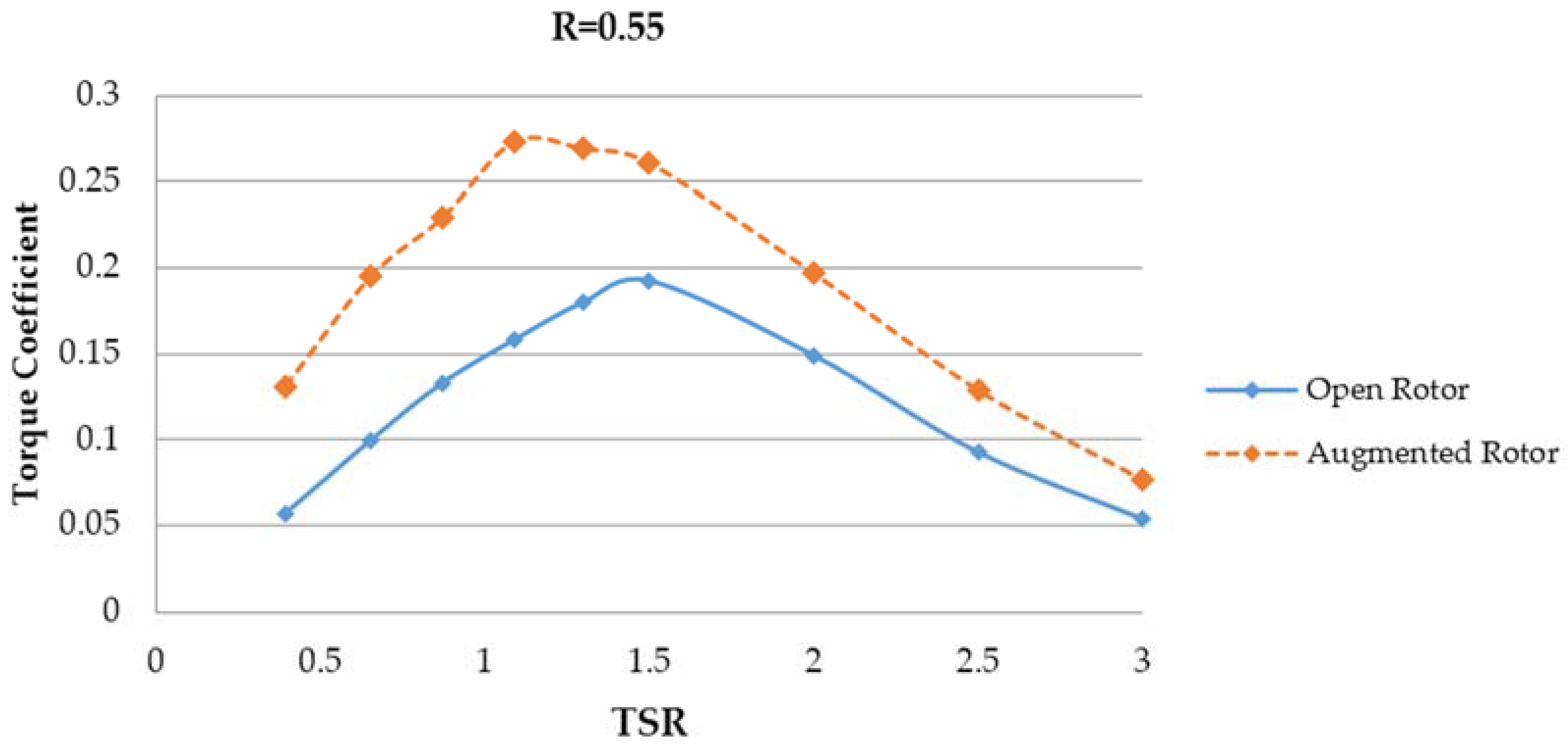
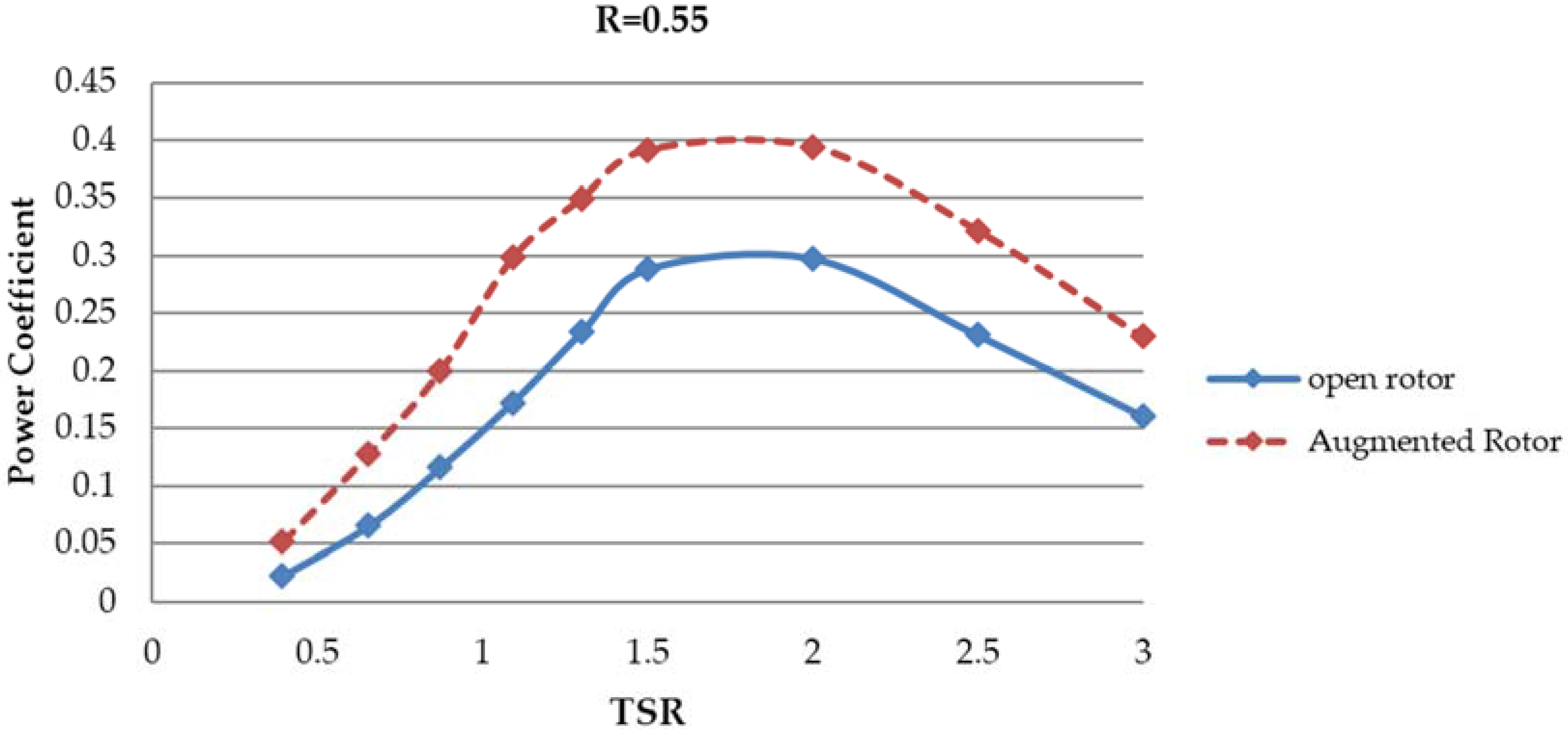
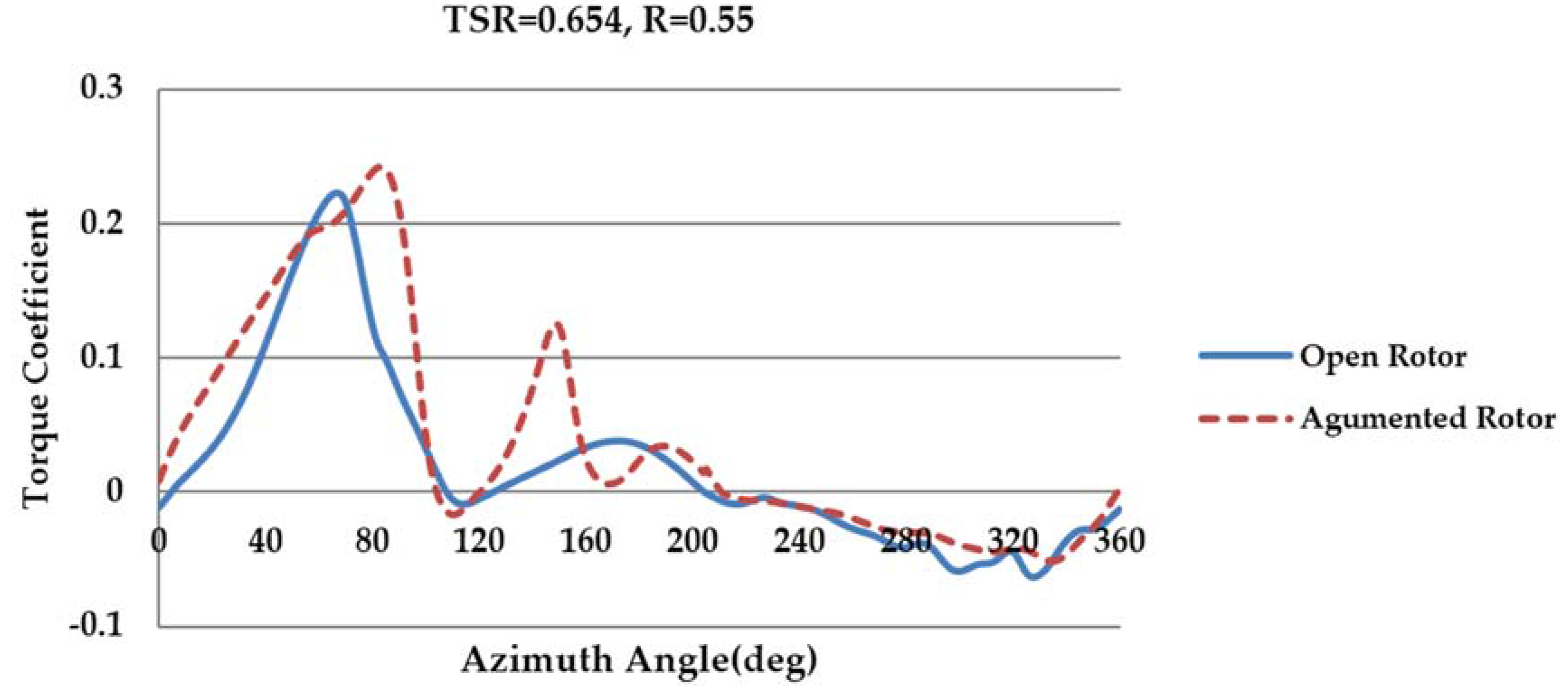
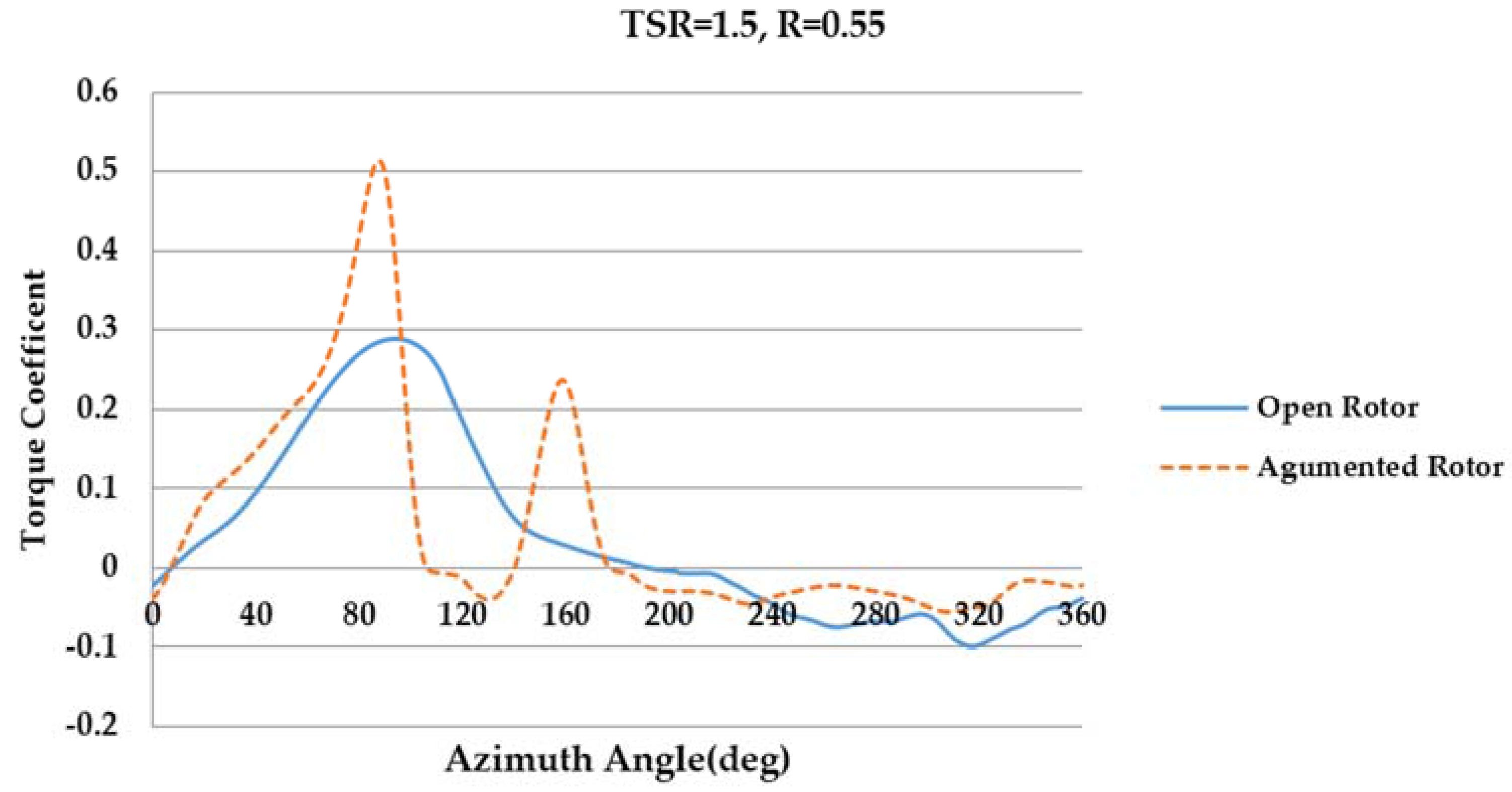
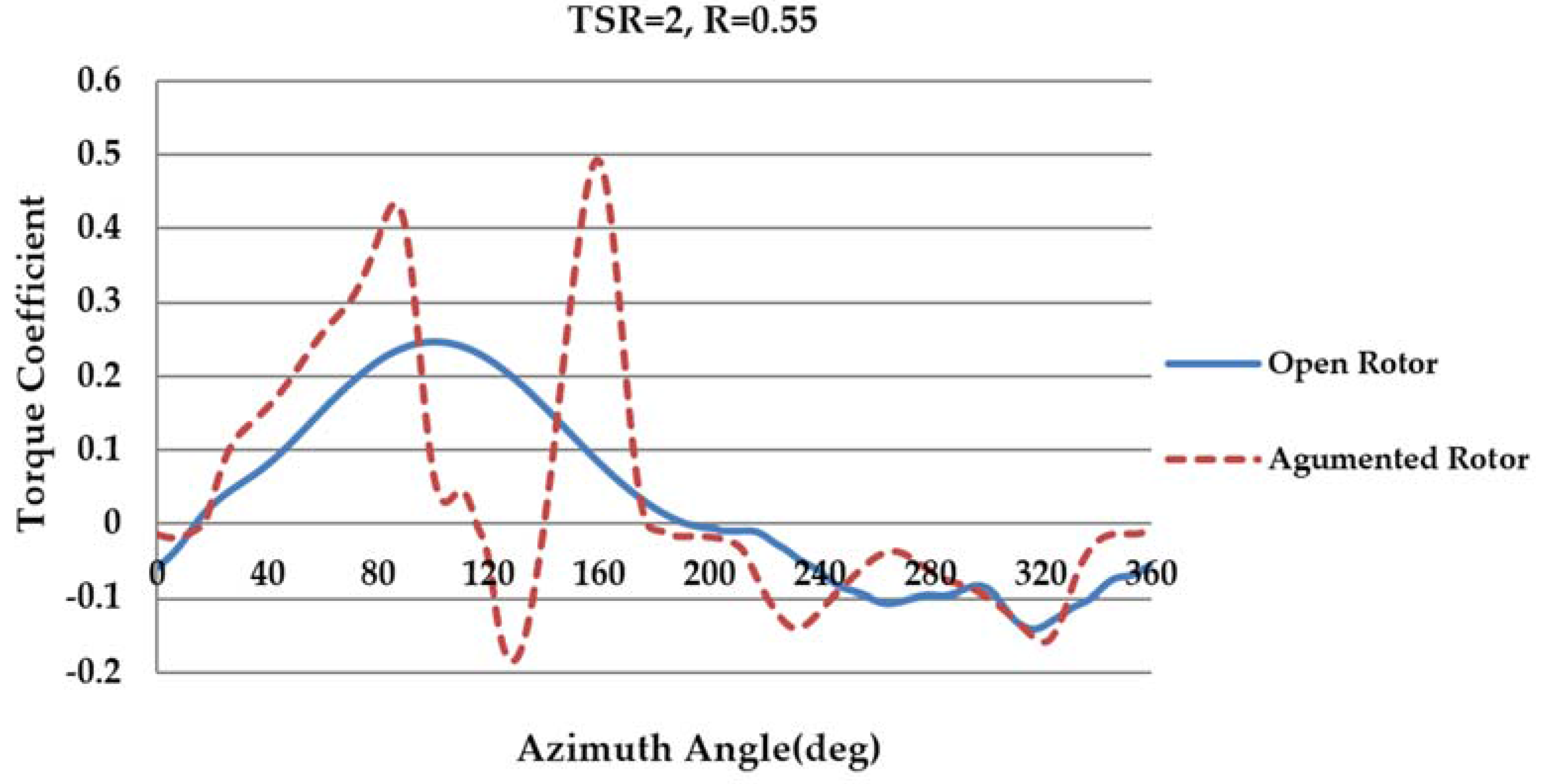
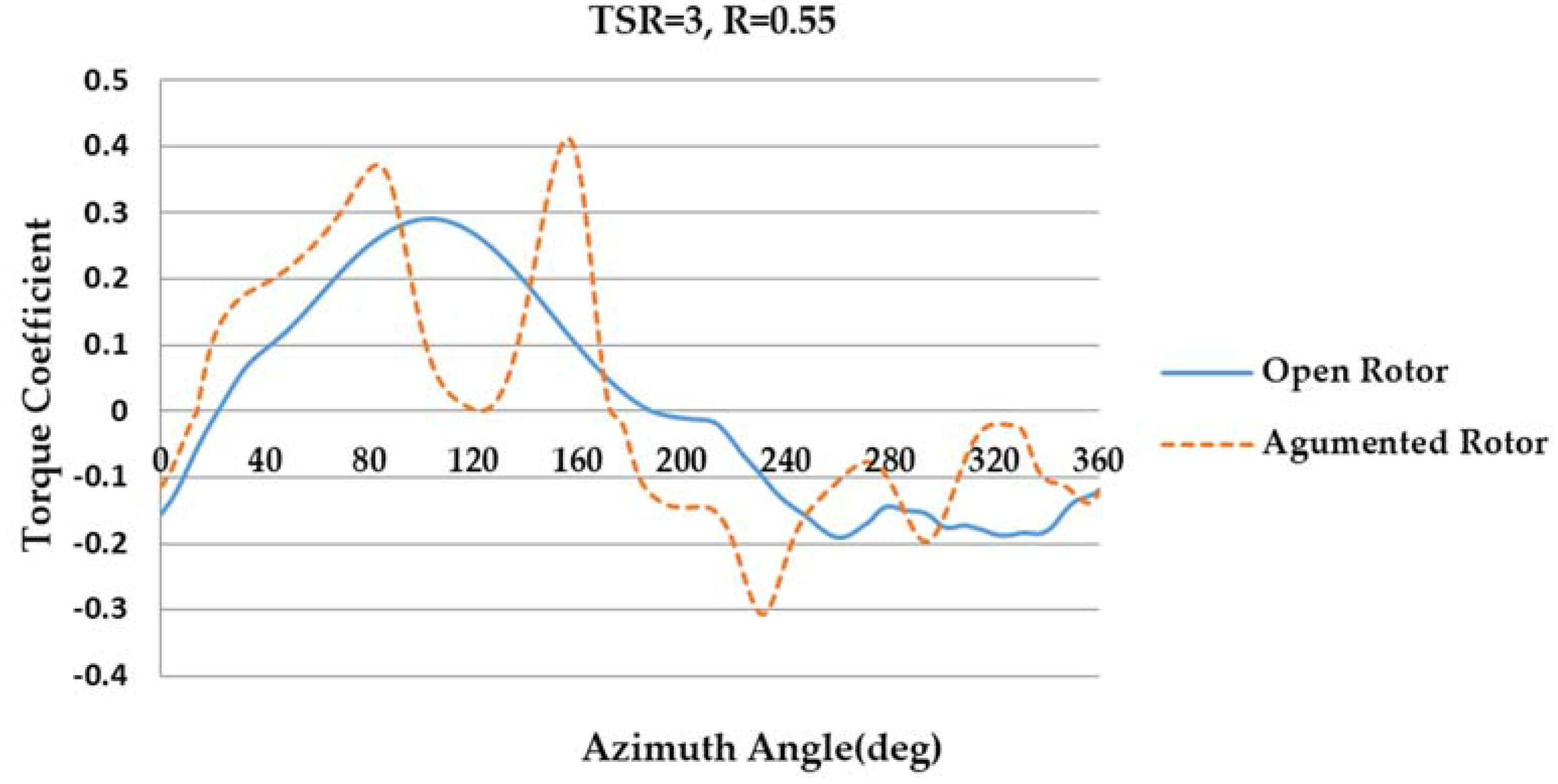
3.2. Case 2: Augmented Rotor and Open Rotor
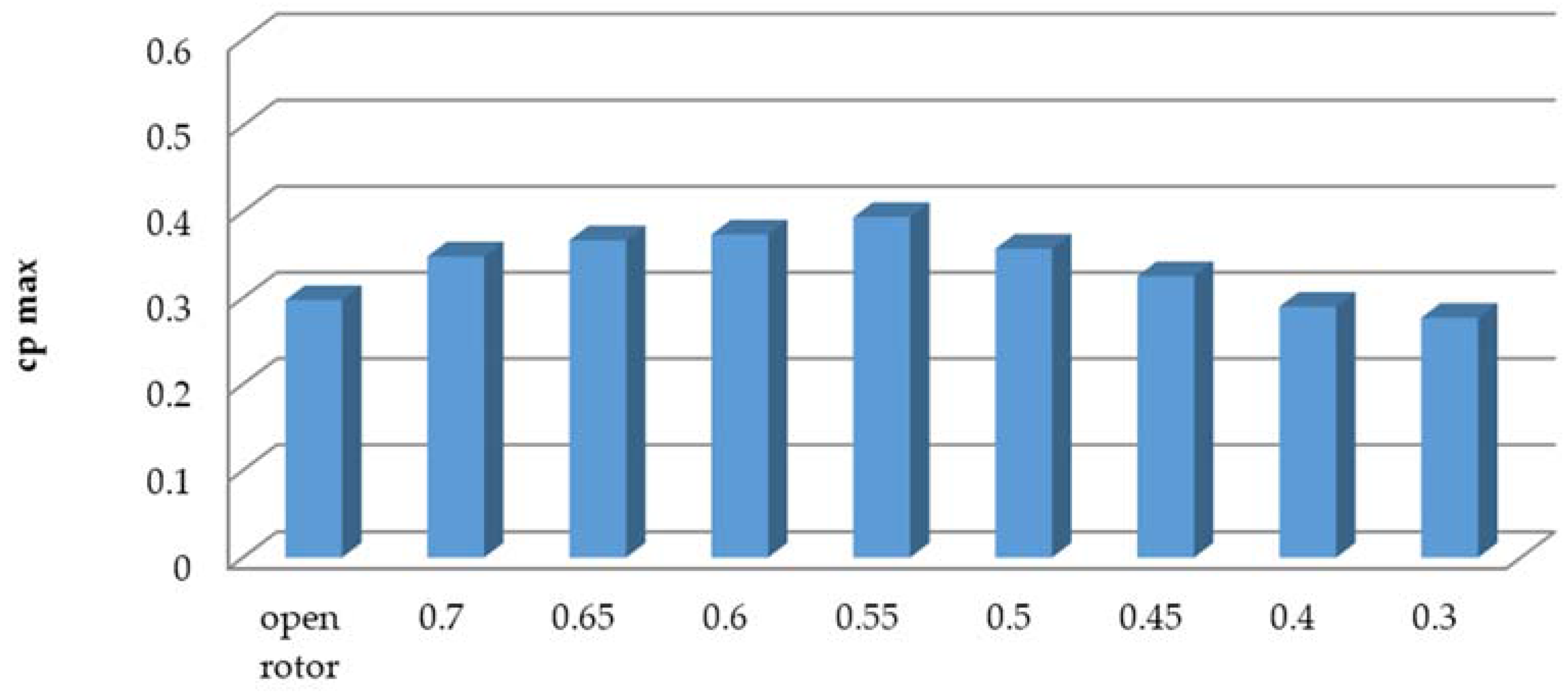
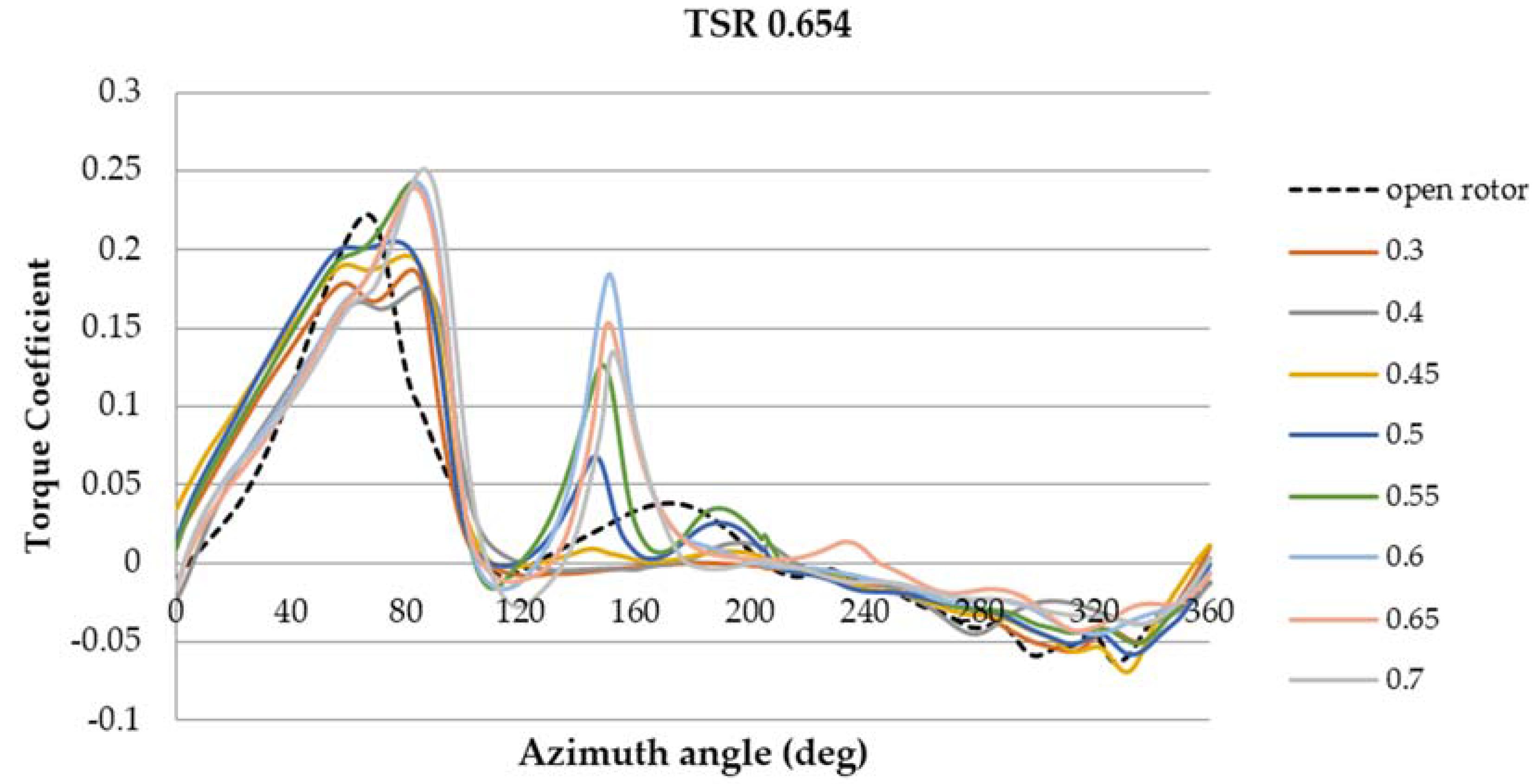
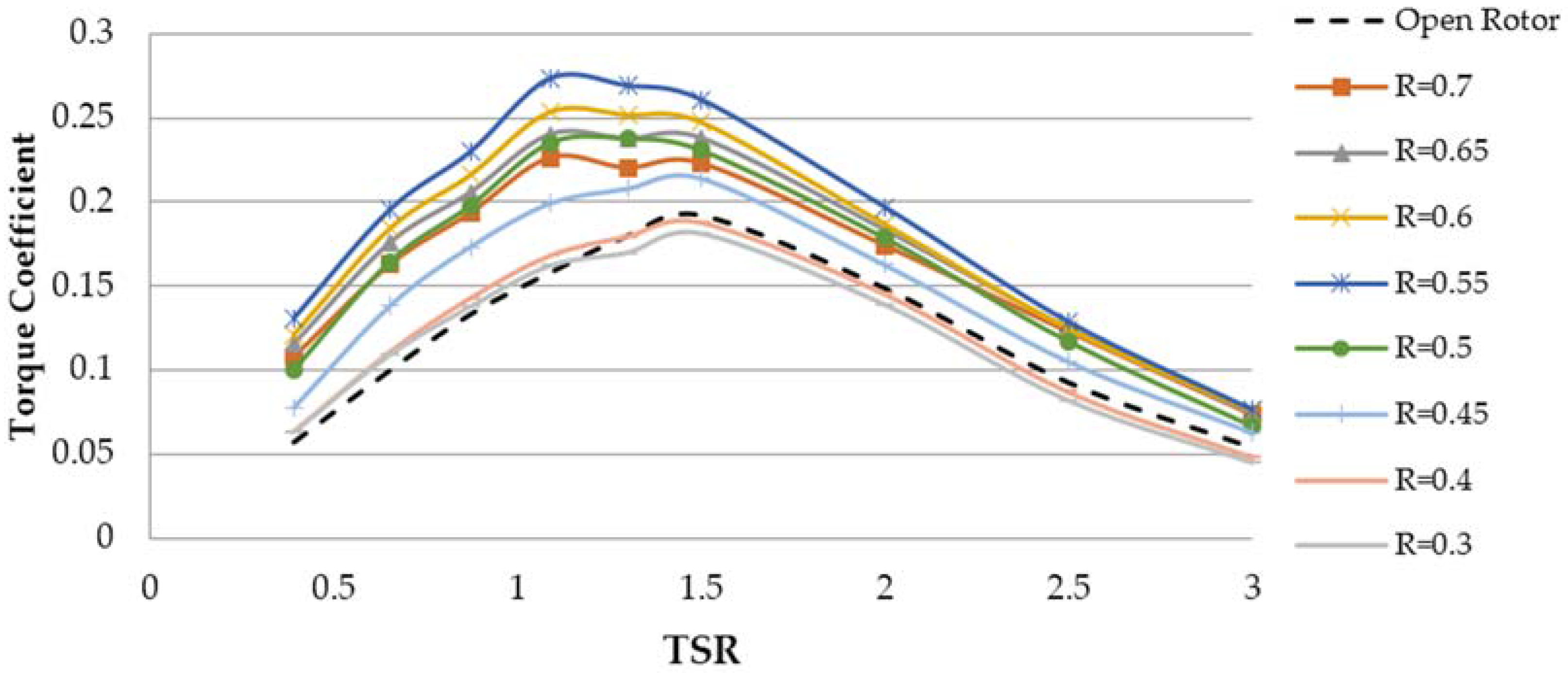
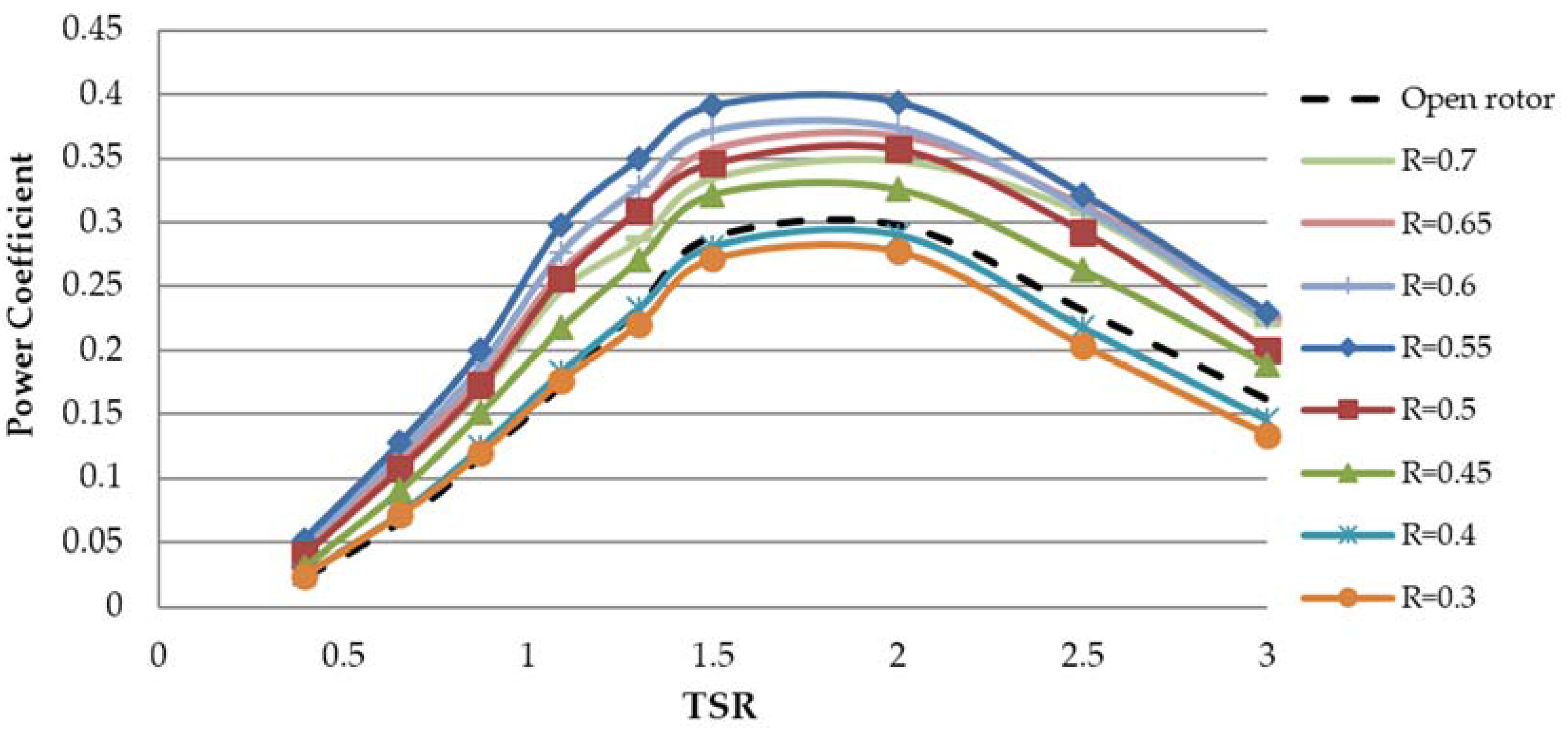
3.3. Case 3: ODGV with Different Shape Ratios
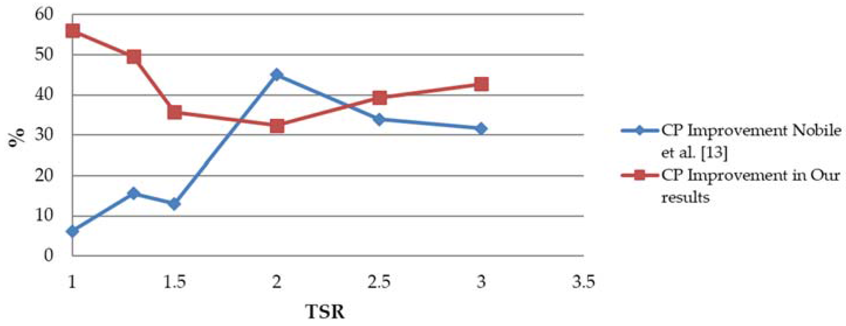
3.4. Comparison with Previous Study Results
4. Discussion
5. Conclusions
Acknowledgments
Author Contributions
Conflicts of Interest
Nomenclature
| Swept turbine area | |
| Blade chord length | |
| CQ | Torque coefficient |
| CQ,ave | Average torque coefficient |
| Average power coefficient | |
| Power coefficient | |
| Turbine diameter | |
| H | Height of the blade |
| HAWT | Horizontal axis wind turbine |
| LES | Large Eddy Simulation |
| N | Number of blades |
| ODGV | omni direction guide vane |
| Rshape-ratio | Shape ratio of the ODGV |
| RANS | Reynolds Averaged Navier Stokes |
| Rrotor | Rotor radius |
| SST | Shear Stress Transport |
| Thickness of the blade | |
| TSR | Tip speed ratio |
| Relative wind speed | |
| VAWT | Vertical axis wind turbine |
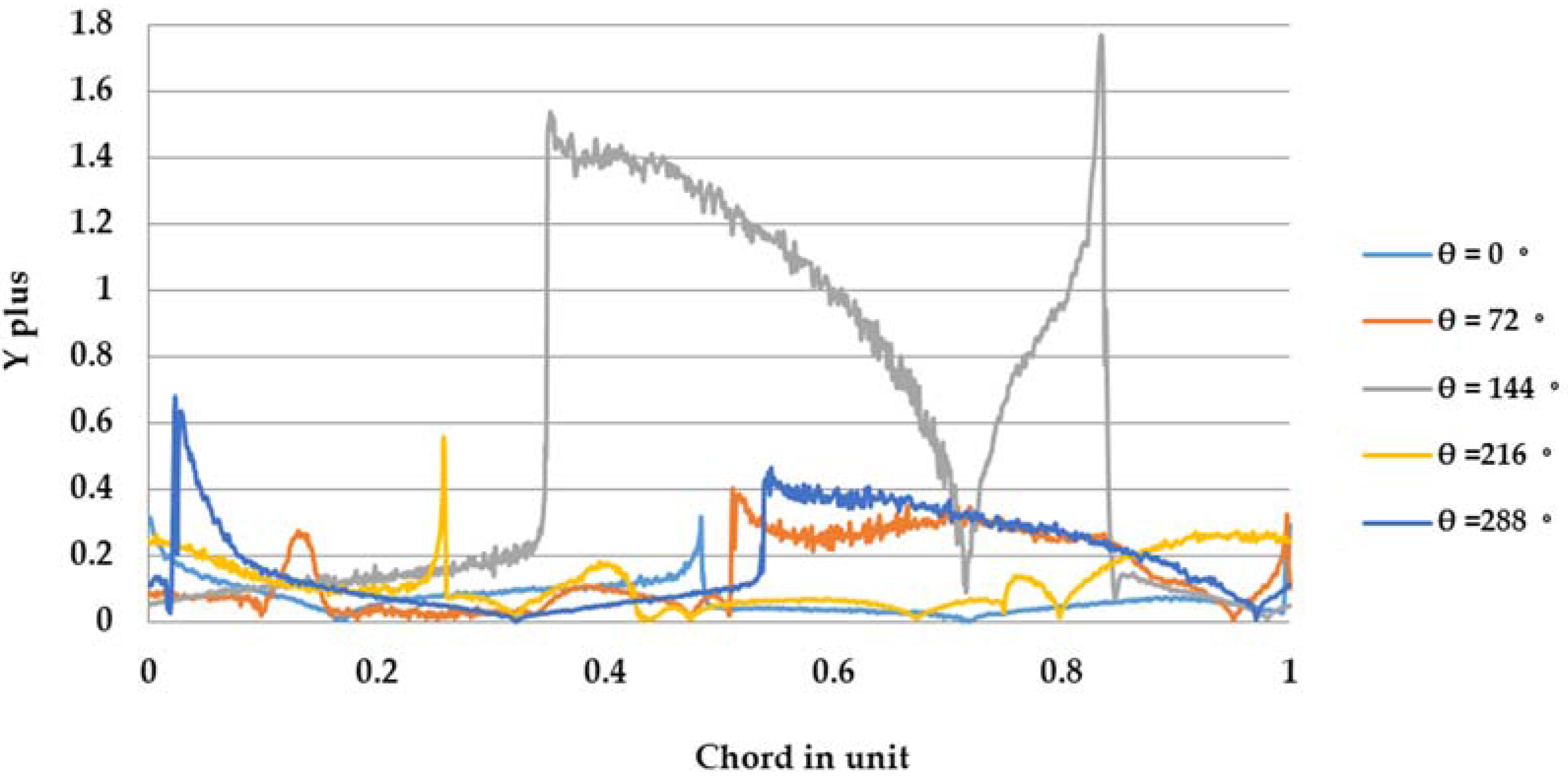
| Yplus | A non-dimensional wall distance for a wall-bounded flow |
| Turbine angular velocity | |
| Azimuth angle |
References
- McLaren, K.W. A Numerical and Experimental Study of Unsteady Loading of High Solidity Vertical Axis Wind Turbines. Ph.D. Thesis, McMaster University, Hamilton, ON, Canada, October 2011. [Google Scholar]
- Gharali, K.; Johnson, D.A. Numerical modeling of an S809 airfoil under dynamic stall, erosion and high reduced frequencies. Appl. Energy 2012, 93, 45–52. [Google Scholar] [CrossRef]
- Hofemann, C.; Simao Ferreira, C.; van Bussel, G.; van Kuik, G.; Scarano, F.; Dixon, K. 3D Stereo PIV study of tip vortex evolution on a vawt. In Proceedings of the European Wind Energy Conference and Exhibition EWEC, Brussels, Belgium, 31 March–3 April 2008; European Wind Energy Association: Bruxelles, Belgium, 2008. [Google Scholar]
- Mertens, S. Wind Energy in the Built Environment: Concentrator Effects of Buildings; Delft University of Technology: Delft, The Netherlands, 2006. [Google Scholar]
- Ferreira, C.S.; van Bussel, G.; van Kuik, G. 2D CFD simulation of dynamic stall on a vertical axis wind turbine: Verification and validation with PIV measurements. In Proceedings of the 45th AIAA Aerospace Sciences Meeting and Exhibit, Reno, NV, USA, 8–11 January 2007; pp. 1–11.
- Chong, W.; Fazlizan, A.; Poh, S.; Pan, K.; Hew, W.; Hsiao, F. The design, simulation and testing of an urban vertical axis wind turbine with the omni-direction-guide-vane. Appl. Energy 2013, 112, 601–609. [Google Scholar] [CrossRef]
- Chong, W.; Fazlizan, A.; Poh, S.; Pan, K.; Ping, H. Early development of an innovative building integrated wind, solar and rain water harvester for urban high rise application. Energy Build. 2012, 47, 201–207. [Google Scholar] [CrossRef]
- Chong, W.; Naghavi, M.; Poh, S.; Mahlia, T.; Pan, K. Techno-economic analysis of a wind-solar hybrid renewable energy system with rainwater collection feature for urban high-rise application. Appl. Energy 2011, 88, 4067–4077. [Google Scholar] [CrossRef]
- Chong, W.T.; Pan, K.C.; Poh, S.C.; Fazlizan, A.; Oon, C.S.; Badarudin, A.; Nik-Ghazali, N. Performance investigation of a power augmented vertical axis wind turbine for urban high-rise application. Renew. Energy 2013, 51, 388–397. [Google Scholar] [CrossRef]
- Oman, R.; Foreman, K.; Gilbert, B.L. Investigation of Diffuser-Augmented Wind Turbines; Progress Report; Grumman Aerospace Corp.: Bethpage, NY, USA, 1976; p. 1. [Google Scholar]
- Thomas, R.N. Vertical Windmill with Omnidirectional Diffusion. US Patent 5332925, 26 July 1994. [Google Scholar]
- Wang, Y.F.; Zhan, M.S. Effect of barchan dune guide blades on the performance of a lotus-shaped micro-wind turbine. J. Wind Eng. Ind. Aerodyn. 2015, 136, 34–43. [Google Scholar] [CrossRef]
- Nobile, R.; Vahdati, M.; Barlow, J.F.; Mewburn-Crook, A. Unsteady flow simulation of a vertical axis augmented wind turbine: A two-dimensional study. J. Wind Eng. Ind. Aerodyn. 2014, 125, 168–179. [Google Scholar] [CrossRef]
- Danao, L.A.; Edwards, J.; Eboibi, O.; Howell, R. A numerical investigation into the influence of unsteady wind on the performance and aerodynamics of a vertical axis wind turbine. Appl. Energy 2014, 116, 111–124. [Google Scholar] [CrossRef]
- Almohammadi, K.M.; Ingham, D.B.; Ma, L.; Pourkashan, M. Computational fluid dynamics (CFD) mesh independency techniques for a straight blade vertical axis wind turbine. Energy 2013, 58, 483–493. [Google Scholar] [CrossRef]
- Pope, K.; Rodrigues, V.; Doyle, R.; Tsopelas, A.; Gravelsins, R.; Naterer, G.F.; Tsang, E. Effects of stator vanes on power coefficients of a zephyr vertical axis wind turbine. Renew. Energy 2010, 35, 1043–1051. [Google Scholar] [CrossRef]
- Takao, M.; Kuma, H.; Maeda, T.; Kamada, Y.; Oki, M.; Minoda, A. A straight-bladed vertical axis wind turbine with a directed guide vane row—Effect of guide vane geometry on the performance. J. Therm. Sci. 2009, 18, 54–57. [Google Scholar] [CrossRef]
- Edwards, J.M.; Danao, L.A.; Howell, R.J. Novel experimental power curve determination and computational methods for the performance analysis of vertical axis wind turbines. J. Sol. Energy Eng. 2012, 134, 031008. [Google Scholar] [CrossRef]
- Danao, L.A.; Howell, R. Effects on the performance of vertical axis wind turbines with unsteady wind inflow: A numerical study. In Proceedings of the 50th AIAA Aerospace Sciences Meeting Including the New Horizons Forum and Aerospace Exposition, Nashville, TN, USA, 9–12 January 2012.
- Amet, E.; MaÃŽtre, T.; Pellone, C.; Achard, J.L. 2D numerical simulations of blade-vortex interaction in a Darrieus turbine. J. Fluids Eng. 2009, 131, 111103. [Google Scholar] [CrossRef]
- Aslam Bhutta, M.M.; Hayat, N.; Farooq, A.U.; Ali, Z.; Jamil, S.R.; Hussain, Z. Vertical axis wind turbine—A review of various configurations and design techniques. Renew. Sustain. Energy Rev. 2012, 16, 1926–1939. [Google Scholar] [CrossRef]
- Balduzzi, F.; Bianchini, A.; Carnevale, E.A.; Ferrari, L.; Magnani, S. Feasibility analysis of a Darrieus vertical-axis wind turbine installation in the rooftop of a building. Appl. Energy 2012, 97, 921–929. [Google Scholar] [CrossRef]
- Kang, C.; Liu, H.; Yang, X. Review of fluid dynamics aspects of Savonius-rotor-based vertical-axis wind rotors. Renew. Sustain. Energy Rev. 2014, 33, 499–508. [Google Scholar] [CrossRef]
- Wekesa, D.W.; Wang, C.; Wei, Y.; Danao, L.A.M. Influence of operating conditions on unsteady wind performance of vertical axis wind turbines operating within a fluctuating free-stream: A numerical study. J. Wind Eng. Ind. Aerodyn. 2014, 135, 76–89. [Google Scholar] [CrossRef]
- Shi, L.; Riziotis, V.; Voutsinas, S.; Wang, J. A consistent vortex model for the aerodynamic analysis of vertical axis wind turbines. J. Wind Eng. Ind. Aerodyn. 2014, 135, 57–69. [Google Scholar] [CrossRef]
- Alaimo, A.; Esposito, A.; Messineo, A.; Orlando, C.; Tumino, D. 3D CFD Analysis of a Vertical Axis Wind Turbine. Energies 2015, 8, 3013–3033. [Google Scholar] [CrossRef]
- Hasan, M.R.; Islam, M.R.; Hasan Shahariar, G.; Mashud, M. Numerical analysis of vertical axis wind turbine. In Proceedings of the IEEE 9th International Forum on Strategic Technology, Cox’s Bazar, Bangladesh, 21–23 October 2014; pp. 318–321.
- Howell, R.; Qin, N.; Edwards, J.; Durrani, N. Wind tunnel and numerical study of a small vertical axis wind turbine. Renew. Energy 2010, 35, 412–422. [Google Scholar] [CrossRef]
- De Marco, A.; Coiro, D.P.; Cucco, D.; Nicolosi, F. A Numerical Study on a Vertical-Axis Wind Turbine with Inclined Arms. Int. J. Aerosp. Eng. 2014, 2014. [Google Scholar] [CrossRef]
- Coiro, D.; Nicolosi, F.; de Marco, A.; Melone, S.; Montella, F. Flow Curvature Effect on Dynamic Behaviour of a Novel Vertical Axis Tidal Current Turbine: Numerical and Experimental Analysis. In Proceedings of the ASME 24th International Conference on Offshore Mechanics and Arctic Engineering, Halkidiki, Greece, 12–17 June 2005; American Society of Mechanical Engineers: New York, NY, USA, 2005; pp. 601–609. [Google Scholar]
- Paillard, B.; Astolfi, J.A.; Hauville, F. URANSE simulation of an active variable-pitch cross-flow Darrieus tidal turbine: Sinusoidal pitch function investigation. Int. J. Mar. Energy 2015, 11, 9–26. [Google Scholar] [CrossRef]
- Fluent, A. 12.0 Theory Guide; Ansys Inc.: Cecil Township, PA, USA, 2009; p. 5. [Google Scholar]
- Mohamed, M.H.; Ali, A.M.; Hafiz, A.A. CFD analysis for H-rotor Darrieus turbine as a low speed wind energy converter. Eng. Sci. Technol. Int. J. 2015, 18, 1–13. [Google Scholar] [CrossRef]
- Pope, A.; Harper, J.J. Low Speed Wind Tunnel Testing; John Wiley & Sons: New York, NY, USA, 1966. [Google Scholar]
- Wang, S.; Ingham, D.B.; Ma, L.; Pourkashanian, M.; Tao, Z. Numerical investigations on dynamic stall of low Reynolds number flow around oscillating airfoils. Comput. Fluids 2010, 39, 1529–1541. [Google Scholar] [CrossRef]
- McLaren, K.; Tullis, S.; Ziada, S. Computational fluid dynamics simulation of the aerodynamics of a high solidity, small-scale vertical axis wind turbine. Wind Energy 2012, 15, 349–361. [Google Scholar] [CrossRef]
- Raciti Castelli, M.; Englaro, A.; Benini, E. The Darrieus wind turbine: Proposal for a new performance prediction model based on CFD. Energy 2011, 36, 4919–4934. [Google Scholar] [CrossRef]
- Chen, C.C.; Kuo, C.H. Effects of pitch angle and blade camber on flow characteristics and performance of small-size Darrieus VAWT. J. Vis. 2013, 16, 65–74. [Google Scholar] [CrossRef]
- Guerri, O.; Sakout, A.; Bouhadef, K. Simulations of the fluid flow around a rotating vertical axis wind turbine. Wind Eng. 2007, 31, 149–163. [Google Scholar] [CrossRef]
- Dai, Y.; Lam, W. Numerical study of straight-bladed Darrieus-type tidal turbine. Proc. ICE Energy 2009, 162, 67–76. [Google Scholar] [CrossRef]
- Gupta, R.; Biswas, A. Computational fluid dynamics analysis of a twisted three-bladed H-Darrieus rotor. J. Renew. Sustain. Energy 2010, 2, 043111. [Google Scholar] [CrossRef]
- Maître, T.; Amet, E.; Pellone, C. Modeling of the flow in a Darrieus water turbine: Wall grid refinement analysis and comparison with experiments. Renew. Energy 2013, 51, 497–512. [Google Scholar] [CrossRef]
- Qin, N.; Howell, R.; Durrani, N.; Hamada, K.; Smith, T. Unsteady flow simulation and dynamic stall behaviour of vertical axis wind turbine blades. Wind Eng. 2011, 35, 511–528. [Google Scholar] [CrossRef]
- Mohamed, M.H. Performance investigation of H-rotor Darrieus turbine with new airfoil shapes. Energy 2012, 47, 522–530. [Google Scholar] [CrossRef]


| Geometry of Turbine | Dimensions |
|---|---|
| Blade airfoil section | Fx 63-137 |
| Blade chord (c) | 78 mm |
| Radius of the turbine (R) | 250 mm |
| Solidity (Nc/D) | 0.78 |
| Max camber | 5.8% at 56.5% c |
| Height (H) | 350 mm |
| Aspect ratio (H/D) | 1.04 |
| Thickness (t) | 13.75 mm |
| Peak position (Cp) |
| Mesh | Ratio | Size Function 1 | Size Function 2 | Size Function 3 | Size Function 4 | Mesh Sizeon Airfoil (mm) | Number of Nodes on Airfoil Surface | Simulation Average Time (h) | Number of Total Cells |
|---|---|---|---|---|---|---|---|---|---|
| Start Size | |||||||||
| End Size | |||||||||
| M1 | Ratio | 1.1 | 1.1 | 1.1 | 1 | ||||
| Start Size | 0.3 | 0.5 | 5 | 5 | 0.3 | 532 | 1 | 150,000 | |
| End size | 0.5 | 5 | 200 | 5 | |||||
| M2 | Ratio | 1.05 | 1.05 | 1.05 | 1.1 | ||||
| Start Size | 0.25 | 0.5 | 5 | 3 | 0.25 | 638 | 4 | 255,000 | |
| End size | 0.5 | 3 | 200 | 5 | |||||
| M3 | Ratio | 1.05 | 1.05 | 1.05 | 1.1 | ||||
| Start Size | 0.2 | 0.5 | 5 | 3 | 0.2 | 798 | 8 | 350,000 | |
| End size | 0.5 | 3 | 200 | 5 | |||||
| M4 | Ratio | 1.05 | 1.05 | 1.05 | 1.1 | ||||
| Start Size | 0.1 | 0.5 | 5 | 2 | 0.1 | 1595 | 12 | 840,000 | |
| End size | 0.5 | 2 | 200 | 5 | |||||
| M5 | Ratio | 1.05 | 1.05 | 1.05 | 1.1 | ||||
| Start Size | 0.05 | 0.5 | 5 | 2 | 0.0 | 3190 | 26 | 1,500,000 | |
| End size | 0.5 | 2 | 200 | 5 |
© 2016 by the authors; licensee MDPI, Basel, Switzerland. This article is an open access article distributed under the terms and conditions of the Creative Commons by Attribution (CC-BY) license (http://creativecommons.org/licenses/by/4.0/).
Share and Cite
Shahizare, B.; Nazri Bin Nik Ghazali, N.; Chong, W.T.; Tabatabaeikia, S.S.; Izadyar, N. Investigation of the Optimal Omni-Direction-Guide-Vane Design for Vertical Axis Wind Turbines Based on Unsteady Flow CFD Simulation. Energies 2016, 9, 146. https://doi.org/10.3390/en9030146
Shahizare B, Nazri Bin Nik Ghazali N, Chong WT, Tabatabaeikia SS, Izadyar N. Investigation of the Optimal Omni-Direction-Guide-Vane Design for Vertical Axis Wind Turbines Based on Unsteady Flow CFD Simulation. Energies. 2016; 9(3):146. https://doi.org/10.3390/en9030146
Chicago/Turabian StyleShahizare, Behzad, Nik Nazri Bin Nik Ghazali, Wen Tong Chong, Seyed Saeed Tabatabaeikia, and Nima Izadyar. 2016. "Investigation of the Optimal Omni-Direction-Guide-Vane Design for Vertical Axis Wind Turbines Based on Unsteady Flow CFD Simulation" Energies 9, no. 3: 146. https://doi.org/10.3390/en9030146
APA StyleShahizare, B., Nazri Bin Nik Ghazali, N., Chong, W. T., Tabatabaeikia, S. S., & Izadyar, N. (2016). Investigation of the Optimal Omni-Direction-Guide-Vane Design for Vertical Axis Wind Turbines Based on Unsteady Flow CFD Simulation. Energies, 9(3), 146. https://doi.org/10.3390/en9030146