1. Introduction
Nowadays, electronic devices contain a lot of highly energized parts, including processors, field-programmable gate arrays (FPGAs), power supplies and high-speed communications buses. But all these parts work on relatively low voltage levels and, therefore, they may often become victims of electromagnetic interference. One of its sources is high-speed data transmission. For these reasons, there exist many standards and recommendations concerning electromagnetically compatible environments. One part of electronic devices supporting a good level of EMC is electromagnetic shielding. Electromagnetic shielding mostly consists of shielding enclosures, gaskets, and ventilation structures. The shielding effectiveness (SE) is the term describing the quality of the shielding. There exist standards for SE measurement of shielding enclosures, but these standards do not respect the current trend—reduction of the device dimensions. For example, the IEEE standard for measuring the effectiveness of electromagnetic shielding enclosures [
1] describes the measurement procedure for any enclosure having a smallest linear dimension greater or equal to 2.0 m. The question is, how to measure SE of such enclosures; the dimension of the measuring antenna depends on the wavelength and this antenna must be placed inside the shielding enclosures. If this is not possible, numerical or analytical methods can be used for determining SE. Analytical methods for SE calculation of the shielding enclosures with aperture are described in [
2,
3]. The numerical methods are well usable here, because it is easy to change geometry of the model. There are many suitable methods, including finite element method (FEM), method of moments (MoM), finite difference time domain method (FDTD) and others derived from them. Many papers can be found that deal with SE modelling—very interesting ones are [
4,
5,
6,
7]. This paper starts from previous articles [
8,
9,
10] that are related to the problem of SE simulation.
1.1. Shielding effectiveness
The shielding effectiveness for electric and magnetic field is defined as the ratio (expressed in decibels) between the absolute value of electric field
E1 (or magnetic field
H1) at a point in space without the shielding and the absolute value of electric field
E2 (or magnetic field
H2) at the same point in space with the shielding [
1]:
These definitions are applicable for theoretical calculations and for situation where dimensions of the measuring antenna are negligible compared with the dimensions of the measured shielding enclosure. In real measurement cases, however, the measuring antenna does not have negligible dimensions and the measured values depend on the location of the antenna inside the enclosure. This problem is caused by the cavity resonances of the enclosure that decrease the SE.
Similar problems exist for simulations—there it is necessary to use the definition where the field is integrated through the whole cavity of the enclosure. The global shielding effectiveness (GSEs) for an electric/magnetic field is defined by [
11]:
Numerous factors decrease the SE of enclosures. There exist two most important factors: the first one is the cavity resonance of the box and the second one are the presence of apertures in the enclosure. The cavity resonance frequencies
fr are given by the formula [
12]:
where μ and ε represent the material parameters—permeability and permittivity of the cavity,
a,
b and
c are the dimensions of the cavity (inside dimensions of the enclosure) and indexes
m,
n and
p correspond to the resonance mode. The influence of the cavity resonances on SE is not easy to determine, because the influence of the field strength inside the cavity on the resonance depends on the quality factor
Q of the resonator, which is often unknown.
Apertures in the enclosures have also a significant effect on the SE. The theoretical SE of a circular aperture with diameter
r placed in a perfect shielding plate is [
13]:
and the SE for structure with
n apertures (where the distance between apertures is less than a half-wavelength) is given by [
13]:
One of the ways for obtaining a high SE of the shielding enclosure is using cable glands, shielded air vent panels (honeycomb structures), and shielding gaskets.
1.2. Definitions of Numerical Models
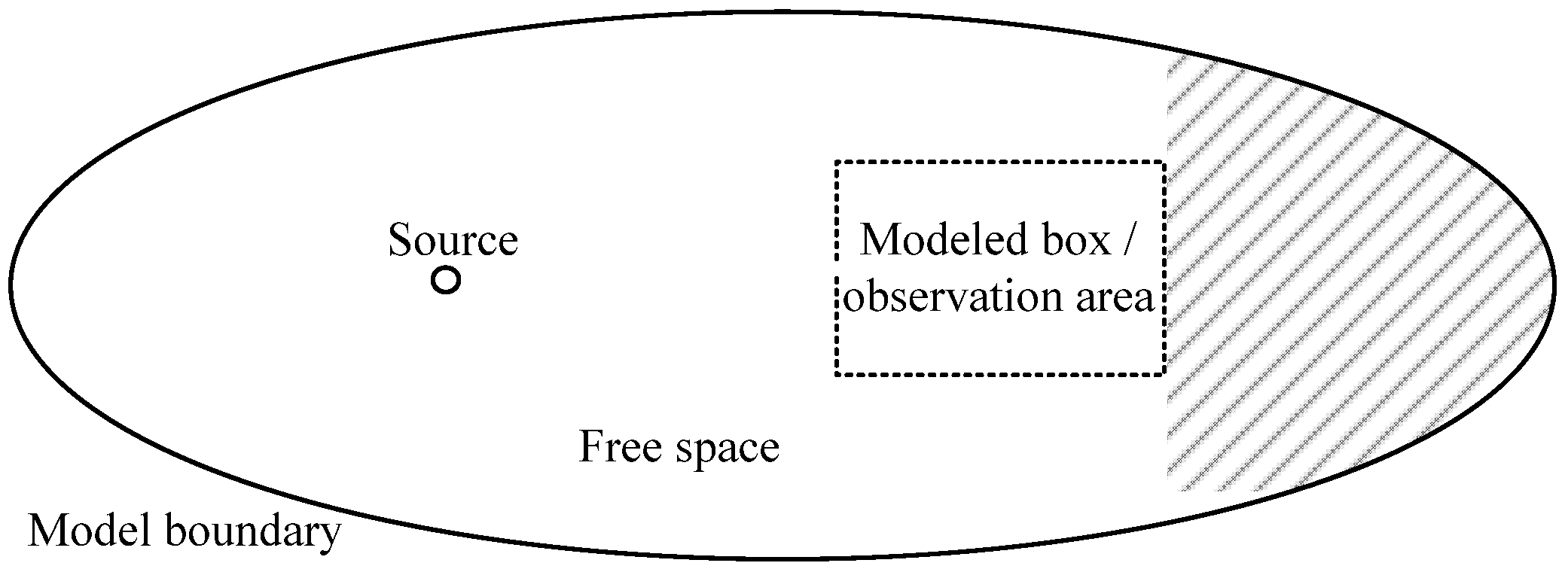
The most important numerical methods for SE simulation are the finite element method, finite difference time domain method, method of moments, and their modifications. The general geometries of the models are similar for all these methods, but the definitions—initial and boundary conditions, distribution of mesh—could be different. The model consists of a free space surrounding the excitation source and geometry of the shielding enclosure (see
Figure 1). Of course, from the definition of the SE, there is necessary to calculate two models—one with the enclosure and one without it (only with the observation area of the same dimensions as the internal dimension of the enclosure).
The setting of correct boundary conditions of the model is necessary for obtaining correct results. For example, the model boundary is usually modeled as a perfect magnetic () or electric () conductor, but a better choice is to use perfectly matched layer (PML), where the transition of the source signal is improved. The boundary of the box should be modeled as a perfect electric conductor (PEC), when the material of the box is made from a highly conducting material. The definition of the source depends on the method used, and for FEM it is possible to use a source of electric or magnetic field.
The SE simulations can be solved in two or three dimensions. For a 2D simulation, it is necessary to compute two models represented by two slices of the enclosure. Two sets of results from 2D simulations exhibit results comparable with a 3D simulation. The main difference is in the solution time, the 3D simulation requires much longer time. On the other side, 2D FEM models can be calculated by a solver with
hp-adaptivity of the mesh, which provides very accurate results [
8].
2. 3D Finite Element Method (FEM) Numerical Model
For finite element analysis in the frequency domain, the governing wave equation can be written as:
where μ
r represents the relative permeability, ε
r stands for the relative permittivity, σ is electric conductivity, ε
0 represents the vacuum permittivity, and
k0 is the wave number of free space defined by the equation:
The source is modeled as an electric point dipole, the vector of electric current dipole moment being .
The shielding box is approximated by a PEC, where:
For the analysis of fringing fields, a sphere of air was added around the model that is overlaid with a perfectly matched layer (PML). PML absorbs all radiated waves with small reflections by stretching the virtual domains into the complex plane using the following coordinate transform for the general space variable
t:
where Δ
w is the width of the PML region,
n represents the PML order, λ is the frequency, and
F denotes the scaling factor. The imaginary unit
i satisfies the equation
i2 = − 1.
3. Illustrative Example
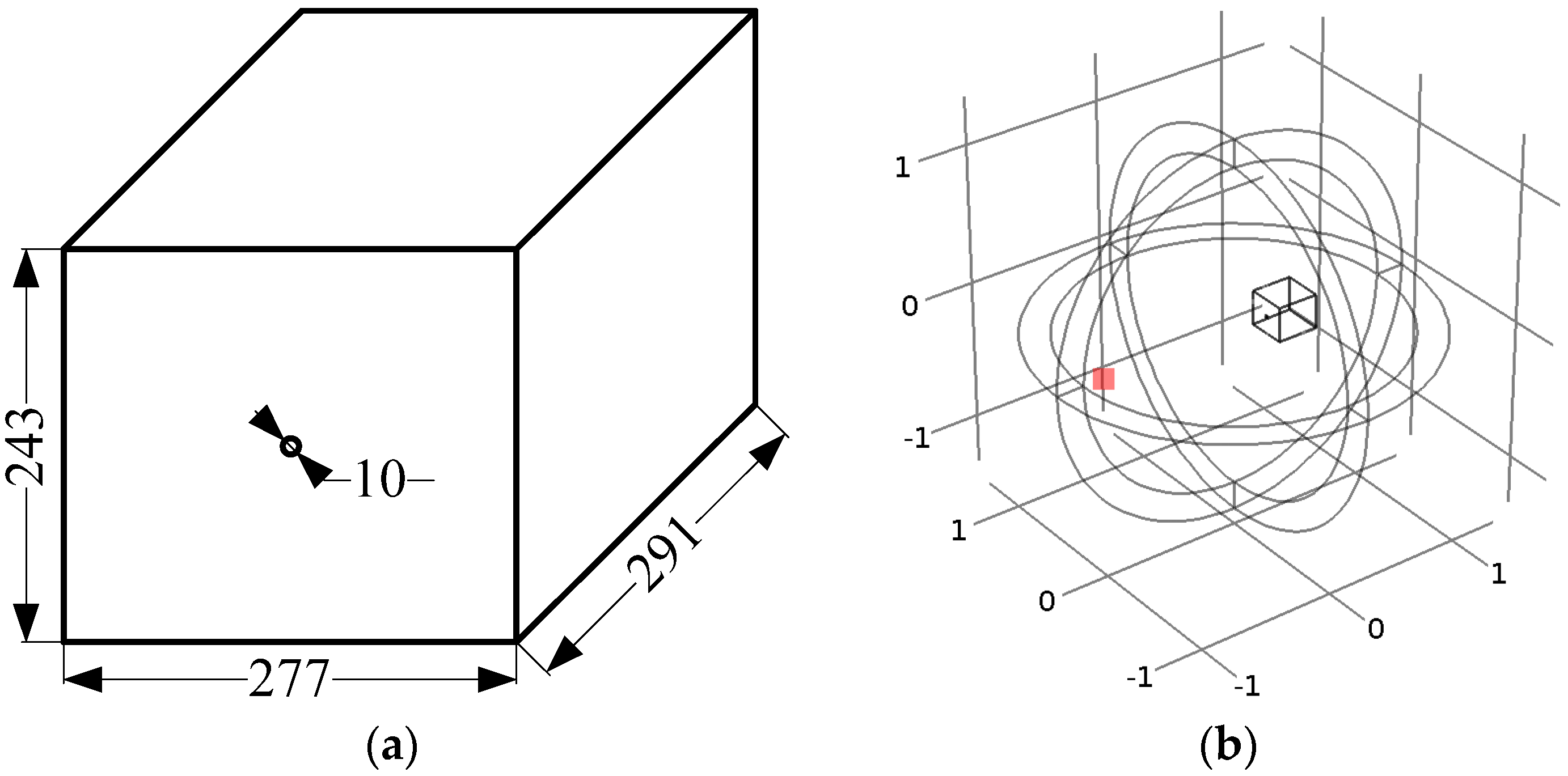
A rectangular prism shielding enclosure was used for this illustrative example of SE simulation. Its dimensions are 291 mm × 277 mm × 243 mm and the thickness of its wall is 1 mm. The circular aperture of 10 mm diameter is placed in the center of the area 277 mm × 243 mm (see
Figure 2a). The cavity dimensions are 289 mm × 275 mm × 241 mm.
Figure 2b represents a spherical area of the FEM model. There are visible four regions, the first of them representing the PMLs (on the model boundary) followed by a free space (surrounding enclosure). Inside the free space region there are placed the excitation source and shielding enclosure. The model represents the worst case; radiation from the source impacts the wall with the aperture. All parts were computed using Equations (8)–(11) by the software COMSOL Multiphysics.
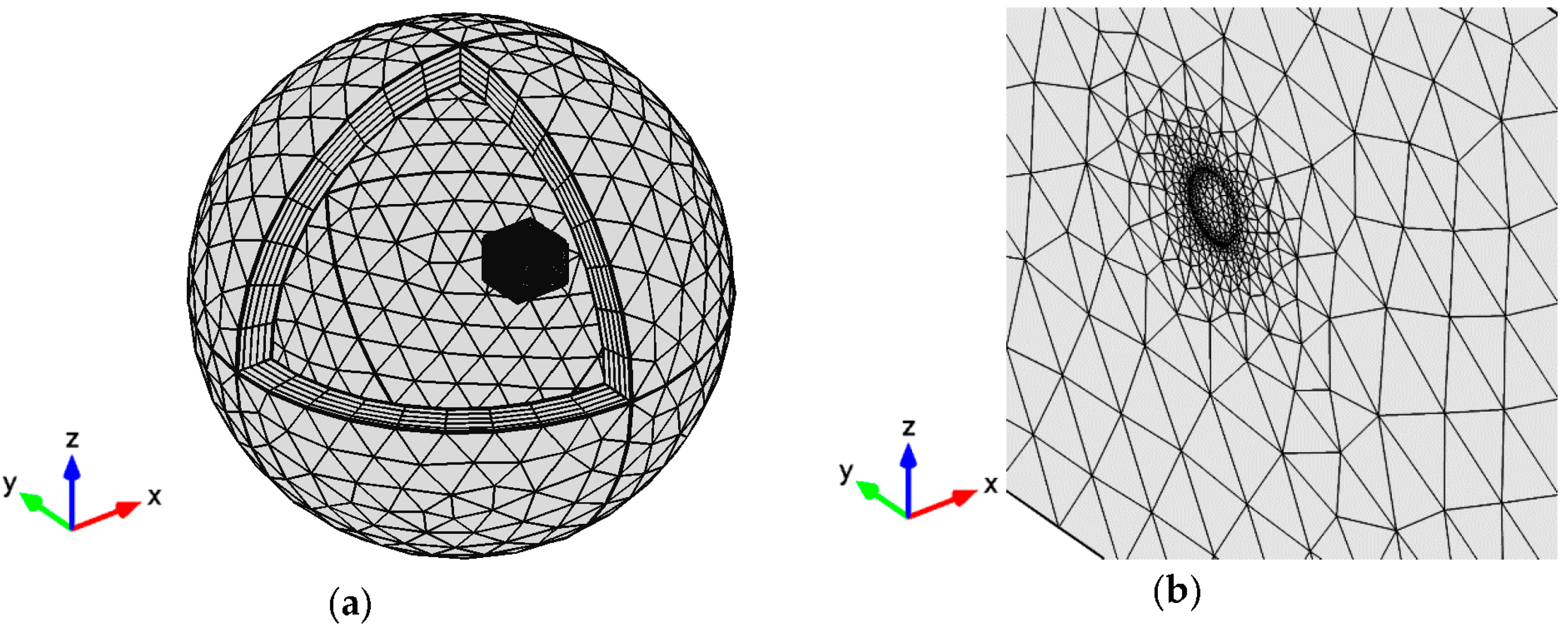
The FE mesh is shown in
Figure 3. The size of the mesh was chosen with respect to the accuracy of the model—its important parts (shielding enclosure, free space area) were meshed more densely, while for PMLs we used sparser mesh. Five layers were used for modeling PMLs.
The model was solved in the frequency domain. The simulation started at 500 MHz and ended at 2500 MHz. The frequency step—with respect to the computation time—was chosen 2.5 MHz. Overall, 800 simulation runs were carried out.
Important part of the simulation is verification of the result accuracy. Computing of the total electric energy inside the model is one possibility to check the solution accuracy:
where V represents the whole volume of the model and energy W
e is calculated from the expression:
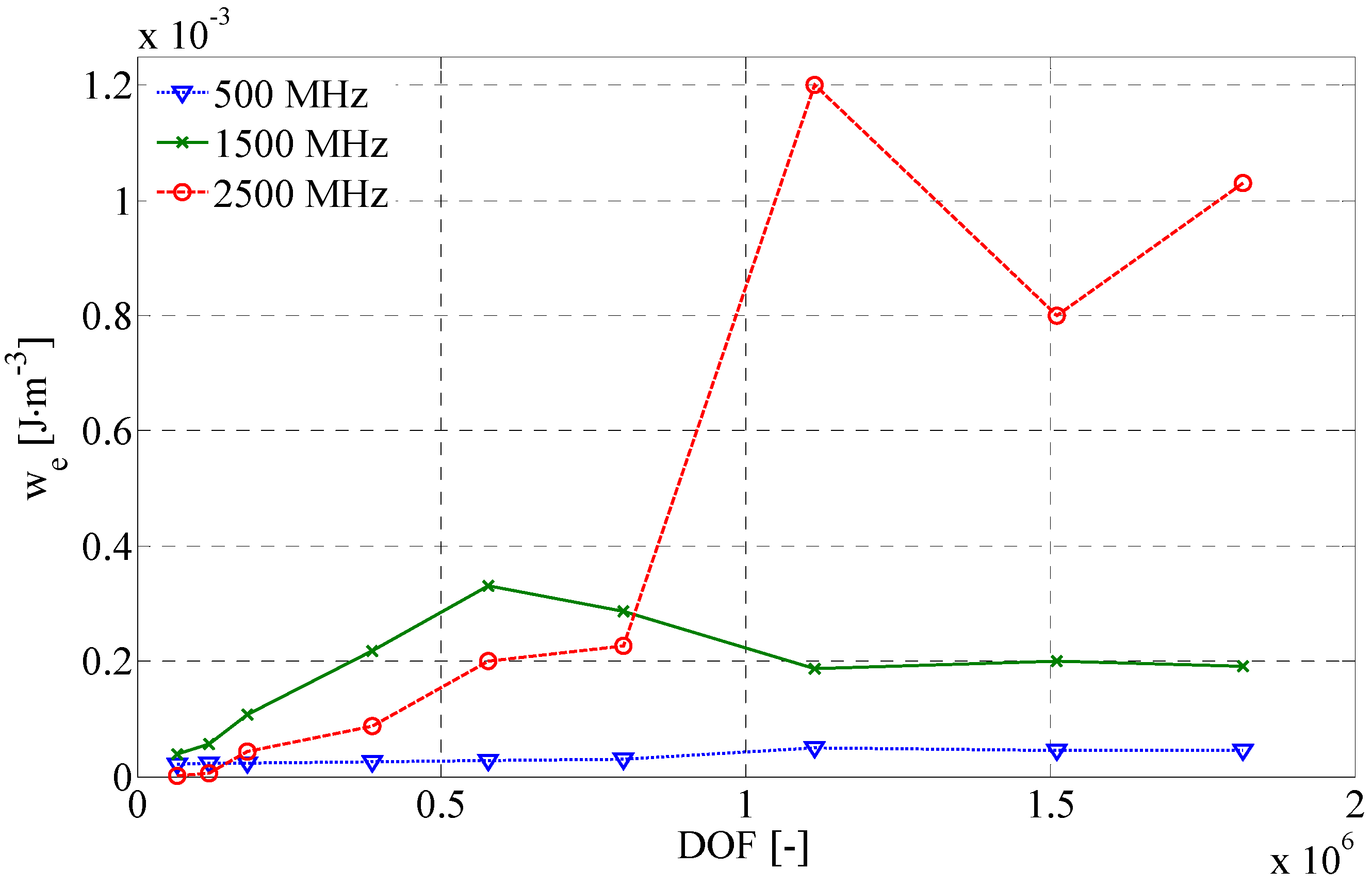
The accuracy of the solution is good if the total electric energy does not change with the number of the degrees of freedom (DOFs). For the same number of DOFs, the accuracy will be better for lower frequencies; much more DOF must be used for high frequencies.
Figure 4 shows the dependences of total electric energies on the number of DOFs of the model. There are three dependences corresponding to frequencies 500 MHz, 1500 MHz and 2500 MHz. The accuracy of the result at 500 MHz is obviously good. Different situation occurs with frequency 1500 MHz; the good accuracy of result begins at 1.15 million of DOFs. The worst situation is at frequency 2500 MHz—the total electric energy of the model is changing and the accuracy of the result cannot be guaranteed. A model with more DOF must be solved for high frequencies. The solution of such a model with a high number of DOF, however, requires longer calculation time and higher demands on hardware.
Examples of simulation results are shown in
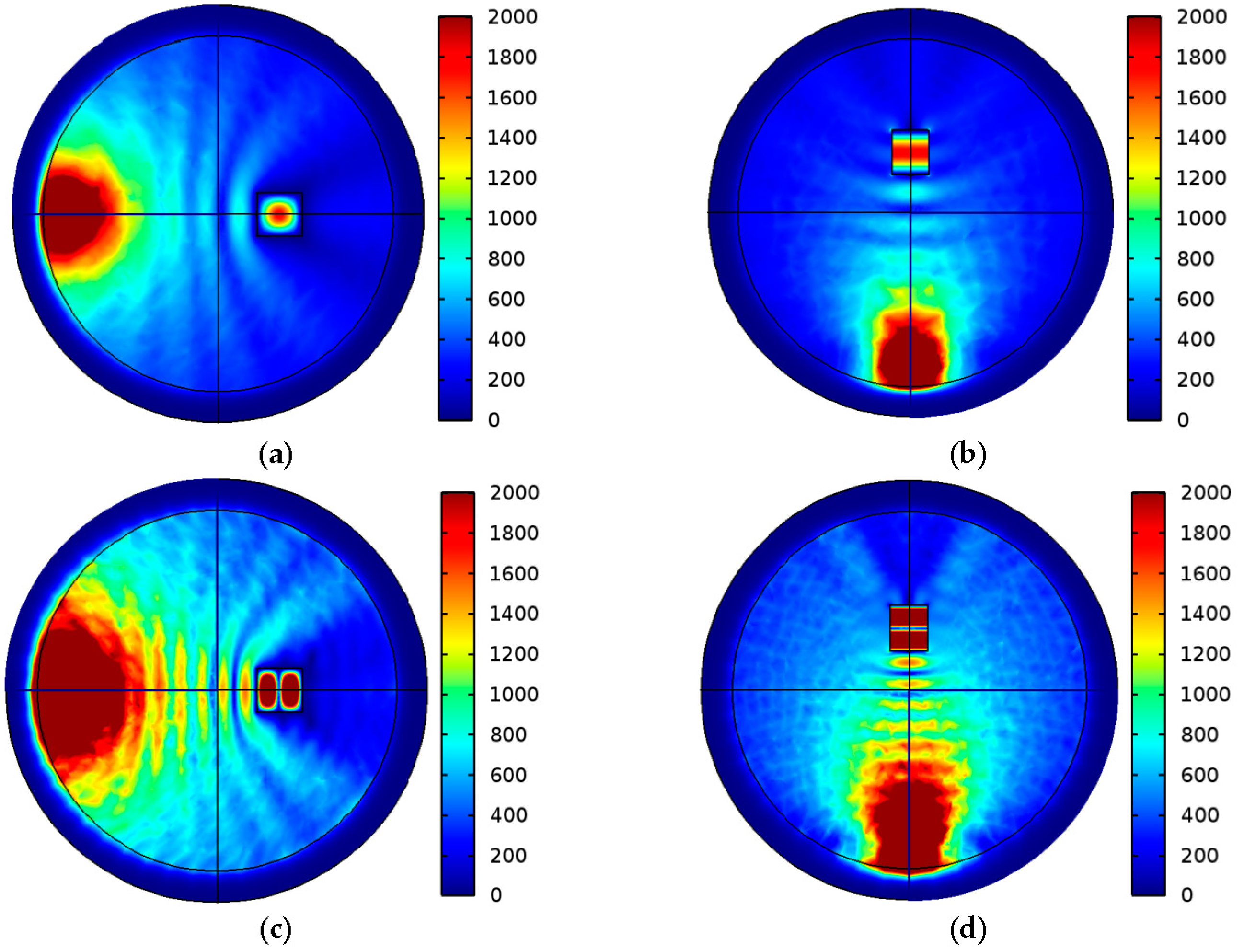
Figure 5 and
Figure 6. These figures represent distributions of electric fields in the model at frequencies 752.5 MHz and 1172.5 MHz. The frequency 752.5 MHz responds to the lowest resonance mode of the cavity (theoretically at frequency 752.94 MHz).
Figure 5 represents a sectional view of the model. There can be seen its slices in the
x-y plane and
z-
x plane, respectively.
There are visible minima and maxima of electric field inside the cavity; if the field is changing in any direction, it responds to resonance mode 1 (or higher) in the same direction. One change from minimum to maximum and again back to minimum (or inverse) represents one index of the resonance mode. No change of electric field responds to zero resonance mode indexes. The first resonance mode TE110 is at the frequency 752.5 MHz, (
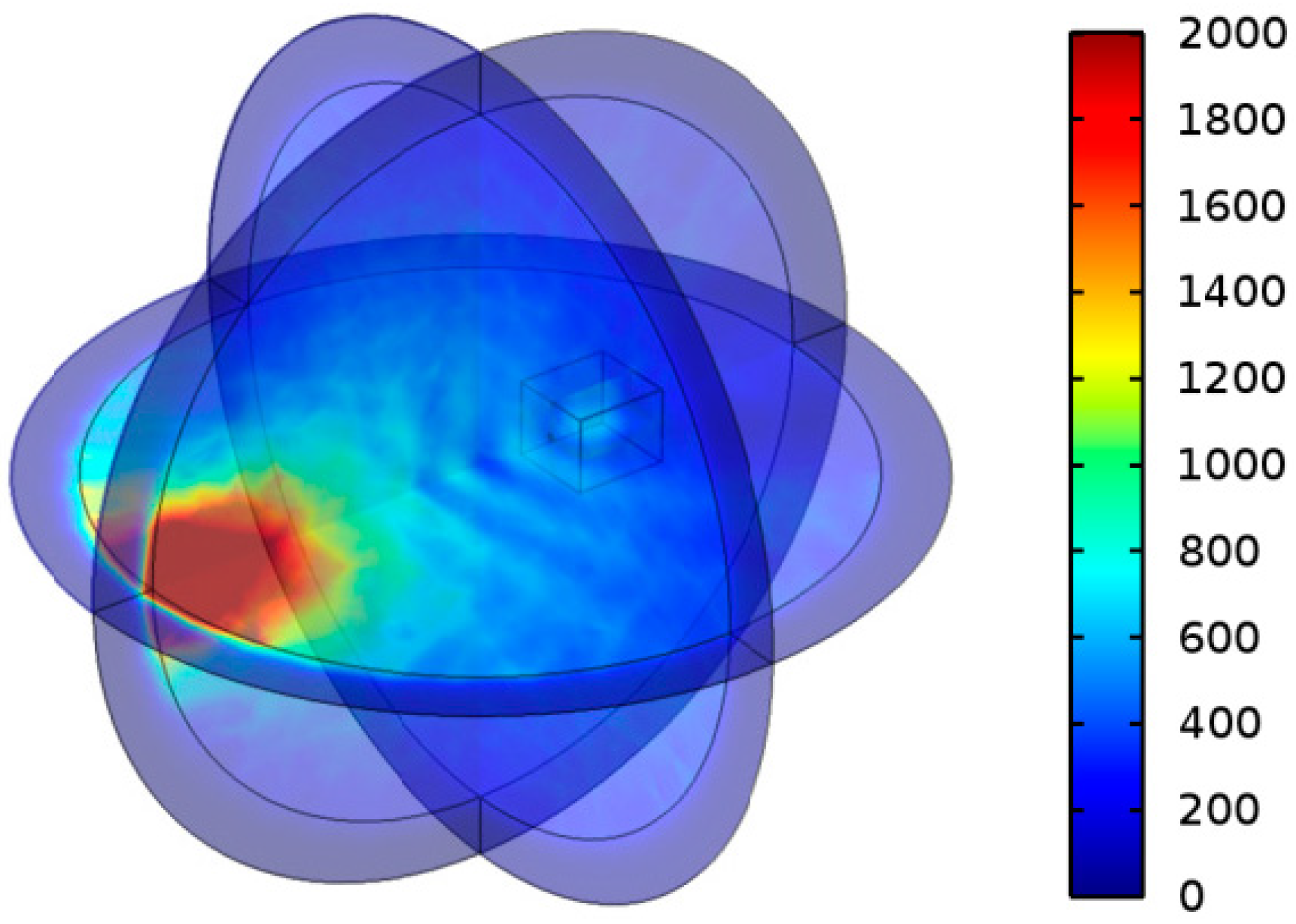
x-y-z axes, dimensions 289 mm × 275 mm × 241 mm). A 3D view of the same solution is shown in
Figure 6.
Figure 7 shows the dependence of simulated GSE on frequency and theoretical SE of circular aperture placed in ideally shielding plate that is calculated from Equation (6). There are visible influences of cavity resonances on SE—drops on the GSE trace, which represent decreases of GSE. Each drop responds to one TE resonance mode of the cavity. Of course, no drops of SE occur in the theoretical dependence.
4. Measurement Methods
The shielding effectiveness is defined by Equations (1), (2) and the measurement methods are based on the following principle; there is measured electric (or magnetic) field at a point of the space with and without the shielding enclosure [
14,
15]. One measurement method with measuring antenna is shown in
Figure 8.
There is no problem with shielding effectiveness measurement of large enclosures—there are standards for their measurement [
1,
16,
17]. However, SE measurement methods are not unified [
18]. On the other hand, shielding effectiveness measurement of small enclosures is quite problematic. The dimensions of the measurement antenna or electromagnetic field probe are not negligible—which depends on the wavelength—and this parameter is limiting factor for shielding effectiveness measurement of small enclosures, where it is necessary to place the measuring antenna inside the shielding enclosures. An antenna inside the enclosure represents another problem; the antenna represents filling of the cavity and it can influence the electromagnetic field inside it. The cavity filling influences space inside it and the resonance frequencies can be shifted.
The measurement should be performed in the far field region, where the characteristic impedance is conclusively defined; the theoretic distance is given by the expression:
where
r represents the transition between near and far fields and λ represents the wavelength.
In practice, the dimensions of the receiving antenna are often larger or comparable with the wavelength, and the distance between the near and far fields is defined by the Rayleigh criterion [
19]:
where
D represents the characteristic dimension of the receiving antenna.
5. Experimental Measurements
The experimental measurements were performed in the semi-anechoic chamber at the University of West Bohemia that is constructed for measurement at 3 m distance between the antenna and device under testing (DUT). This 3 m distance provides a uniform electromagnetic field in the frequency range from 26 MHz up to 18 GHz. The maximum value of electric field depends on the high-frequency power amplifier; for the 3 m distance we are able to produce 10 V/m in the frequency range from 80 MHz up to 3 GHz. Two types of HF power amplifiers are used: a FLH-200B (frequency range from 20 MHz to 1 GHz, maximum output power 200 W) and a FLG-30C (1–3 GHz, 30 W) and two types of antennas—BTA-M log periodic antenna (frequencies from 80 MHz to 2.5 GHz) and a BBHA 9120E horn antenna (500 MHz–6 GHz). For the measurement of electric field an ETS HI-6005 electric field probe was used.
The measurement method described in chapter Measurement Methods was used in this case, but the ETS HI-6005 electric field probe was replaced by a receiving antenna (see
Figure 8). The BTA-M log periodic antenna radiates the power from amplifiers. The first measurement was performed without the shielding enclosure; the electric field strength was measured with the E-field probe. The second measurement was performed with the shielding enclosure; the E-field probe was inserted inside the box. The shielding effectiveness was calculated from measured values using Equation (1).
The frequency range of experimental measurement for the enclosure dimensions (
Figure 2) is from 500 MHz to 2.5 GHz. The lowest frequency was set bellow the first cavity resonance of the enclosure. From the dimension of the cavity and Equation (5), the lowest cavity resonance frequency (and the first transversal electric mode TE110) is 752.94 MHz.
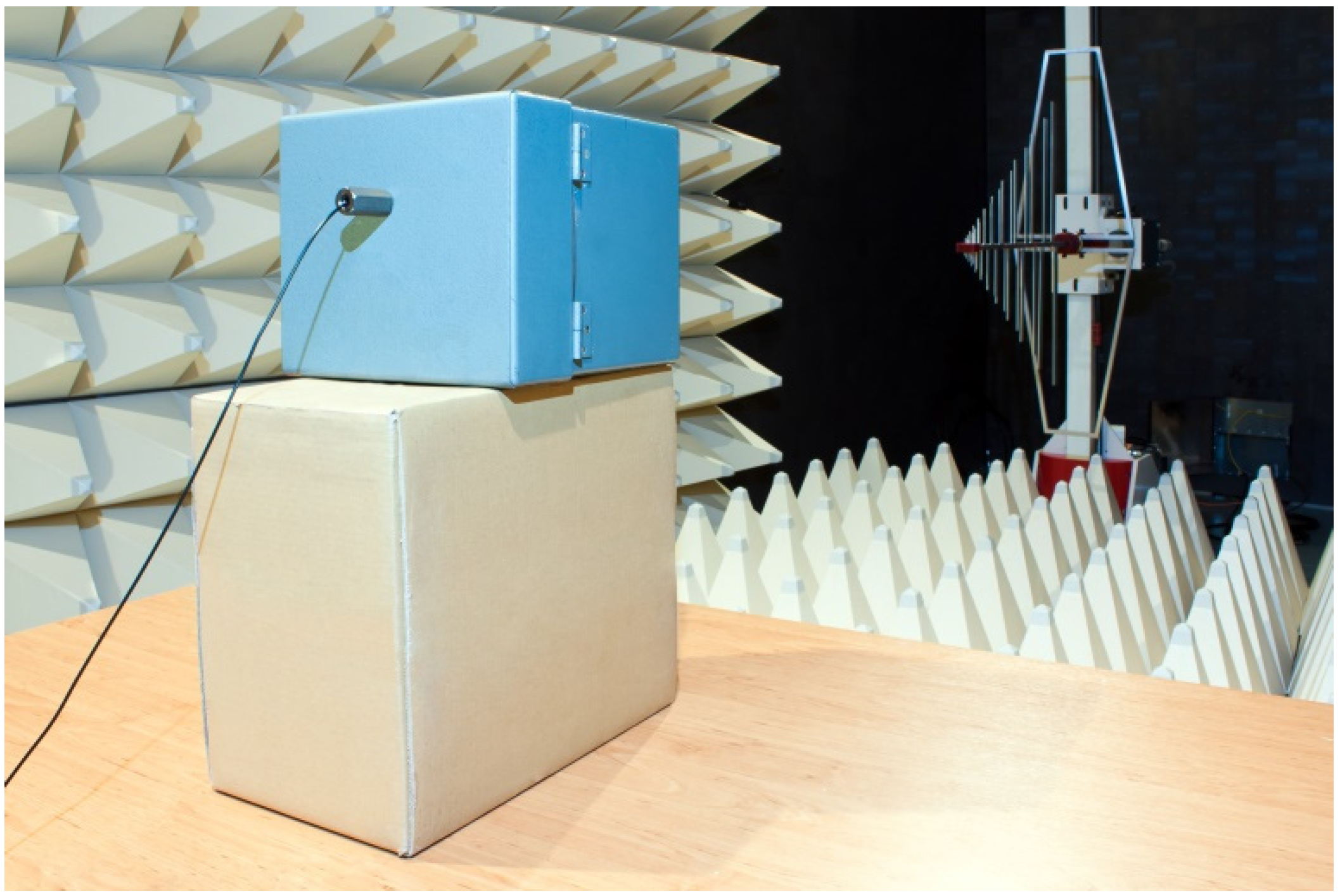
Figure 9 shows the experimental measurement in the semi-anechoic chamber. The shielding enclosure and optical cable from the electric field probe are visible in foreground (the paper box below the enclosure is the stand); the transmitting antenna and absorbers are visible in background. The optical cable was pulled through the cable gland representing a waveguide and the SE is not influenced by the next aperture in the shielding enclosure (the critical frequency of the waveguide is approximately 8.79 GHz).
6. Results Comparison
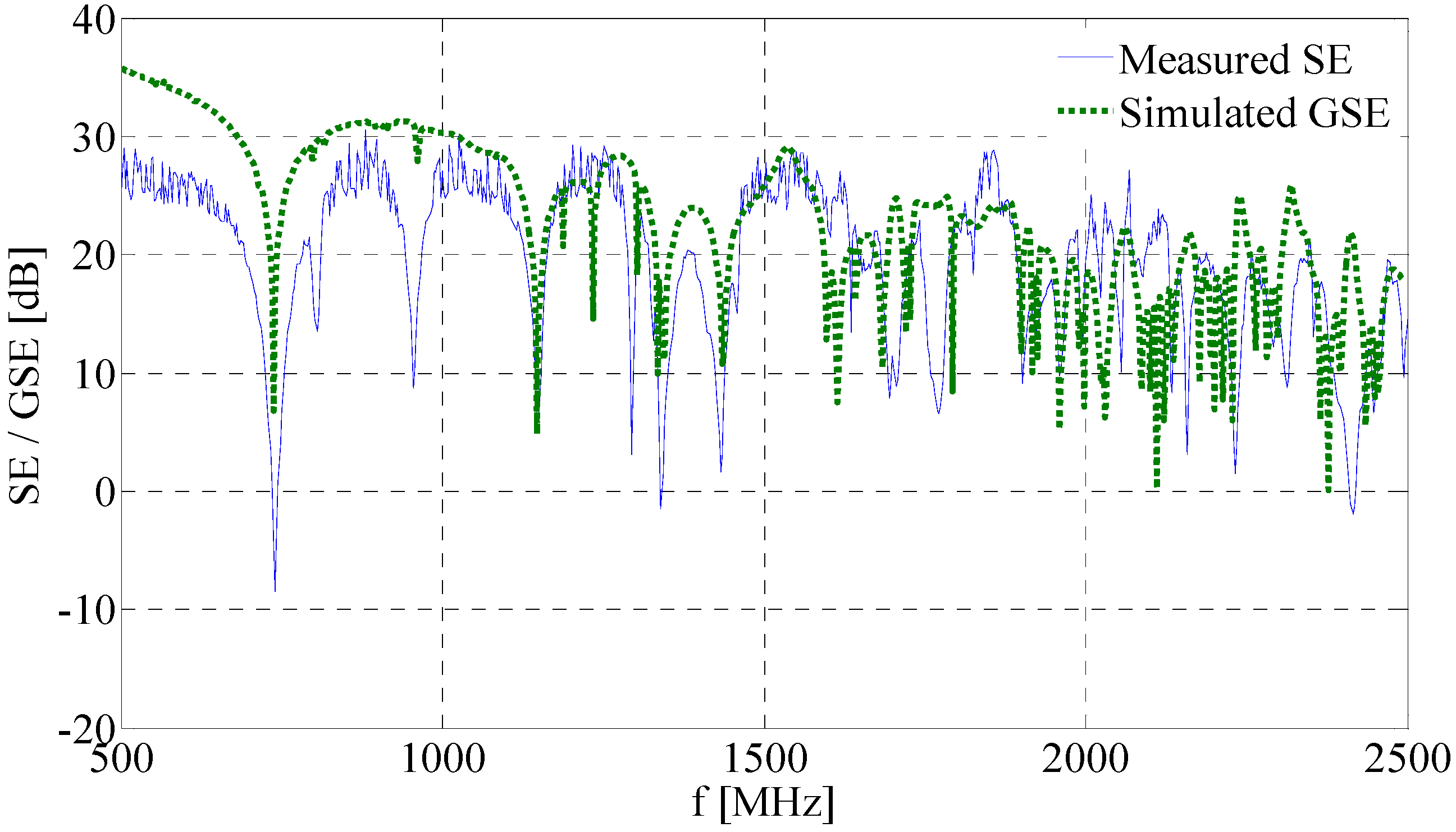
The simulated GSE dependence on frequency of the 3D model compared with the SE experimental measurement is shown in
Figure 10. There is visible a good agreement of the resonance frequencies. These frequencies are possible to be calculated using Equation (5). Small differences between the calculated and measured (or simulated) frequencies are caused by the 2.5 MHz steps of measurement (or simulation).
The values of GSE are almost better than the measured values; it could be caused by using of the PEC boundary condition for the shielding enclosure.
The simulation results for frequencies higher 2 GHz are tentative, because the convergence of the model is not guaranteed (see
Figure 4). The mean values are 23.39 dB for GSE and 23.59 dB for SE (the mean error being 0.2 dB).
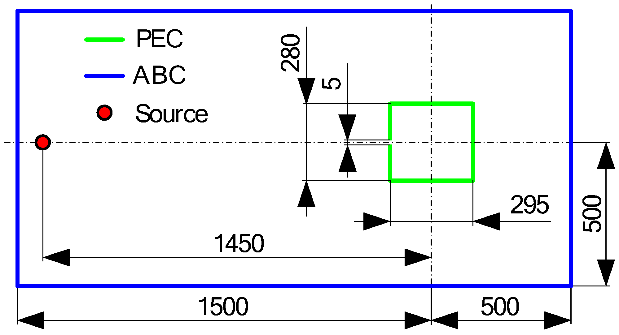
The 2D model definitions are shown in
Figure 11. The source representing an electric current dipole with current
I0 = 1 A is placed on the left. Absorbing boundary condition (ABC) was applied along the model boundary, which represents a free space surrounding model. The shielding box is approximated by a PEC.
The comparison between the 2D and 3D simulations of the GSE dependence on frequency is shown in
Figure 12. The results from one 2D simulation are shown here, while other results of 2D simulations including results of the
hp-adaptivity models were described in [
8]. These results correspond with enclosure dimension 289 mm × 275 mm (it represents a slice of the 3D model in the
z-axis). There are only TExx0 modes for 2D simulations; higher modes in the
z-axis cannot be calculated. Another simulation (model which represents a
y-axis slice of the 3D model) must be solved for determining of all TE modes.
7. Conclusions
This paper describes the problems with determining the shielding effectiveness of perforated shielding enclosures. General shielding effectiveness theory was defined for a perfect environment and conditions, but this theory does not correspond with real cases—these are influenced by dimensions of antennas (vs. spot observation points in general SE theory). For this reason a new definition called global shielding effectiveness (GSE) was established. Even when there exist standards for measurement of the SE, these are applicable only in certain cases, where large enclosures are examined, but these measurement methods are not applicable for very small enclosures having the smallest linear dimension smaller than 2.0 m.
Numerical methods can be helpful for determining of SE. There are lots of numerical methods (FEM, FDTD, MoM, etc.) which are used for SE calculations. The paper presents the FEM model of the perforated shielding enclosure, various definitions and geometries are discussed. The 3D model is supplemented with the complete set of results, while the 2D model only with a part of results. The disadvantage of 3D models is large hardware requirement and long solution time. 2D models are not time consuming. Also hp-adaptivity of FE mesh can be used for 2D models, in this case it is guaranteed the correctness of results (the convergence of the model from the mathematical viewpoint).
The verification of the numerical results using the total electric energy inside the model is an important part of the paper. The dependence of the total electric energy on DOF shows the solution accuracy; the model with more DOF must be solved for high frequencies (with the same accuracy as for low frequencies with a lower number of DOF). This solution, however, requires longer computational time and more powerful hardware. The simulation results were verified by measurements. Our measurement method uses a small electric field probe instead of receiving antenna, the dimensions of the probe correspond to a cube with 70 mm edge. The experimental measurement was performed in a semi-anechoic chamber and it was based on general SE theory (however, the dimensions of the electric field probe are not negligible—it is not a dot observation point). The probe dimensions allow SE measurement of a small shielding enclosure with dimensions of less than 2.0 m.
The miniaturization of electronic devices provides a space for SE numerical calculations—there are no possibilities for SE measurement (or very limited). The importance of numerical calculations for shielding effectiveness in the future, therefore, will grow. The future research will be focused on SE simulation and measurement of the complex perforated shielding enclosures, including ventilation structures or cable glands.
Acknowledgments
This research has been supported by the Ministry of Education, Youth and Sports of the Czech Republic under the RICE—New Technologies and Concepts for Smart Industrial Systems, project No. LO1607 and by the project SGS-2015-002.
Author Contributions
Both authors contributed equally to this work. Both authors performed the measurement and designed the simulations, discussed the results and commented on the manuscript at all stages.
Conflicts of Interest
The authors declare no conflict of interest. The founding sponsors had no role in the design of the study; in the collection, analyses, or interpretation of data; in the writing of the manuscript, and in the decision to publish the results.
Abbreviations
The following abbreviations are used in this manuscript:
| FEM | Finite element method |
| GSE | Global shielding effectiveness |
| SE | Shielding effectiveness |
| FDTD | Finite difference time domain method |
| MoM | Method of moments |
| ABC | Absorbing boundary condition |
| PEC | Perfect electric conductor |
| DOF | Degrees of freedom |
References
- Institute of Electrical and Electronics Engineers (IEEE). IEEE standard method for measuring the effectiveness of electromagnetic shielding enclosures. In IEEE Std 299–2006 (Revision of IEEE Std 299–1997); IEEE: New York, NY, USA, 2007; pp. 1–52. [Google Scholar]
- Robinson, M.P.; Benson, T.M.; Christopoulos, C.; Dawson, J.F.; Ganley, M.D.; Marvin, A.C.; Porter, S.J.; Thomas, D.W.P. Analytical formulation for the shielding effectiveness of enclosures with apertures. IEEE Trans. Electromagn. Compat. 1998, 40, 240–248. [Google Scholar] [CrossRef]
- Liu, E.; Du, P.-A.; Nie, B. An extended analytical formulation for fast prediction of shielding effectiveness of an enclosure at different observation points with an off-axis aperture. IEEE Trans. Electromagn. Compat. 2013, 56, 589–598. [Google Scholar] [CrossRef]
- Araneo, R.; Lovat, G.; Celozzi, S. Compact electromagnetic absorbers for frequencies below 1 GHz. Prog. Electromagn. Res. 2013, 143, 67–86. [Google Scholar] [CrossRef]
- Olyslager, F.; Laermans, E.; De Zutter, D.; Criel, S.; De Smedt, R.; Lietaert, N.; De Clercq, A. Numerical and experimental study of the shielding effectiveness of a metallic enclosure. IEEE Trans. Electromagn. Compat. 1999, 41, 202–213. [Google Scholar] [CrossRef]
- Lozano-Guerrero, A.J.; Diaz-Morcillo, A.; Balbastre-Tejedor, J.V. Resonance suppression in enclosures with a metallic-lossy dielectric layer by means of genetic algorithms. In Proceedings of the IEEE International Symposium on Electromagnetic Compatibility (EMC 2007), Honolulu, HI, USA, 9–13 July 2007; pp. 1–5.
- Li, M.; Nuebel, J.; Drewniak, J.L.; DuBroff, R.E.; Hubing, T.H.; Van Doren, T.P. EMI from cavity modes of shielding enclosures-FDTD modeling and measurements. IEEE Trans. Electromagn. Compat. 2000, 42, 29–38. [Google Scholar]
- Kubik, Z.; Skala, J. Influence of the cavity resonance on shielding effectiveness of perforated shielding boxes. In Proceedings of the 8th International Conference on Compatibility and Power Electronics (CPE), Ljubljana, Slovenia, 5–7 June 2013; pp. 260–263.
- Kubík, Z.; Karban, P.; Pánek, D.; Skála, J. On the shielding effectiveness calculation. Computing 2013, 95, 111–121. [Google Scholar]
- Hromadka, M.; Kubik, Z. Suggestion for changes in shielding effectiveness measuring standard. In Proceedings of the 4th International Youth Conference on Energy (IYCE), Siófok, Hungary, 6–8 June 2013; pp. 1–4.
- Celozzi, S. New figures of merit for the characterization of the performance of shielding enclosures. IEEE Trans. Electromagn. Compat. 2004, 46. [Google Scholar] [CrossRef]
- Tesche, F.M.; Ianoz, M.V.; Karlsson, T. EMC Analysys Methods and Computational Models; John Wiley & Sons Inc.: New York, NY, USA, 1992; ISBN 0-471-15573-X. [Google Scholar]
- Chatterton, P.A.; Houlden, M.A. EMC Electromagnetic Theory to Practical Design; John Wiley & Sons Ltd.: Chichester, UK, 1992; ISBN 0-471-92878-X. [Google Scholar]
- Holloway, C.L.; Ladburry, J.; Coder, J.; Koepke, G.; Hill, D.A. Measuring shielding effectiveness of small enclosures/cavities with a reverberation chamber. In Proceedings of the IEEE International Symposium on Electromagnetic Compatibility, Honolulu, HI, USA, 9–13 July 2007; pp. 1–5.
- Greco, S.; Sarto, M.S. Hybrid mode-stirring technique for shielding effectiveness measurement of enclosures using reverberation chambers. In Proceedings of the IEEE International Symposium on Electromagnetic Compatibility, Honolulu, HI, USA, 9–13 July 2007; pp. 1–6.
- Institute of Electrical and Electronics Engineers (IEEE). IEEE recommended practice for measurement of shielding effectiveness of high-performance shielding enclosures. In IEEE Std 299–1969; IEEE: New York, NY, USA, 1969. [Google Scholar]
- United States Military Standard MIL-STD-285. Method of Attenuation Measurements for Enclosures, Electromagnetic Shielding, for Electronic Test Purposes; U.S. Government Printing Office: Washington, DC, USA, 1956.
- Butler, J. Shielding effectiveness—why don’t we have a consensus industry standard? In Proceedings of the Professional Program Proceedings Electronics Industries Forum of New England, 1997, Boston, MA, USA, 6–8 May 1997; pp. 29–35.
- IEEE. IEEE standard definitions of terms for radio wave propagation. In IEEE Std 211–1997; IEEE: New York, NY, USA, 1998. [Google Scholar]
Figure 1.
General description of SE model.
Figure 1.
General description of SE model.
Figure 2.
(a) Dimensions of shielding enclosure in millimeter; (b) area of the FEM model. The excitation source is placed at the red point, the enclosure is placed on the opposite side of the model. Here the dimensions are in m.
Figure 2.
(a) Dimensions of shielding enclosure in millimeter; (b) area of the FEM model. The excitation source is placed at the red point, the enclosure is placed on the opposite side of the model. Here the dimensions are in m.
Figure 3.
Distribution of the FE mesh. (a) FE mesh in the whole model. There are visible five layers of the PMLs, the black box inside the model represents a very fine FE mesh of the shielding enclosure; (b) detail of the FE mesh around the circular aperture of the enclosure.
Figure 3.
Distribution of the FE mesh. (a) FE mesh in the whole model. There are visible five layers of the PMLs, the black box inside the model represents a very fine FE mesh of the shielding enclosure; (b) detail of the FE mesh around the circular aperture of the enclosure.
Figure 4.
Total energy dependence on degree of freedom in the model with shielding enclosure. Example of the model convergence for frequencies 500 MHz, 1.5 GHz and 2.5 GHz.
Figure 4.
Total energy dependence on degree of freedom in the model with shielding enclosure. Example of the model convergence for frequencies 500 MHz, 1.5 GHz and 2.5 GHz.
Figure 5.
Distribution of the electric field E [V/m] in the model: (a) Frequency 752.5 MHz, x-y plane; (b) frequency 752.5 MHz, z-x plane; (c) frequency 1172.5 MHz, x-y plane; and (d) frequency 1172.5 MHz, z-x plane.
Figure 5.
Distribution of the electric field E [V/m] in the model: (a) Frequency 752.5 MHz, x-y plane; (b) frequency 752.5 MHz, z-x plane; (c) frequency 1172.5 MHz, x-y plane; and (d) frequency 1172.5 MHz, z-x plane.
Figure 6.
Distribution of electric field E [V/m] in the 3D model, frequency 752.5 MHz.
Figure 6.
Distribution of electric field E [V/m] in the 3D model, frequency 752.5 MHz.
Figure 7.
Simulation result of global shielding effectiveness (GSE) from 3D FEM model compared with theoretical calculation of SE for a circular aperture. Drops in the simulated results are caused by cavity resonances.
Figure 7.
Simulation result of global shielding effectiveness (GSE) from 3D FEM model compared with theoretical calculation of SE for a circular aperture. Drops in the simulated results are caused by cavity resonances.
Figure 8.
Experimental shielding effectiveness measurement in an anechoic chamber. This method uses transmitting and receiving antennas, while the control and evaluation of the measured data is provided by a personal computer.
Figure 8.
Experimental shielding effectiveness measurement in an anechoic chamber. This method uses transmitting and receiving antennas, while the control and evaluation of the measured data is provided by a personal computer.
Figure 9.
Experimental measurement in the anechoic chamber. The shielding enclosure is placed on the paper stand (set 1.5 m above ground in the axis of the transmitting antenna) in the foreground of the picture, the transmitting log-per antenna is placed in the background of the picture.
Figure 9.
Experimental measurement in the anechoic chamber. The shielding enclosure is placed on the paper stand (set 1.5 m above ground in the axis of the transmitting antenna) in the foreground of the picture, the transmitting log-per antenna is placed in the background of the picture.
Figure 10.
Comparison of results between measured SE and simulated GSE of 3D model.
Figure 10.
Comparison of results between measured SE and simulated GSE of 3D model.
Figure 11.
Area of the 2D FEM model, including dimension in millimeters and setting of the boundary conditions.
Figure 11.
Area of the 2D FEM model, including dimension in millimeters and setting of the boundary conditions.
Figure 12.
Comparison of results between global shielding effectiveness of the 2D and 3D FEM model simulations.
Figure 12.
Comparison of results between global shielding effectiveness of the 2D and 3D FEM model simulations.
© 2016 by the authors; licensee MDPI, Basel, Switzerland. This article is an open access article distributed under the terms and conditions of the Creative Commons by Attribution (CC-BY) license (http://creativecommons.org/licenses/by/4.0/).


