1. Introduction
The concept of energy saving includes a variety of techniques aimed at reducing the energy consumption needed for the different human activities. Nowadays, a great deal of attention has been given to efficient energy use in the heating and cooling sector, and building envelopes play a crucial role in the reduction of the energy consumption and the related costs. In fact, building heating and cooling are responsible for about 40% of the final energy consumption in the European Union (EU) and, as a consequence, for a considerable amount of total CO
2 emissions [
1]. The attention to the issue of energy efficiency in buildings is demonstrated by international and national directives [
2,
3,
4,
5], which describe the procedure for energy certification of buildings, and require member states to ensure that new and existing buildings meet minimum energy performance requirements, monitoring the actual energy demand or the estimated energy necessary to meet the various needs related to standard building uses, such as heating and cooling.
In this perspective, the methodology used to calculate the heat losses through the building envelope plays a crucial role, as well as the correct determination of the constitutive properties of the materials used. In many cases, one-dimensional and two-dimensional models do not correctly reproduce the heat transfer and vapor diffusion through the components of the building enclosure, but it is necessary to employ three-dimensional numerical models capable of solving the partial differential equations through the actual building envelope, characterized by the presence of geometric and structural non-uniformities, defined as thermal bridges.
These, characterized by a multi-dimensional heat flow and a consequent lowering of internal surface temperatures, are also those structures in which condensation and mold growth phenomena occur, due to incorrect design of the building envelope from the hygrothermal point of view. In this regard, the verification of hygrothermal performance [
6] has the purpose of determining the possible presence of water condensed in a part of the examined structure, and then proceed to its correct design in order to avoid such critical phenomenon. Despite the requirements concerning the insulation of buildings, specified by national and international regulations, thermal bridges are a weak spot in constructions, since are often not dealt with properly. For example, the presence of inhomogeneities (
i.e., metal stud) inside construction materials is often not taken into account, despite the consequent results could be very different, as shown in this work. These aspects lead to underestimate the heat losses during the design stage, therefore providing lower insulation levels for the building envelope, with consequent higher actual energy consumption, if compared to the estimates [
7]. It should be pointed out that the use of different calculation methods of thermal bridges, provided in standards [
8,
9], can lead to different energy performance classes of a building and to percentage gaps on the energy requirements in the heating season, calculated to be more than 20% [
10].
In this scenario, the use of numerical tools, required by the standards for the characterization of thermal bridges [
9], should be extended to the verification of hygrothermal performance of these structures, given the complexity of solving the governing equations analytically. In these analyses, the thermal and hygrometric properties employed for each material of the building envelope assume a crucial role. These properties are available for most building components [
11,
12,
13], or must be certified by the manufacturer and are commonly used in design calculations. However, problems may arise for inhomogeneous materials, such as concrete, heavily used in the existing building envelopes. In fact, the presence of steel stud strongly influences the thermal conductivity and the hygrometric properties of the inhomogeneous concrete structure. The adoption of the value of thermal conductivity of simple concrete may cause significant errors in the calculation of the actual heat losses. Furthermore, neglecting the presence of the metal stud, some areas of possible water condensation may be ignored, thus preventing the subsequent corrective action.
Therefore, the authors’ aim in this work is to show the importance of taking into account the presence of inhomogeneities inside construction materials. This approach, referred to as “microscopic”, requires to reproduce the inhomogeneities (i.e., metal stud), with their physical properties, inside the geometry under investigation.
The present paper is structured as follows: the next section provides a review of the available literature on numerical modelling of thermal bridges, and introduces the novelties of the present paper, then the mathematical model employed is described in section three. The fourth section shows the influence of the inhomogeneities inside building structures, while the fifth section reports the verification of the obtained results for a benchmark problem. The sixth section presents the main results obtained for the three-dimensional thermal bridge taken into account and for a room envelope, while some conclusions are drawn in the last section.
2. Review of the Available Literature
The importance of quantifying the heat loss through thermal bridges is well recognized in engineering practice, and technical standards provide a way to approximate the behavior of thermal bridges under steady design conditions. However, in order to take into account actual transient conditions, a number of works have studied thermal behavior of linear thermal bridges, to analyze their contribution to the total energy performance of buildings. The phenomenon depends on several factors, such as external and internal conditions, level of insulation, geometry of the thermal bridge and materials used, structure and use of building, and the results of calculations, unlike reality, often depend on the model used to calculate its effects on building energy demand [
14]. Therefore, estimates of the actual weight of thermal bridges on the energy demand of buildings can vary from 5%, in the case of retrofitting the exterior of the building envelope, to 39% in well insulated single family houses without proper thermal bridge treatment [
14].
Due to the complexity of three-dimensional (3D) unsteady simulations, most studies use one-dimensional (1D) and two-dimensional (2D) approaches or steady-state regime. A review of methods for dynamic modelling of thermal bridges in building envelopes is reported in [
15]. Moreover, most commercial software for the dynamic simulation of thermal performance of buildings assume 1D heat transfer neglecting 2D dynamic heat conduction through the thermal bridges of building enclosures [
16].
An earlier work of Kosny and Christian [
17] showed that thermal resistance of a concrete wall reinforced with metal stud may decrease of about 48% because of the steel-concrete thermal bridge effects. The authors employed a finite difference algorithm for the simulation of transient heat transfer in building walls and wall corners. Moreover, Kosny and Kossecka [
18] demonstrated, by using a 3D finite difference algorithm, that the thermal resistance of walls, calculated neglecting the thermal bridge effects and adopting the one-dimensional approach, might be overestimated of more than 44%. Gao
et al. [
16] used a reduction technique to simulate three-dimensional heat transfer. The work focused on the study of the dynamic behavior of thermal bridges in a simplified form by using a commercial simulation software. The study showed that thermal bridges are responsible for an increase in the overall heat loss of the building taken into account from 9% to 19%. Mao and Johannesson [
19] developed a code based on a frequency response approximation method to calculate temperatures and heat fluxes in thermal bridges, by using the finite element discretization technique. Déqué
et al. [
20] integrated a 2D dynamic modeling of thermal bridges into a commercial software, showing that this approach can lead to a difference of 7% in heat losses evaluated with the use of tabulated values. An interesting 3D numerical study on the influence of outdoor environmental conditions on building energy performance has been carried out by He
et al. [
21] by using a proprietary algorithm, but neglecting the presence of thermal bridges in the building envelope. Recently, Tadeu
et al. [
1] proposed a 2D dynamic model, based on the boundary element method in the frequency domain, to characterize wall corners and estimate their influence on the thermal performance of building components. Theodosiou
et al. [
22] carried out 3D heat transfer simulations of cladding systems for building facades, showing that neglecting the point thermal bridge effect in these kind of systems can lead to a significant underestimation (from 5% to 20%) of actual heat flows.
Some combined experimental and numerical works are also available in the literature. Nussbaumer
et al. [
23] analyzed both experimentally and numerically a concrete wall with external insulation of polystyrene boards, containing vacuum insulation panels, demonstrating the thermal improvement obtainable with this type of insulation. Wakili
et al. [
24] reproduced numerically, with a 3D commercial code, steady-state temperature field in a balcony board with integrated glass fiber reinforced plastic elements. Numerical results, combined with experimental data, proved that a reduction of heat losses are obtainable by using glass fiber reinforced elements instead of conventional steel rods. Zalewski
et al. [
25] employed a 3D commercial code for steady state analysis of thermal efficiency of complex building walls, focusing on the estimation of heat losses from thermal bridges. The authors also carried out an experimental analysis by using infrared thermography and heat flow meters for quantitative characterization of the losses through the envelope. A recent work by Lorenzati
et al. [
26] investigated the influence of thermal bridges on the overall energy performance of Vacuum Insulation Panels (VIP). They showed that the use of equivalent values for thermal conductivity of VIP could lead to significant errors in the estimation of thermal bridges’ effects.
The above literature review proves the technical-scientific interest for the calculation of heat losses through thermal bridges, given the significant influence that these components of a building have on the global heat losses of buildings. To the authors’ knowledge, some aspects on this subject are not dealt with in depth in the available literature. In particular, the above literature review shows that a microscopic approach that takes into account the presence of inhomogeneities inside construction materials has not been employed coupled with 3D numerical simulations of thermal bridges under dynamic conditions. Furthermore, the verification of hygrothermal performance in presence of inhomogeneous materials, which is a crucial aspect for building structures, has not been extended to 3D thermal bridges. On the basis of these considerations, in this work the authors, experienced in the field of numerical simulation of complex thermo-fluid-dynamics problems and energy saving systems [
27,
28,
29,
30], investigate the influence of inhomogeneities inside construction materials simulating transient heat conduction and vapor diffusion in 3D thermal bridges.
3. Mathematical Model
The mathematical model employed in the present work for the simulation of heat and mass transfer through a three-dimensional thermal bridge consists in the unsteady conservation equations for mass and energy in a homogeneous permeable medium. The governing equations have been solved by using the software Comsol Multiphysics. To employ the present microscopic approach, the governing equations are therefore written for each isotropic homogeneous material that is found in a typical building envelope:
Heat transfer by conduction Therefore, in order to take into account the presence of metal stud in the thermal bridge, Equation (1) is also solved in the domain occupied by the metal.
The set of partial differential Equations (1) and (2) are solved with the following boundary and initial conditions for energy and mass:
where
and
are the initial temperature and partial pressure of vapor, respectively,
and
are the convective heat transfer coefficients of the interior and exterior environment, respectively,
and
are the interior and exterior environment temperatures, respectively.
and
are the temperatures of the interior and exterior surfaces, respectively,
and
are the partial pressures of vapor in the interior and exterior environment. The mathematical model described above is solved by using the well known Finite Element Method [
31,
32].
The procedure for the verification of the hygrometric performance (Glaser’s method), based on the technical standard [
6], is here applied to thermal bridges. In order to avoid interstitial and superficial water condensation, the following condition must be satisfied in each point of the structure:
where
is the saturation pressure of water at temperature
T.
The relation between temperature and saturation pressure of water is given in [
6] as:
in which the temperature must be expressed in degrees Celsius (°C).
In common practice, the conditions characterized by a vapor partial pressure,
, larger than saturation pressure of water at a prescribed temperature,
, are not physical, because saturation pressure is the maximum vapor pressure compatible with the prescribed temperature value,
T. Therefore, inside the computational domain, wherever
, condensation occurs. The Glaser’s method applied to one-dimensional problems, such as those assumed in most building walls, allows to calculate the amount of water condensed in the wall as the difference between diffusive vapor flux entering and leaving the different layers of the wall [
33,
34]. This same type of analysis can be extended to three-dimensional problems, where condensation occurs in a volume delimited by surfaces (defined as
A and
B in the followings) on which the condition
is verified, while inside the volume the condition
occurs. Based on these considerations, the present numerical procedure is developed in order to estimate the rate of condensing water,
, in a three-dimensional structure when condition Equation (4) is not verified, from the difference between the calculation of vapor flux and vapor flux at saturation conditions, as follows:
where
is the diffusive vapor flux entering the condensation volume through surface
A, while
is the diffusive vapor flux calculated at saturation conditions leaving the condensation volume through surface
B:
where surfaces
A and
B cannot be defined a-priori, since they depend on the temperature distribution in the considered geometry.
4. Influence of Inhomogeneities inside Building Structures
Materials employed in building applications are commonly considered to be homogeneous and isotropic, and their thermal properties are often dependent on temperature and density. However, when inhomogeneous and anisotropic media are taken into account, the physical properties are different because of the inhomogeneities present inside the material.
In this section, the authors take into account two typical constructive elements: a concrete pillar with metal stud and a brick-concrete slab, in order to analyze the influence of the inhomogeneities on the heat flux transferred by these structures. The first case is presented in
Figure 1, which shows the three-dimensional profile of a concrete pillar
with and without the metal stud, together with section and stud details. Two different stirrup spacing are taken into account, 0.2 m and 0.1 m, in order to show the dependence of the heat flux on the construction characteristics. The materials considered are: (i) concrete of natural aggregates with closed structure and with a thermal conductivity
; (ii) steel, used as metal stud, with a thermal conductivity
[
11,
12,
13]. In order to calculate the heat flux transferred by different pillar configurations, it is necessary to reproduce the problem numerically under steady-state and specified boundary conditions. The boundary conditions employed are:
where the convective heat transfer coefficients are taken from technical standard [
35], while the interior temperature is provided in [
36,
37]. The value of the exterior temperature considered is the design value referred to the city of Napoli in Italy, given in the technical standard [
38].
The simulation of steady-state heat transfer allows to calculate, in the post-processing stage, the heat flux transferred from the exterior environment to the interior one.
Table 1 reports the heat flux calculated for the three concrete pillar configurations. The presence of the metal stud in the concrete pillar leads to an increase of 6.8% of the heat flux if the metal stud with stirrup spacing of 0.2 m is considered, and 8.9% if the metal stud with stirrup spacing of 0.1 m is considered. From the analysis of the data presented in
Table 1, it is evident that the presence of a steel stud in the concrete pillar has an influence on the heat flux transferred from the structure. This calculation should be carried out each time the amount of steel in the pillar changes.
The second case, presented in
Figure 2, shows the three-dimensional profile of a concrete slab
and of a brick-concrete slab, together with the details of the brick-concrete section. The materials considered are (i) concrete of natural aggregates with closed structure with a thermal conductivity
; (ii) steel rods with a thermal conductivity
; (iii) bricks with a thermal conductivity
[
11,
12,
13].
The boundary conditions employed are represented by Equations (8). The values of heat flux calculated by means of numerical simulation are reported in
Table 1. It should be pointed out that the presence of the bricks strongly influences the heat flux transferred from the interior to exterior surface of the slab. In fact, the value of this parameter decreases of 30% with respect to the case of pure concrete (
Table 1).
These results highlight the difference in terms of heat flux due to the presence of inhomogeneities inside construction materials, by using a microscopic approach. However, in order to correctly characterize a building structure in terms of both heat transfer and vapor diffusion, unsteady simulations should be carried out. In addition, the presence of inhomogeneities must be necessarily taken into account, by using the present microscopic approach, as shown for the two configurations of thermal bridges and for the room envelope presented in
Section 6. With this approach, the actual building structure is numerically reproduced, and the physical properties of the materials reported in the technical standards [
11,
12,
13] are considered. Therefore, the use of non-physical parameters, such as equivalent values of physical properties, is avoided. Before showing these results, the required verification of the numerical model is presented in the next section.
5. Verification of the Numerical Model
The results obtained by using the present numerical model are verified against the reference data available in technical standard [
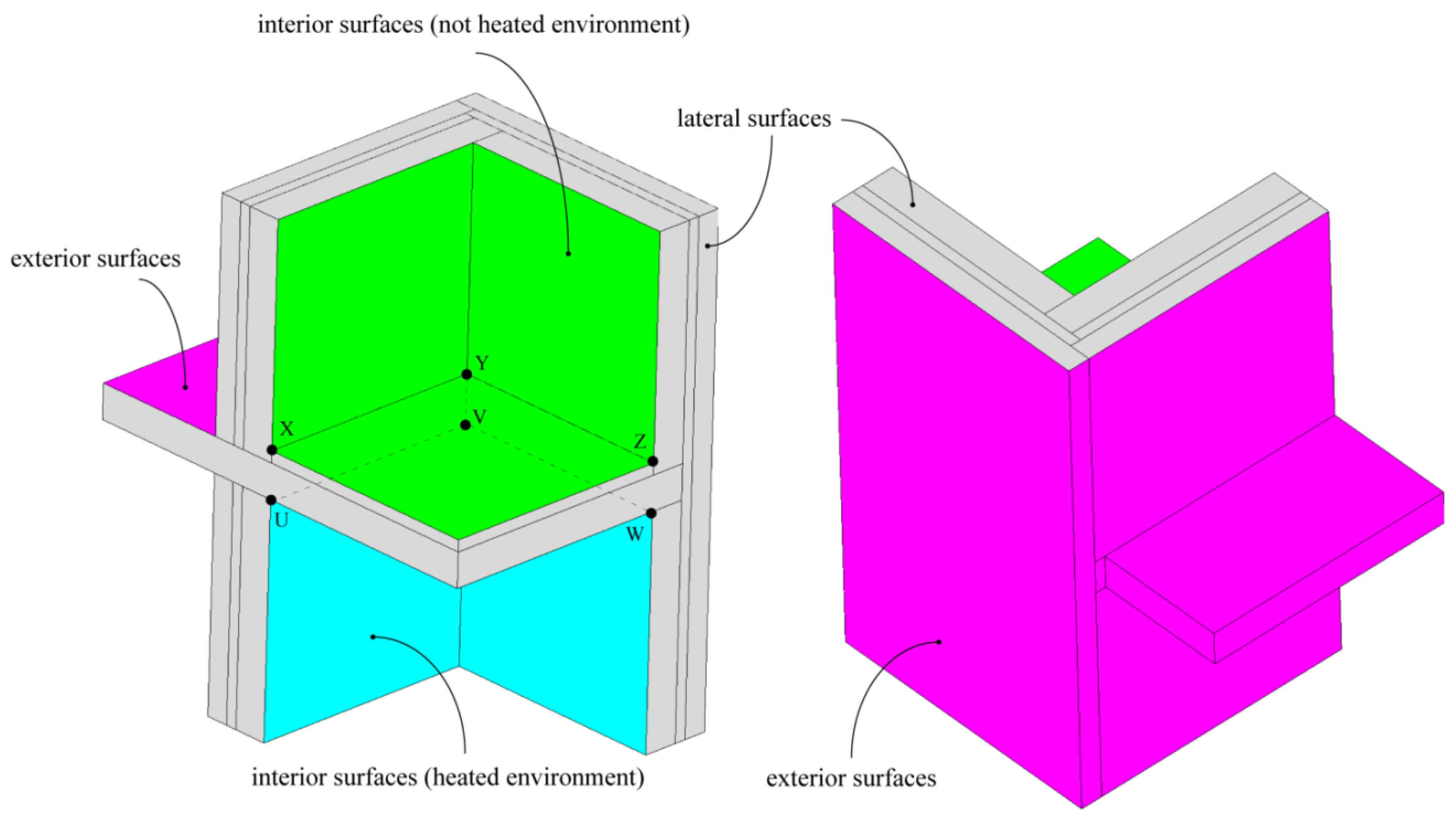
9] for steady-state heat transfer through a three-dimensional thermal bridge. The geometry of the benchmark problem considered and the description of the surfaces with different boundary conditions are depicted in
Figure 3. The computational domain consists of a three-dimensional structure that separates three environments kept at different temperatures. More details necessary for defining the geometry are available in reference [
9]. The boundary conditions employed in the simulations, with reference to the surfaces highlighted in
Figure 3, are:
The computational grid employed is made of 72010 nodes and 383715 tetrahedral elements. The mesh has been chosen after grid sensitivity analysis, in order to ensure that all the calculated values are mesh independent. Grid independency is considered to be achieved when the maximum difference between the quantities of interest calculated with a mesh and those obtained with the next finer grid is smaller than 1%.
The verification of the results against reference data [
9] is presented in
Table 2. The points and surfaces considered for temperature calculation are reported in
Figure 3. In order to consider the numerical model verified, the technical standard [
9] requires a difference between the calculated temperatures and reference data to be less or equal to 0.1 K, and a difference on the obtained heat flow rate and reference values less equal than 2%. From the analysis of
Table 2, it is evident that the present results are in perfect agreement with the data provided in [
9], and the above requirements are verified.
6. Numerical Results
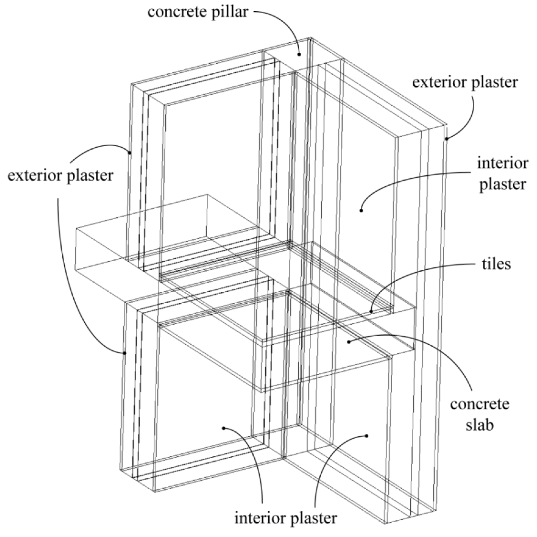
In the present work, the authors have simulated both steady-state and unsteady conduction heat transfer and diffusion of vapor in a three dimensional (3D) thermal bridge. The geometry considered for the numerical analysis is similar to the one proposed in the technical standard [
9], opportunely modified to reproduce a structure adopted in actual constructions. In particular, a pillar
is inserted at the corner, and the presence of interior and exterior plasters and of tiles is considered.
Furthermore, in order to show the importance of taking into account the presence of internal inhomogeneities of the materials employed in constructions to correctly estimate heat losses and condensation, two different cases are considered: the pillar and the slab are made of concrete of natural aggregates with closed structure (case 1); a steel stud in the pillar and a brick-concrete slab are considered (case 2). The 3D structures for the two cases of modified thermal bridge are reported in
Figure 4 and
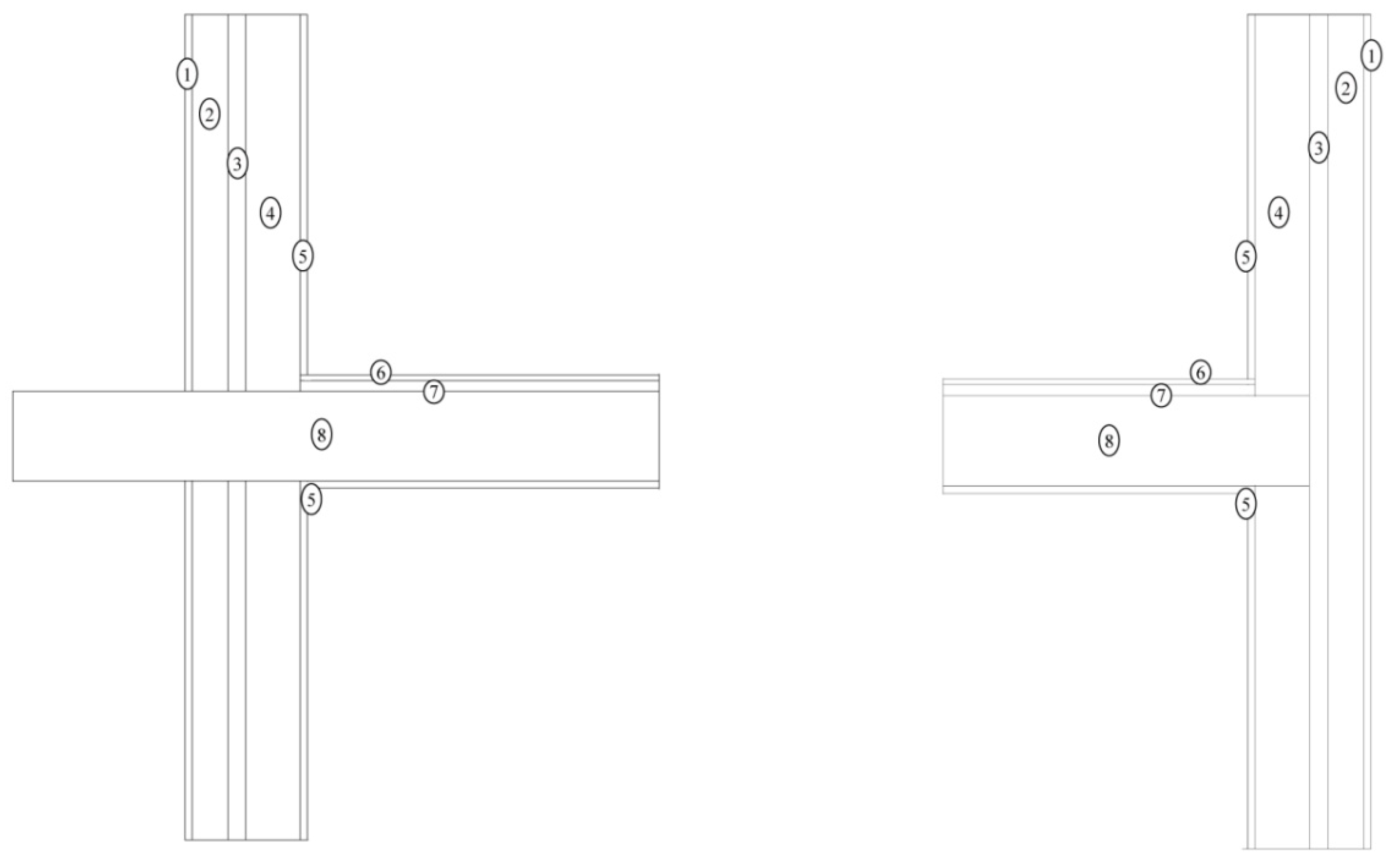
Figure 5, respectively, while the wall and slab sections are reported in
Figure 6. The physical properties of the materials employed in the modified thermal bridge, taken from the technical standards [
11,
12,
13], together with their geometrical characteristics, are reported in
Table 3. The geometry of thermal bridge corresponding to case 2 is the same as that studied by one of the authors in a recent paper [
39], where the aim was to analyze experimentally and numerically the effects of innovative materials employed in building structures.
In addition to the 3D thermal bridge, the authors analyze numerically a room of an apartment located at the top floor of a building.
6.1. Thermal Bridge under Steady-State Conditions
The boundary conditions employed for the solution of steady-state heat transfer are represented by Equations (9), but with different values of
: 7.7
, 7.7
and 25
, respectively, as required in technical standard [
35]. The boundary conditions employed for the solution of steady-state vapor diffusion, referred to the same surfaces considered for heat transfer and highlighted in
Figure 3, are:
From the obtained numerical results, reported in
Table 4 in terms of the heat flux transferred by the interior and exterior surfaces of the thermal bridge, it is possible to appreciate significant differences between case 1 and case 2. The difference on the heat flux calculated for case 1 and case 2, due to the presence of inhomogeneities in case 2, reaches the 16%. Obviously, these results depend on the geometry and on the construction characteristics of the structures considered in the simulations, and the percentage gap can increase for larger amount of steel or smaller bricks.
Table 4 also reports the results obtained when the properties corresponding to reinforced concrete are used (case 1.b), taken from the technical standard [
13]. In particular, a thermal conductivity of
has been used in the simulations, instead of the value of
reported in
Table 3. When the property value corresponding to reinforced concrete is considered, the differences with case 2 are larger with respect to the previous case 1.
Moreover, from the analysis of
Figure 7, which shows the temperature contours for the two thermal bridge configurations considered, it is clear that the temperature distribution in the thermal bridge is different in case 1 and case 2. In fact, the inhomogeneities in the structure cause a temperature decrease, particularly evident on the lower floor (blue color in
Figure 3), as shown in
Figure 7, on the right.
Table 4 reports the rate of water condensing in the thermal bridge, which increases by about 12% when inhomogeneities are taken into account.
6.2. Thermal Bridge under Unsteady Conditions
The two configurations of the thermal bridge, whose 3D profiles are reported in
Figure 4 and
Figure 5, are also studied under unsteady conditions. In particular, the time-dependent exterior temperature and partial pressure of vapor are considered in the simulations. The vapor partial pressure is calculated on the basis of time-dependent relative humidity,
, and time-dependent saturation pressure of water,
, as:
. Therefore, the boundary conditions employed for the solution of transient heat transfer are the same of the previous section for the interior and lateral surfaces, while on the exterior surfaces are:
The boundary conditions employed for the solution of transient vapor diffusion are represented by Equations (10) for the interior and lateral surfaces, while on the exterior surfaces are:
As initial conditions for both dynamic heat transfer and vapor diffusion, the solution obtained from the steady state simulations has been employed. The values of time-dependent exterior temperature,
, and time-dependent relative humidity,
, are calculated for the city of Aosta in Italy on the basis of the technical standard [
40], that reports the methodology to be employed for the definition of the reference year to be used to reproduce the climatic conditions. One week hourly simulation has been carried out for the coldest week of the reference year, with temperature values ranging between 9.1 °C and −6.3 °C (
Figure 8).
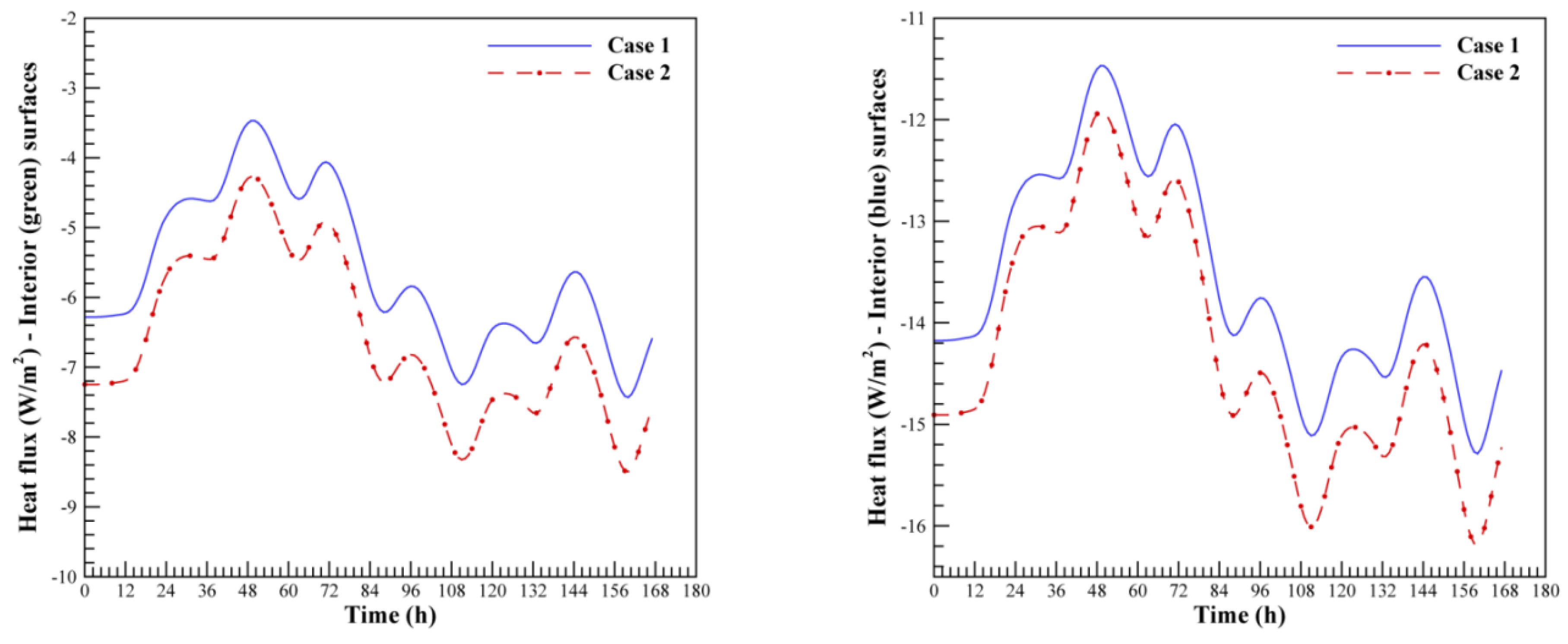
Figure 9 reports the heat flux transferred from the interior surfaces of the two configurations of thermal bridge over the coldest week of the year for the city of Aosta. It is evident that the presence of inhomogeneities causes a different thermal behavior of the structure. In particular, the difference of heat flux between the two cases is almost constant during the week considered in the simulations, since the presence of insulation between the bricks dampens the oscillations of the exterior temperature.
Figure 10 and
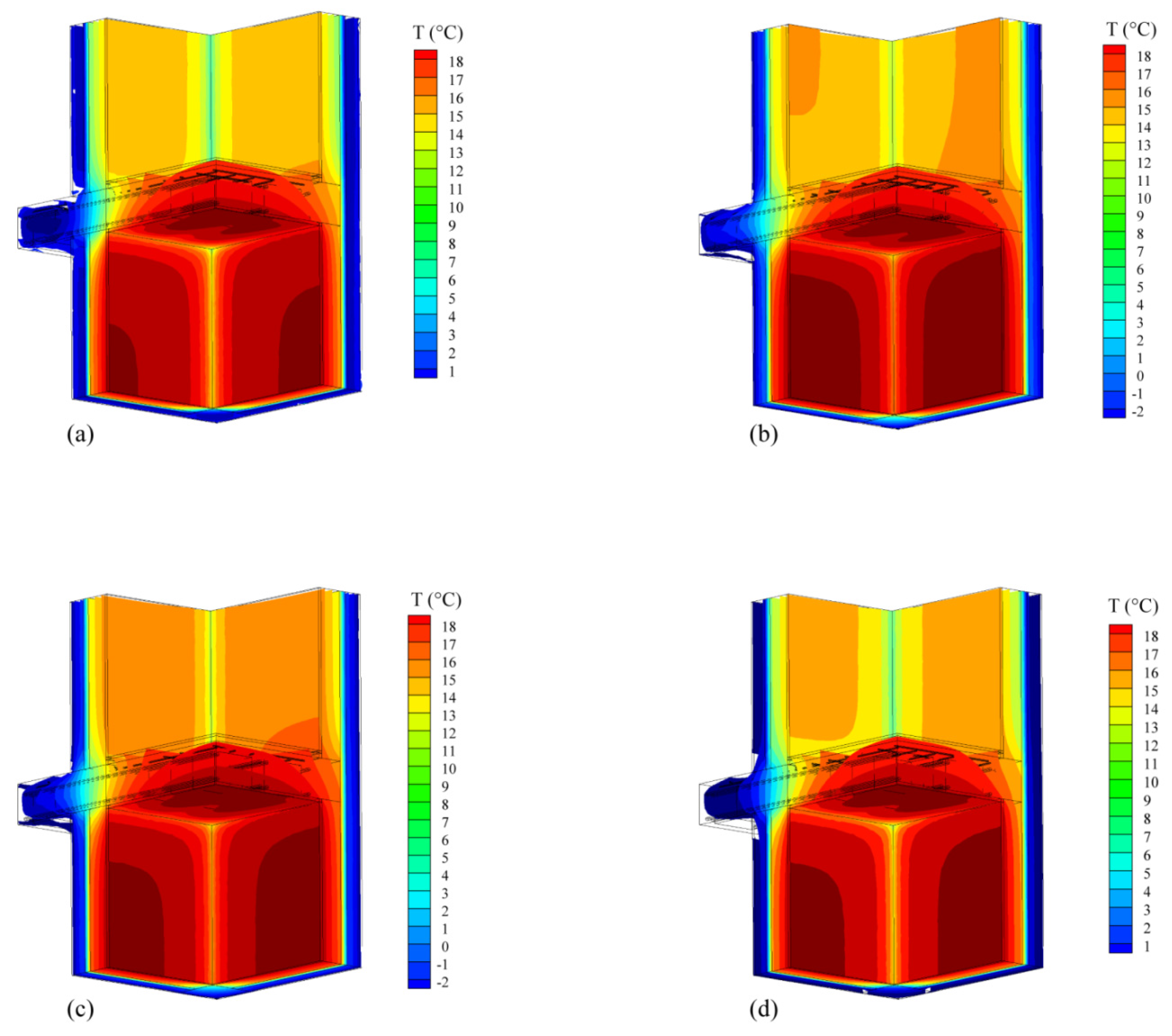
Figure 11 show the temperature contours obtained for case 1 and case 2, respectively, at four different times (12, 48, 96 and 168 h). From the analysis of these figures, it can be noticed that the temperature distribution in the two configurations of thermal bridge is significantly different at all the time instants presented, due to the inhomogeneities of case 2.
Figure 12 shows the variation of temperature at point V of
Figure 3 for the two cases of thermal bridge considered. This trend confirms the difference in the thermal behavior of the structure, introduced by the metal stud and the brick-concrete slab.
Figure 12 also shows the rate of condensed water,
, during the considered week. Only positive values of
are reported in
Figure 12, meaning that condensation occurs in the structure. From the analysis of the figure, it is clear that the inhomogeneities present in the thermal bridge result in different amounts of condensed water, confirming the differences found in the steady-state simulations.
6.3. Building Envelope under Unsteady Conditions
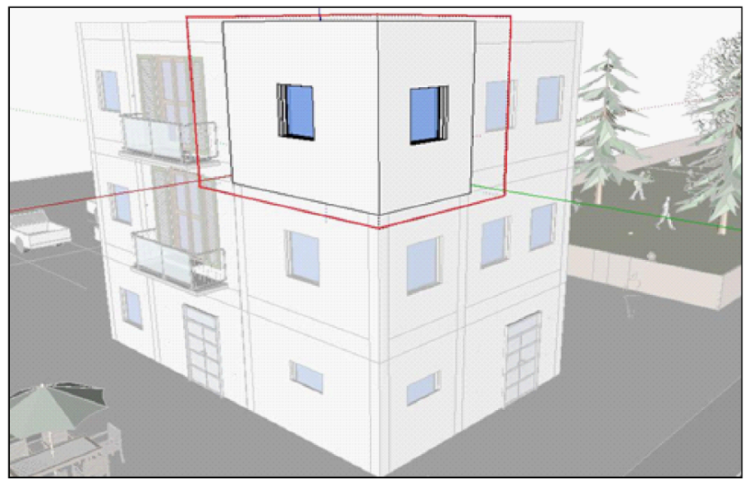
In order to prove the capability of the present numerical approach to integrate the behavior of 3D thermal bridges in the dynamic simulation of building structures, the geometry shown in
Figure 13 has been studied under transient conditions. This geometry represents the room of an apartment located at the top floor of a building, with two exterior walls and the roof exposed to the environment conditions. Two single-glass windows with an aluminum frame have been considered. The steel-concrete pillar studied in the previous section has been employed at the corners of this structure.
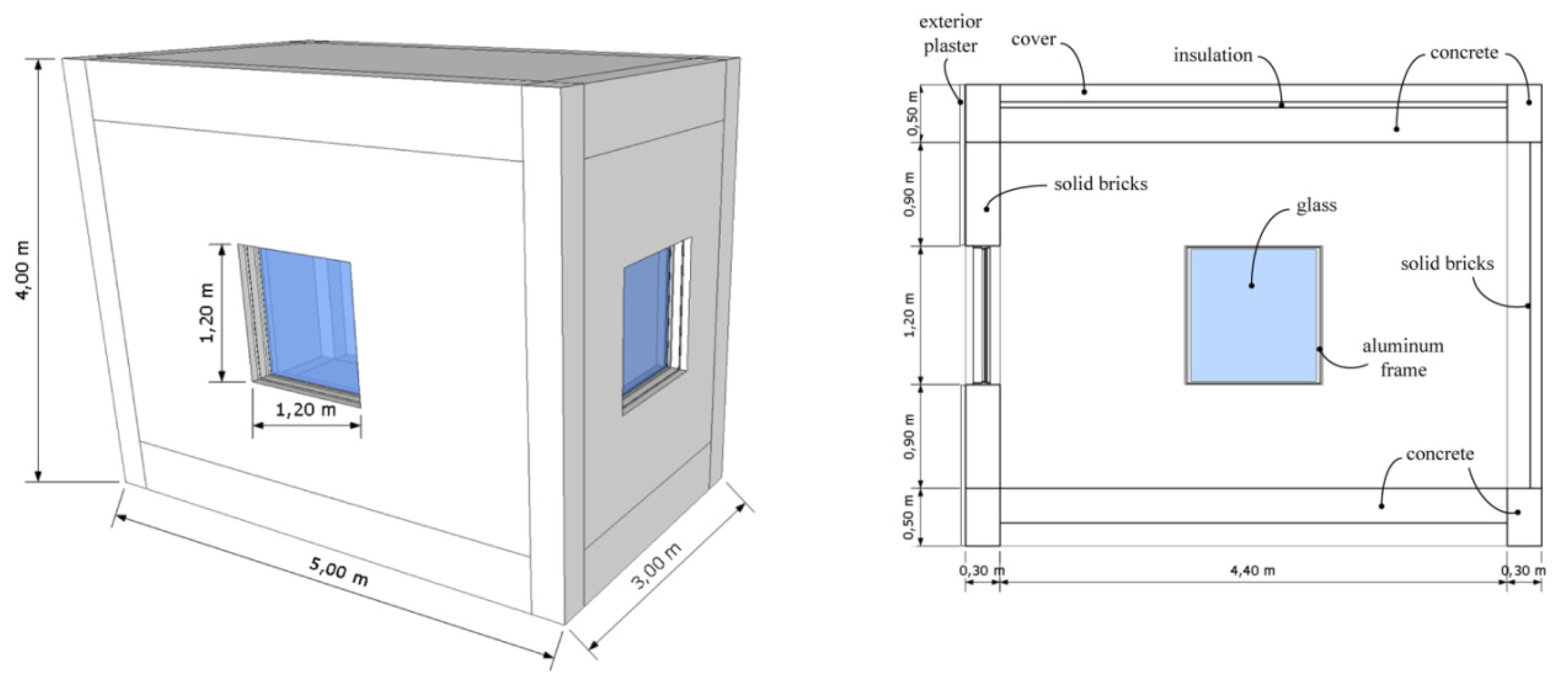
Figure 14 reports the geometric characteristics of the room envelope taken into account in the simulations. The exterior thermal boundary conditions are represented by Equations (11), including also radiative heat transfer on opaque surfaces, while Equation (12) represents exterior boundary conditions for vapor diffusion. A temperature of 20 °C, with a convective heat transfer coefficient equal to
, and a vapor partial pressure of 1168 Pa have been considered as boundary conditions at the interior of the room. Since the whole building has been considered at the same constant interior temperature and relative humidity and, as a consequence, partial pressure of vapor, the vertical wall without window and the pavement have been considered adiabatic and impermeable to mass.
This configuration could be considered representative of the actual behavior of a building envelope. In the authors’ opinion, the present 3D microscopic numerical approach should be used in order to evaluate local heat and mass transfer phenomena, while lumped parameter models could be used to reproduce the global behavior of building envelopes. The properties of the solid bricks, insulation material, concrete and plaster are those reported in
Table 3. As concerns the other materials used in the simulations carried out in this section, the physical properties, taken from the technical standard [
12], are reported in
Table 5.
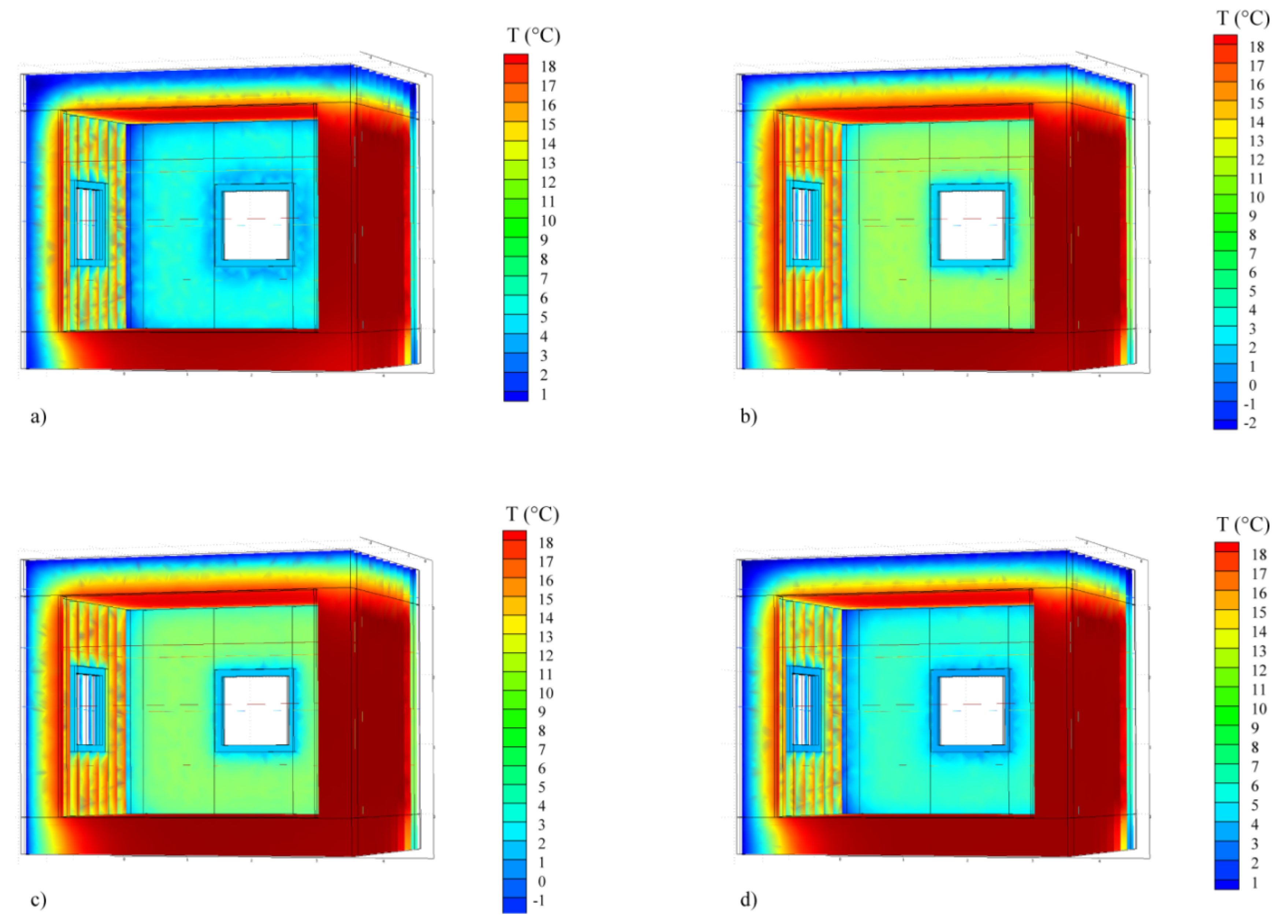
Figure 15 shows the temperature contours in the room envelope obtained at four different times (12, 48, 96 and 168 h). From the analysis of this figure, it is evident that the minimum temperatures of the interior side of the envelope are calculated in correspondence of the thermal bridges, and in particular at the corner between the exterior walls.
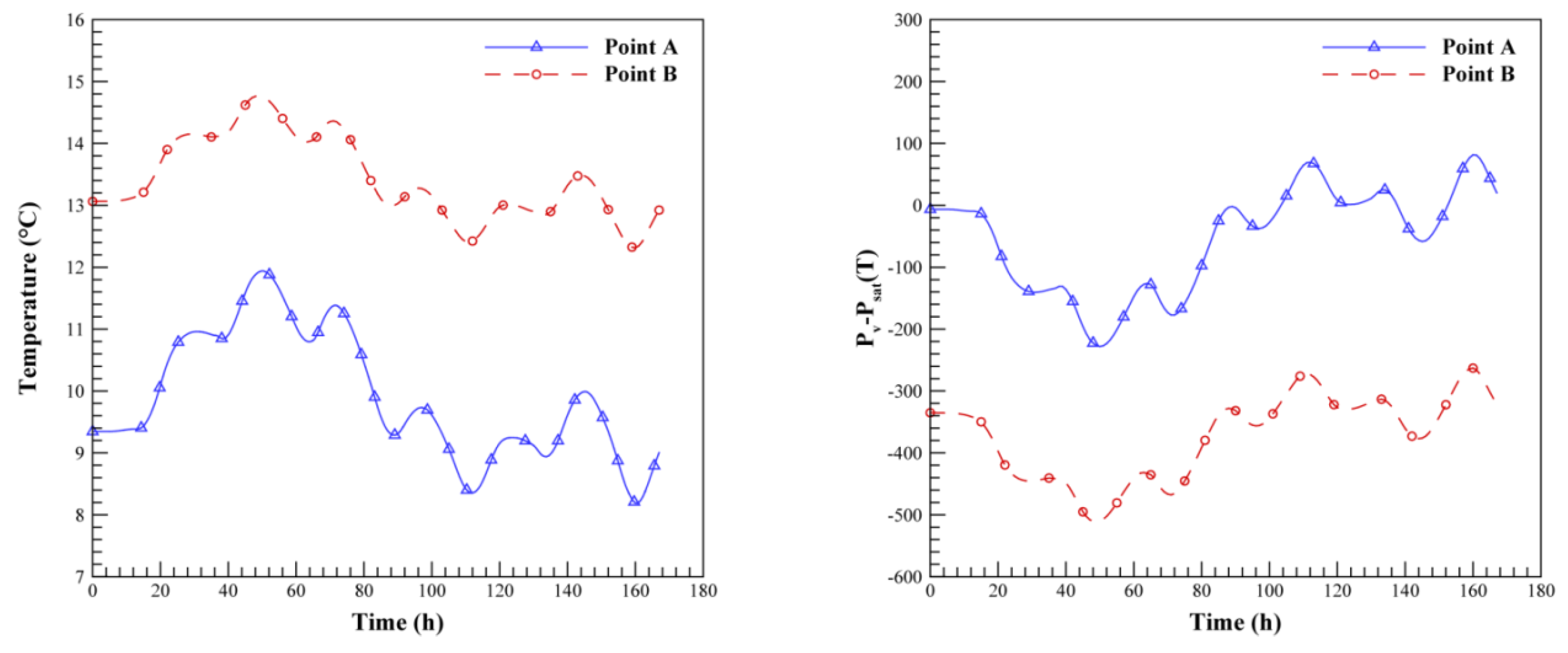
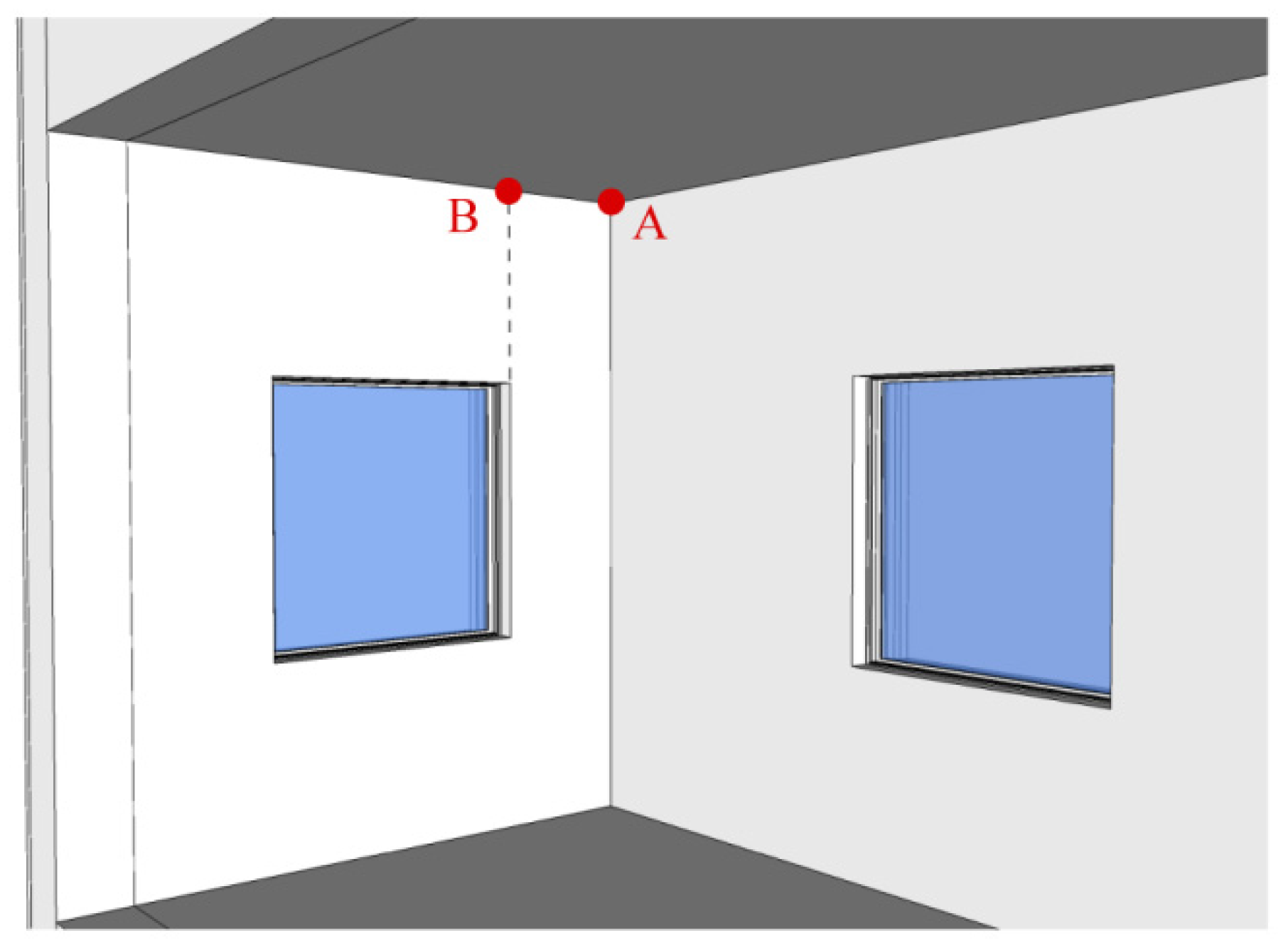
Figure 16 shows the variation of temperature and pressure difference over time at points A and B represented in
Figure 17. The results reported in
Figure 16 clearly show that the corner between walls, pillar and roof (point A) is the critical point of the envelope, as expected. In fact, the temperature values at point A are significantly smaller than those of point B during the whole week. As a consequence, the difference between partial pressure of vapor and saturation pressure of water assumes values greater than zero after about 105 h. This means that condensation occurs at the corner (point A), as expected, but not at point B.


