Article

Analysis and Modeling for China’s Electricity Demand Forecasting Using a Hybrid Method Based on Multiple Regression and Extreme Learning Machine: A View from Carbon Emission

1
School of Economics and Management, North China Electric Power University, Beijing 102206, China
2
College of Management and Economy, Beijing Institute of Technology, Beijing 100081, China
3
Department of Information Management, Oriental Institute of Technology, New Taipei 220, Taiwan
*
Author to whom correspondence should be addressed.
Energies 2016, 9(11), 941; https://doi.org/10.3390/en9110941
Submission received: 8 October 2016 / Revised: 3 November 2016 / Accepted: 4 November 2016 / Published: 11 November 2016

Abstract

:
The power industry is the main battlefield of CO2 emission reduction, which plays an important role in the implementation and development of the low carbon economy. The forecasting of electricity demand can provide a scientific basis for the country to formulate a power industry development strategy and further promote the sustained, healthy and rapid development of the national economy. Under the goal of low-carbon economy, medium and long term electricity demand forecasting will have very important practical significance. In this paper, a new hybrid electricity demand model framework is characterized as follows: firstly, integration of grey relation degree (GRD) with induced ordered weighted harmonic averaging operator (IOWHA) to propose a new weight determination method of hybrid forecasting model on basis of forecasting accuracy as induced variables is presented; secondly, utilization of the proposed weight determination method to construct the optimal hybrid forecasting model based on extreme learning machine (ELM) forecasting model and multiple regression (MR) model; thirdly, three scenarios in line with the level of realization of various carbon emission targets and dynamic simulation of effect of low-carbon economy on future electricity demand are discussed. The resulting findings show that, the proposed model outperformed and concentrated some monomial forecasting models, especially in boosting the overall instability dramatically. In addition, the development of a low-carbon economy will increase the demand for electricity, and have an impact on the adjustment of the electricity demand structure.

1. Introduction

As one of the leading pioneers of national economy advancement, the electricity sector shoulders the responsibility of ensuring a stable electricity consumption and economic expansion rapidly at home and abroad [1]. Relevant to the characteristics of the electric power commodity, such as instantaneous production, transport and consumption as well as non-storability, future power demand prediction seems imperative and inevitably required. Accordingly, such sort of prediction is beneficial to the entire electricity development planning process by allowing scientifically and timely adjustment of power demand variation conditions towards sustainability [2].
With the increasing attention to climate change and greenhouse gas (GHGs) emission abatement worldwide, China has initially attempted to extend a low-carbon economy pattern, namely in the pursuit of adoption of technical progress and institutional innovation to transform energy utilization patterns, enhance energy efficiency and optimize the energy sector structure [3]. Among GHGs forms, CO2 is on the top of list, accounting for 77% of global warming potential [4]. In China, CO2 emissions generated by fossil energy consumption not only account for approximately 80% of total global greenhouse emissions, but also account for more than two-thirds of the responsibility for adverse greenhouse effect [5,6]. This adverse effect is representative and deteriorates seriously China’ electricity sector. Regarding this, China has taken considerable countermeasures to address low-carbon issues, like climate deterioration, late environmental-protection starting of power sectors and so forth. In 2007, “Energy Saving Generation Dispatching” was published to decrease the carbon emission coefficient mainly caused by the thermal power structure [7]. Since 2013, much focus been placed on the emission-reducing effects of renewable energy sources, like zero release terms, and the National Development and Reform Commission (NDRC) in China has issued the so-called “12th five-year plan of renewable energy development” to further raise the proportion of renewable energy sources in the energy consumption mix to 15% [8] by 2020. As the largest emission-cutting participant in the clean development mechanism (CDM), China has obtained large emissions reductions from zealous participation and introduction of low-carbon technology and funds, whose checked emission reduction (CERs) reached 50% of the global share [9]. Generally, electricity demand forecasting research from the perspective of low-carbon economy proves much practical significance and practical value.
Currently, in the existing macroeconomic background, both domestic and international, numerous countries have selected appropriate variables and models to forecast electricity demand, such as Italy [10], Spain [11], USA [12], Brazil [13], Japan [14], Singapore [15], Thailand [16] and Indonesia [17]. In general, electricity demand forecasting methods can be decomposed into two aspects, namely traditional forecasting models and modern intelligent forecasting models. When it comes to traditional forecasting models, time series [18,19,20], regression analysis [21], Gray forecasting [22], fuzzy forecasting [23], index decomposition method [24] and so forth, are implemented widely. Pappas et al. [19,20] applied auto regressive moving average (ARMA) model to model the electricity demand loads in Greece, respectively using the Akaike corrected information criterion (AICC) and multi-model partitioning algorithm (MMPA). Hussain et al. [18] integrated Holt-winter with autoregressive integrated moving average (ARIMA) models on time series secondary data covering 1980–2011 in Pakistan, to predict overall and segmental electricity consumption. García and Carcedo [21] present an alternative analysis of electricity demand, on the basis of a simple growth rate decomposition scheme that allows vital factors behind this evolution to be identified. Similarly, Torrini et al. [22] employed the extended properties of fuzzy logic methodology to forecast the long-run electricity consumption in Brazil; while Zhao et al. [23] recommended an improved GM (1,1) model using Inner Mongolia as object. Further, multiple linear regression analysis and a quadratic regression analysis were performed deeply by Fumo et al. [24] on hourly and daily data from a research house. Inevitably, these traditional models have been comparatively proved to display a simple range of application and low-accuracy prediction thorough validated tools and simplified calculation. As for modern intelligent forecasting models, Günay [25] proposed artificial neural networks to forecast annual gross electricity demand using predicted values of social-economic indicators and climatic conditions. Son and Kim [26] applied support vector regression with particle swarm optimization algorithms to forecast the residential sector's electricity demand. Modern intelligent forecasting models have demonstrated excellent performance, including simplified regression course, transformation inference realization from training samples to predicted samples as well as avoidance towards the traditional process from induction to deduction [27]. However, they are easily trapped in over-fitting, local optima and so on. As a new type of single-hidden layer feedforward neural network primarily proposed by Huang et al. [28], extreme learning machine (ELM) embodies the features of adaptive ability, autonomic learning and optimal computation needed for unstructured and imprecise disciplines. Only by designing the suitable hidden layer nodes before training, bestowing value on input weight and partial hidden layer randomly in process, as well as simultaneously fulfilling at once without iterative, a sole optimum solution will be obtained.
Various forecasting models vary greatly from the perspective of distinct points to reflect economic variation tendencies, thus strengthening the weakness of lower accuracy using a single forecasting model. It was Bates and Granger [29] who firstly advocated combination forecasting approaches in 1969, and since then a considerable volume of studies have been conducted in many fields by domestic and overseas scholars [30,31,32]. The essence of combined forecasting is to solve the weighted average of single forecasting models. However, existing traditional combination forecasting models have fallen into a paralogism, namely different single forecasting models with distinguished weight coefficients, while constant combination models have unchanged weight coefficient [33]; in reality, the weight coefficient of a single forecasting model is supposed to be a function of time. Problems posed by traditional thought, are comprehensively conquered by the establishment of IOWHA operator-based forecasting models [34] in a concept of distinguished weight coefficients with the same single forecasting model over time [34,35]. Furthermore, the forecasting accuracy of the IOWHA operator shows an overdependence on the reciprocal error sum of squares which similarly is influenced by outliers to magnify the errors. Regarding this, the relevant properties of the grey relation degree (GRD) were devised and integrated with the IOWHA operator such as robust index combination, including dominance combination forecasting, non-pessimum forecasting and redundancy degree [36].
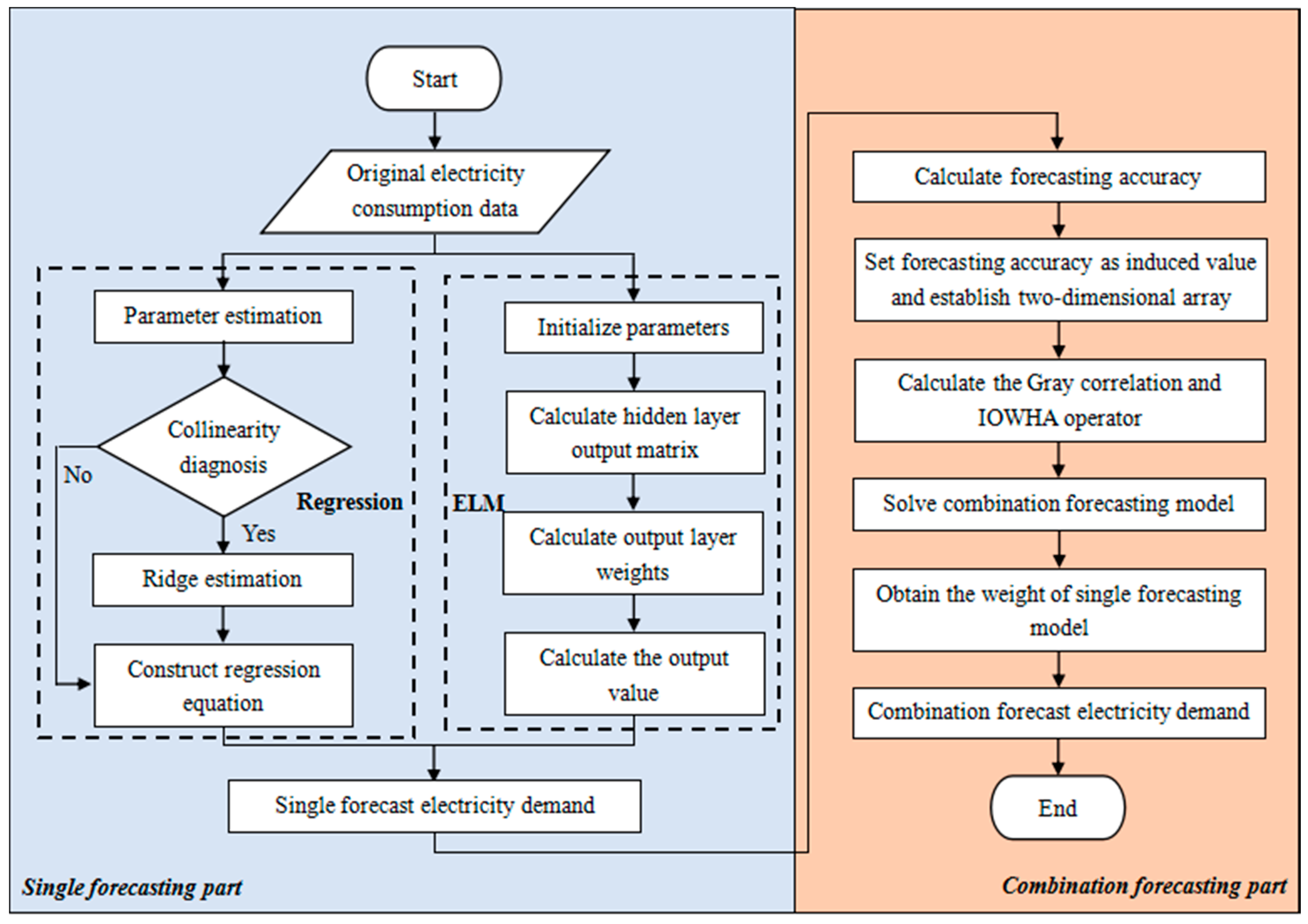
Hence, based on previous literature, a new framework of combination forecasting electricity demand model is characterized as follows: firstly, integration of GRD with the IOWHA operator to propose a new weight determination method of combination forecasting model on the basis of forecasting accuracy as induced variables; secondly, utilization of the proposed weight determination method to construct the optimal combination forecasting model based on the ELM forecasting model and multiple regression model; thirdly, three scenarios in line with the realization level of various low-carbon economy targets and dynamic simulation of the effects of low-carbon economy on future electricity demand. The remainder of this paper is organized as follows: Section 2 discusses low-carbon target scenario setting. In Section 3, a new combined GRD-IOWHA operator forecasting model is proposed. Section 4 and Section 5 discuss the combination forecasting model and model results of electricity demand in China, respectively. Overall conclusions are summarized in Section 6.

2. Low-Carbon Economy Simulation Scenarios

2.1. Variation Tendency Analysis of China’s Electricity Demand

By 2014, electricity consumption in China approached approximately 5626.31 million MW·h, which accounted for a quarter of world’s total electricity consumption and ranked the first. Thus, electricity demand of China is representative and outperformed in terms of both applicability and feasibility.
As Figure 1 depicts (the data is sourced from the China Statistical Yearbook), in 2000–2014, the annual electricity demand of China enjoyed stable and relatively fast growth, with an average annual growth rate of 10.82%; During that period, the steepest increasing emerged in 2003, with a growth rate of 16.53%. From 2000 to 2007, electricity demand still maintained a high upward trend at an average growth rate of 13.54%; meanwhile, power demand in 2008–2009 slowed down, especially for export-oriented areas (such as East China and Guangdong at merely 5.59% and 7.21%) due to several constraint factors, including the crunch in domestic credit, Renminbi (RMB) appreciation, changes in international market demand, adjusted import-export policy, and regulatory resources, climate change, etc.
Along with the comprehensive implementation of “12th Five-Year Program”, China has been accelerating the shifting in economic growth model to achieve sound and fast economic growth, together with attempts to support strategic emerging industries and upgrade traditional industries. Subsequently, the continuously adjusted consumption structure has curbed the excessive expansion of the heavy energy-consuming industry (including chemical industry, building materials, black metal smelting and smelting non-ferrous metal) and suppress China’s electricity demand at a lower level. Typically in 2014, China shows a year-on-year electricity demand growth of 3.8% together with a year-on-year growth rate drop 5.12%. Under the existence of multiple uncertainties, electricity demand prediction is worthy of further exploration for prospective programming.

2.2. Scenario Mode

With the objective to clarify the effect of energy-efficient and emission-cutting constraints on future electricity demand, three scenarios are set here to dynamically simulate future electricity demand forecasting:
(1)
Baseline scenario mode. Under this mode, electricity demand growth is stimulated by economic advancement and booming population in the direction of a scheduled economic growth rate of a moderately prosperous society and population progress the same as usual.
(2)
Low-carbon scenario mode. Low-carbon mode is aimed at fulfilling emission-reducing responsibilities promised during international climate talks and simultaneously promoting economic advancement by technical progress, industrial restructuring and so forth. Excluding the impact factors of economic development and population growth, electricity demand is also restrained by carbon emissions quotas.
(3)
Intensified low-carbon scenario mode. Along with the thorough implementation of energy-conserved and emission-reducing policies and economic development pattern transformation towards three-low issues (low consumption, low emissions and low pollution), a low-carbon economy is well achieved by converted energy utilization patterns, enhanced energy efficiency, adjusted energy structures and so on. In this intensified mode, electricity demand is largely influenced by economic development, population growth, policy constraint and so forth.

2.3. Scenario Parameter Setting

In views of factor diversity and variability, there is a necessity to elaborate future development trend of electricity demand impact factors especially in a mid-and long term. Numerous factors are involved in China’s electricity demand variation, such as economic development level, electricity price, population growth and policy constraint [24,25,26,27,28,29,30,31,32]. While considering the data availability and typicality, this paper merely took into account of gross domestic product (GDP), booming of the population and energy policy constraints (specifically explained in Section 2.3.3), described in Table 1.

2.3.1. Economic Development Level and Population

(1) GDP. Here GDP is chosen to represent economic development level. According to deepening target released in the 18th national congress of the communist party of China [37], GDP will double by 2020 with an annual growth rate at 7% roughly. Table 2 and Figure 2 illustrated GDP growth by 2020.
(2) Population growth. Based on constraint conditions, population forecasting variables mainly adopted direct influential parameters, like birth rate, death rate and mobility ratio. Empirical model can be interpreted as:
N t = N t 0 e k ( t t 0 )
where Nt means gross population at t; is the population base at t = t0; k denotes natural population growth rate; e is the base of natural logarithms (e = 2.718). In line with the stable natural population growth rate over 2009–2014, we assume k = 4.92‰. Besides, population base is set as gross population in 2014, namely =13.68.

2.3.2. Electricity Price

Due to inexhaustive electric power system reformation and an immature electricity market, electricity price is determined by governmental macroeconomic regulation rather than an open market. Thus electricity price is failed to be predicted and ignored.

2.3.3. Energy Policy

Policy on energy conservation and emission reduction have energetically affected China’s electricity demand variation and provided a more explicit target. Here CO2 emissions per GDP and energy consumption per GDP are picked as explained variables:
Energy consumption per GDP = Gross primary energy consumption ÷ GDP
CO 2   emissions of primary energy at i = Primary energy consumption at i × CO 2   emissions factor
where primary energy includes coal, oil, natural gas and nuclear power, hydropower, wind power and so on; According to the National Development and Reform Commission Energy Research Institute in 2003, CO2 emission factors of coal, oil, natural gas, nuclear power, hydropower and wind power are separately 0.7476, 0.582 5, 0.443 5, 0, 0 and 0 [38]. From the requirements of the 13th Five Year Plan [39], up to 2020, CO2 emissions per GDP and energy consumption per GDP are reduced by 18% and 15% respectively. This study chooses the average value of 2015, namely CO2 emissions per GDP at 3.6% and energy consumption per GDP at 3%, and then calculates their values in 2020, as Table 2 and Figure 2.

3. Combination Forecasting Model of Electricity Demand Using GRD-IOWHA Operator

3.1. Regression Analysis

3.1.1. Multiple Linear Regression

Multiple linear regression, aiming at investigating the linear relationship between dependent variable and multiple independent variables, is written as below [40]:
Y = β 0 + β 1 X 1 + β 2 X 2 + β 3 X 3 + + β j X j + + β k X k + ε
where k is the quantity of explanatory variable; βj (j = 1,2,…,k) means regression coefficient; ε denotes the random error after eliminating the effect of independent variables on Y. Stochastic equations can be expressed as Equation (3). Besides, if X is column full rank, ordinary least squares estimate could be adopted to Equation (3), boiled down to Equation (4):
Y = X β + ε
β ^ = ( X X ) 1 X Y

3.1.2. Ridge Regression

Serious multicollinearity may lead to the failure of regression models, thus providing invalid results. Ridge regression has been exclusively used to eliminate multicollinearity by abandoning unbiasedness of least square method [41]. For the linear regression model in Equation (3), regressed parameter β can be transformed as [39]:
β ^ ( k ) = ( X X + k I ) 1 X Y
where k > 0 is ridge parameter. Varies greatly from various k, thus deeming as estimator clan. Estimator clan can be drawn by a portrait of along the k.

3.2. Extreme Learning Machine (ELM)

Different from a traditional feed forward neural network, ELM uses a non-iterative hidden layer, random selection of input weight and node and successive computed-output weight. ELM is aimed at achieving minimum training error. Excitation function G, having hidden layer N is interpreted as [28]:
f N ¯ = i = 1 N ¯ β i G ( a i , b i , x j ) = t j j = 1 , 2 , , N
where a i = [ a 1 , a 2 , , a n ] T is the weight vector of hidden node i; β i = [ β 1 , β 2 , , β n ] T means the weight vector of input node and output node; bi is polarization of node i; denotes hidden node quantity. For simplicity, Equation (6) is transformed as:
H β = T
H ( a 1 , , a N ¯ , b 1 , , b N ¯ , x 1 , , x N ) = [ G ( a 1 , b 1 , x 1 ) G ( a N ¯ , b N ¯ , x 1 ) G ( a 1 , b 1 , x N ) G ( a N ¯ , b N ¯ , x N ) ] N N ¯
{ β = [ β 1 T , , β N ¯ T ] N ¯ m T = [ t 1 T , , t N T ] N m
where H means output matrix of hidden layer. Output weight can be obtained from least square solution Equation (11) of Equation (10):
H β T = H H + T T = min β H β T
β = H + T
where H+ is Moore-Penros generalized inverse matrix of .

3.3. IOWHA Operator

Supposing u 1 , a 1 , u 2 , a 2 , , u n , a n as two-dimensional array, W = ( w 1 , w 2 , , w n ) T means a weighted vector related to Hw, and i = 1 n w i = 1 . By definition, Hw points to induced ordered weighted harmonic averaging (IOWHA) operator [35] as Equation (12):
H w ( u 1 , a 1 , u 2 , a 2 , , u n , a n ) = 1 / i = 1 n w i a u i n d e x ( i )
where ui is the induced value of ai; uindex(i) denotes the subscript of ui. Weight coefficient wi has nothing to do with position and size of ai, but position of its induced value.

3.4. IOWHA Operator-Based Combination Forecasting Model

Among existence of m kinds of single forecasting models, we assume xit as the forecasting value of i at t and suppose l1,l2,…,lm as the weighted coefficient of single forecasting models in combination forecasting:
a i t = { 1 | ( x t x i t ) / x t | ,   | ( x t x i t ) / x t | < 1 0 ,   | ( x t x i t ) / x t | 1 , i = 1 , 2 , , m ,   t = 1 , 2 , , N
where ait means the forecasting accuracy of model i at t; i = 1,2,…,m; t = 1,2,…,N.
Taken forecasting accuracy ait as induced value of xit, assumed a 1 t , x 1 t , a 2 t , x 2 t , , a m t , x m t as a two-dimensional array of m and arranged forecasting accuracy a1t,a2t,…,amt, then Equation (14) is summarized, termed as IOWHA operator-based combination forecasting value by a1t,a2t,…,amt:
x ^ t = H ( a 1 t , x 1 t , a 2 t , x 2 t , , a m t , x m t ) = 1 / i = 1 m l i x a i n d e x ( i t ) , t = 1 , 2 , , N
In average combination forecasting, time series is processed by selecting reciprocal error for convenience. S, reciprocal error sum squares of IOWHA operator-based combination forecasting, is written in Equation (15). Abridged weighting coefficient vector of single forecasting methods as, then we can transform Equation (15) into Equation (16) [5]:
S = t = 1 N ( 1 x t 1 x ^ t ) 2 = t = 1 N ( i = 1 m l i ( 1 x t 1 x a i n d e x ( i t ) ) ) 2 = i = 1 m j = 1 m l i l j ( t = 1 N e a i n d e x ( i t ) e a i n d e x ( j t ) )
where e a i n d e x ( i t ) = 1 x t 1 x a i n d e x ( i t ) .
min S ( L ) = i = 1 m j = 1 m l i l j ( i = 1 N e a i n d e x ( i t ) e a i n d e x ( j t ) ) s . t . { i = 1 m l i = 1 l i 0 , i = 1 , 2 , , m

3.5. GRD-IOWHA Operator-Based Combination Forecasting Model

IOWHA operator-based combination forecasting model, usually exploits reciprocal error sum of squares to reflect forecasting accuracy. While, reciprocal error sum of squares is easily influenced by outliers thus leading to error amplification. Regarding this, grey relation degree (GRD) is introduced to maintain robust forecasting.
Both sides of Equation (14) are handled by reciprocal like Equation (17):
1 x ^ = i = 1 m l i x a i n d e x ( i t ) ,   t = 1 , 2 , , N
Seen from Equation (17):
min 1 i m 1 x i t = min 1 i m 1 x a i n d e x ( i t ) 1 x ^ max 1 i m 1 x a i n d e x ( i t ) = max 1 i m 1 x i t ,   t = 1 , 2 , , N
et is assumed as the reciprocal error between combination forecasting value and actual value at t, therefore Equation (19) appears. We can call Equation (20) GRD of reciprocal series between single forecasting method forecasting values and real values of i. Likely, Equation (21) is named the GRD of reciprocal series between IOWHA operator-based forecasting value and real values of i.
e t = 1 x t 1 x ^ t = i = 1 m l i 1 x t i = 1 m l i 1 x a i n d e x ( i t ) = i = 1 m l i ( 1 x t 1 x a i n d e x ( i t ) ) = i = 1 m l i e a i n d e x ( i t )
γ i = 1 N t = 1 N min 1 i m min 1 t N | e i t | + ρ max 1 i m max 1 t N | e i t | | e i t | + ρ max 1 i m max 1 t N | e i t |
γ = 1 N t = 1 N min 1 i m min 1 t N | e i t | + ρ max 1 i m max 1 t N | e i t | | e t | + ρ max 1 i m max 1 t N | e i t |
where e i t = 1 / x t 1 / x i t means the reciprocal errors between forecasting values and real values of i and ρ ( 0 , 1 ) is the resolution coefficient, usually at 0.5.
Based on Equation (19), GRD of reciprocal series between combination forecasting values and actual values, i.e., γ can be rewritten as below:
γ = 1 N t = 1 N min 1 i m min 1 t N | e i t | + ρ max 1 i m max 1 t N | e i t | | i = 1 m l i ( 1 x t 1 x a i n d e x ( i t ) ) | + ρ max 1 i m max 1 t N | e i t |
where γ is the function of weighting coefficient vector of single forecasting model, called γ(L). A higher γ, the more effective combination forecasting model will be. Hence, IOWHA operator-based combination forecasting model is summarized as:
max γ ( L ) = 1 N t = 1 N min 1 i m min 1 t N | e i t | + ρ max 1 i m max 1 t N | e i t | | i = 1 m l i ( 1 x t 1 x a i n d e x ( i t ) ) | + ρ max 1 i m max 1 t N | e i t | s . t . { i = 1 m l i = 1 l i 0 , i = 1 , 2 , , m
Plugging into Equation (24) to perform GRD-IOWHA operator-based combination forecasting:
x ^ t = H ( a 1 t , x 1 t , a 2 t , x 2 t , , a m t , x m t ) = 1 / i = 1 m l i * x a i n d e x ( i t ) ,   t = N + 1 , N + 2 , ,
where during interval [N+1,N+2,…,], the size of forecasting accuracy series a1t,a2t,…,amt, is determined by the distance to average fitting accuracy. In other words, the forecasting accuracy in interval N + k is substituted by average fitting accuracy 1 / k t = N k + 1 N a i t of step k.
Regression analysis is termed as RA, while grey relation degree and modified IOWHA operator is short for GRD-IOWHA operator. Thus far, based on modified GRD-IOWHA operator, combination forecasting modeling is constituted by multiple regression as well as ELM, and completely fulfilled. Figure 3 depicts the operational process concretely, where the left demonstrates two single forecasting modeling and the right explains combination forecasting modeling.

4. Electricity Demand Forecasting in China

This section took full advantage of the above-proposed combination forecasting model to predict China’s electricity demand under three types of low-carbon scenarios. Among that, for MR forecasting, we use data in 2000–2008 to simulate and data in 2009–2014 to test. The same occurs for ELM, where training sample is derived from data in 2000–2008, and test sample is from 2009–2014.

4.1. Baseline Scenario Forecasting

4.1.1. Forecasting of RA and ELM

Let GDP be x1 and population be x2, linear regression model is boiled down to the following:
y = 427.31 x 1 + 21559.93 x 2 264862.86
Deduced from calculation, modified fitting degree R2 = 0.997. Moreover, in the significance level of α = 0.05, statistics F = 2406.802 > F0.05(2,12) = 2.81 and each statistics T > t0.025(12) = 2.179, respectively, which means that regressed model has passed significance testing and embodies a better imitative effect. Table 3 and Table 4 separately discussed test process using data from 2009–2014 and single forecasting covering data from 2015–2020.
Referencing the achievements of Huang et al. [28], this paper adopted the Matlab software to compile the ELM toolkit, together with the “Sigmoid function” to activate neurons in the hidden layer. The number of neurons of the hidden layer is set at 9. As for ELM forecasting in Table 3, data covering 2000–2008 is plugged in for training and data in 2009–2014 to test the well-trained model; Then, single forecasting of China’s electricity demand in 2015–2020 is carried out, as shown in Table 4.

4.1.2. GRD-IOWHA Forecasting

Two single forecasting results are exploited to construct forecasting accuracy and relevant in sample interval, t = 1,2,…,6. The IOWHA operator-based forecasting value is displayed as below:
x ^ 1 = H ( a 11 , x 11 , a 21 , x 21 ) = 1 / ( l 1 / 36680.39 + l 2 / 37730.04 )
x ^ 2 = H ( a 12 , x 12 , a 22 , x 22 ) = 1 / ( l 1 / 41728.51 + l 2 / 42509.00 )
x ^ 3 = H ( a 13 , x 13 , a 23 , x 23 ) = 1 / ( l 1 / 47442.71 + l 2 / 46235.47 )
x ^ 4 = H ( a 14 , x 14 , a 24 , x 24 ) = 1 / ( l 1 / 49881.22 + l 2 / 48473.75 )
x ^ 5 = H ( a 15 , x 15 , a 25 , x 25 ) = 1 / ( l 1 / 53693.62 + l 2 / 53276.52 )
x ^ 6 = H ( a 16 , x 16 , a 26 , x 26 ) = 1 / ( l 1 / 55908.64 + l 2 / 57258.17 )
where l1 and l2 show weighting coefficients of two single forecasting models in combination forecasting.
With its direct substitution into Equation (23), the most effective weight coefficient of combination forecasting model is expressed as below with ρ = 0.5.
l 1 * = 0.7325 , l 2 * = 0.2675
Taking the average accuracy of former 6 as each single forecasting accuracy, we can obtain the combination forecasting results of China’s electricity demand in baseline scenario covering 2015–2020, shown in Table 5.

4.2. Low-Carbon Scenario Forecasting

4.2.1. Forecasting of RA and ELM

In order to eliminate the multicollinearity of selected variables, the low-carbon scenario and intensified scenario necessarily employed ridge regression to achieve efficient fitting. Similarly, let GDP be x1, population be x2 and CO2 emissions per GDP be x3. Besides, take the logarithm term to remove variable heteroscedasticity. SPSS 20.0 software was used to conduct the ridge regression shown in Figure 4 and Figure 5.
From the ridge trace, when K is nearly close to 0.2, all parameters tend to be stable; Even when K exceeds 0.2, the determination coefficient presents a stable decline without drastic fluctuation. Setting K = 0.2 and R2 = 0.9709, the ridge regression model is fitted as follows:
ln   y = 0.28 ln   x 1 + 7.86 ln   x 2 0.27 ln   x 3 10.98
In the significance level of α = 0.05, statistics F = 156.913 > F0.05(3,12) = 2.61 and each statistics T > t0.05(12) = 2.179 all demonstrated that regressed model had passed through significance testing with a well-fitting level, as shown in Table 6 and Table 7. Results of ELM method forecasting are shown there also.

4.2.2. GRD-IOWHA Operator-Based Combination Forecasting

Iterative steps like above-mentioned, GRD-IOWHA operator-based combination forecasting is summarized as below:
x ^ 1 = H ( a 11 , x 11 , a 21 , x 21 ) = 1 / ( l 1 / 36540.79 + l 2 / 37683.97 )
x ^ 2 = H ( a 12 , x 12 , a 22 , x 22 ) = 1 / ( l 1 / 42408.36 + l 2 / 40878.39 )
x ^ 3 = H ( a 13 , x 13 , a 23 , x 23 ) = 1 / ( l 1 / 47461.51 + l 2 / 45390.34 )
x ^ 4 = H ( a 14 , x 14 , a 24 , x 24 ) = 1 / ( l 1 / 49709.48 + l 2 / 50265.20 )
x ^ 5 = H ( a 15 , x 15 , a 25 , x 25 ) = 1 / ( l 1 / 53914.26 + l 2 / 55531.38 )
x ^ 6 = H ( a 16 , x 16 , a 26 , x 26 ) = 1 / ( l 1 / 56893.25 + l 2 / 58759.43 )
With utilization of the optimal tool in the Matlab software, the combination forecasting model shows the most powerful coefficient, are shown as below. Future electricity demand in China is predicted in Table 8.
l 1 * = 0.6981 , l 2 * = 0.3019

4.3. Forecasting in Reinforced Low-Carbon Scenario

4.3.1. Forecasting of RA and ELM

Likewise, let GDP be x1, population be x2 and CO2 emissions per GDP be x3, energy consumption per GDP be x4. Taking variables in logarithm terms, the ridge trace and K variation are displayed in Figure 6 and Figure 7.
Based on ridge trace, when K is nearly close to 0.2, all parameters tend to be stable; Even when K exceeds 0.2, the determined coefficient presents a stable declination without drastic fluctuation. Setting K = 0.2 and R2 = 0.9623, the ridge regression model is fitted as follows:
ln   y = 0.25 ln   x 1 + 7.29 ln   x 2 0.18 ln   x 3 0.22 ln   x 4 9.36
In the significance level of α = 0.05, statistics F = 90.430 > F0.05(3,12) = 2.61 and each statistics T > t0.05(12) = 2.179 all demonstrated that the regressed model had passed through significance testing with a well-fitting level, as shown in Table 9 and Table 10. Also, like the previous scenario’s parameter setting, test results and forecasting results of ELM method are shown here.

4.3.2. GRD-IOWHA Operator-Based Combination Forecasting

Similar forecasting process to above-mentioned section, IOWHA operator-based combination forecasting results display as below:
x ^ 1 = H ( a 11 , x 11 , a 21 , x 21 ) = 1 / ( l 1 / 36565.66 + l 2 / 36295.26 )
x ^ 2 = H ( a 12 , x 12 , a 22 , x 22 ) = 1 / ( l 1 / 42639.00 + l 2 / 41044.15 )
x ^ 3 = H ( a 13 , x 13 , a 23 , x 23 ) = 1 / ( l 1 / 47673.01 + l 2 / 45822.55 )
x ^ 4 = H ( a 14 , x 14 , a 24 , x 24 ) = 1 / ( l 1 / 50249.02 + l 2 / 50270.18 )
x ^ 5 = H ( a 15 , x 15 , a 25 , x 25 ) = 1 / ( l 1 / 54581.74 + l 2 / 54837.58 )
x ^ 6 = H ( a 16 , x 16 , a 26 , x 26 ) = 1 / ( l 1 / 57697.81 + l 2 / 59514.14 )
With utilization of optimal took it in Matlab software, combination forecasting model shows the most powerful coefficient, shown as below. Future electricity demand in China is predicted in Table 11.
l 1 * = 0.6459 , l 2 * = 0.3541

5. Results and Discussions

Deduced from China’s electricity demand forecasting results under various scenarios, further discussion is concluded from four perspectives.
(1) GRD-IOWHA operator-based combination forecasting model outperformed each single forecasting model notably. 
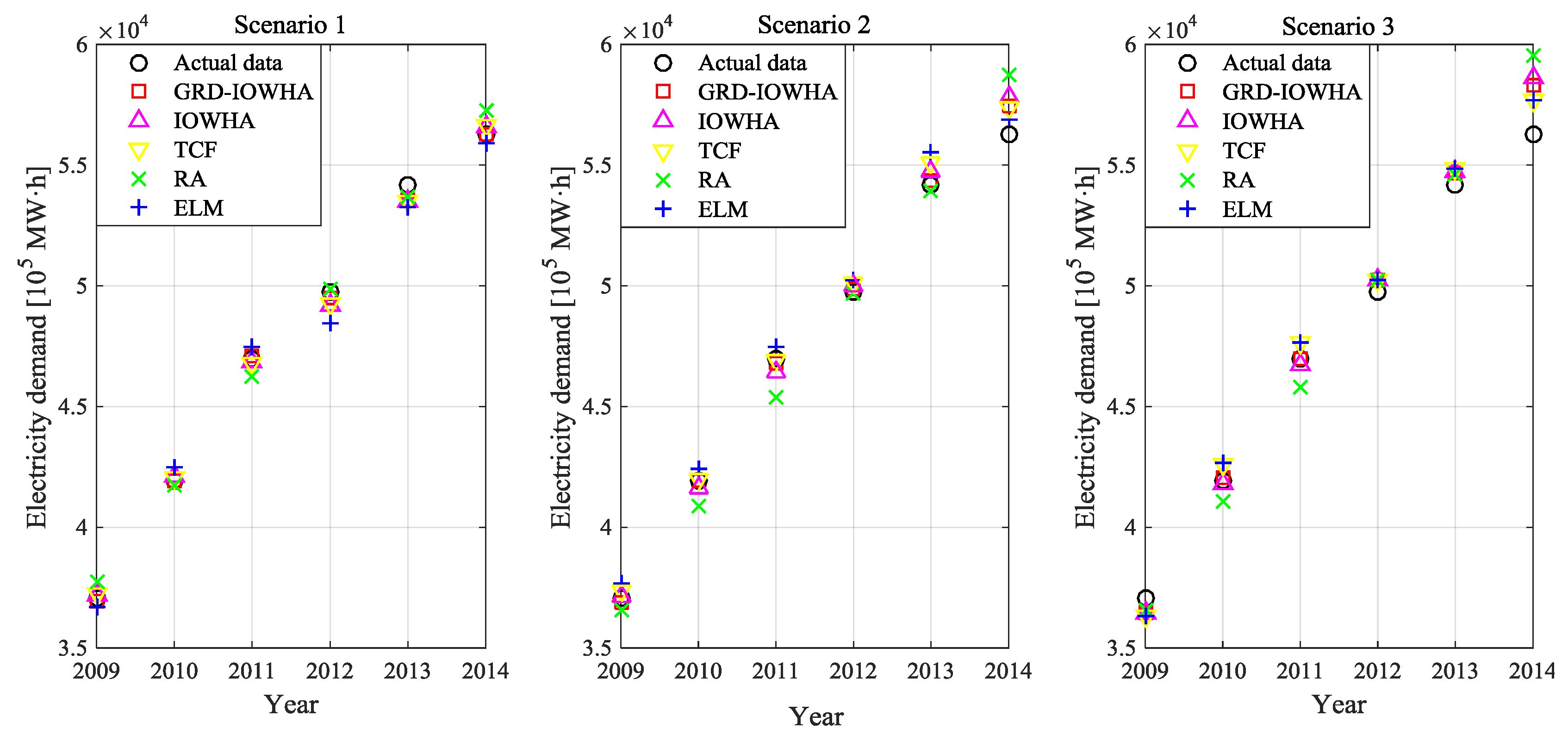
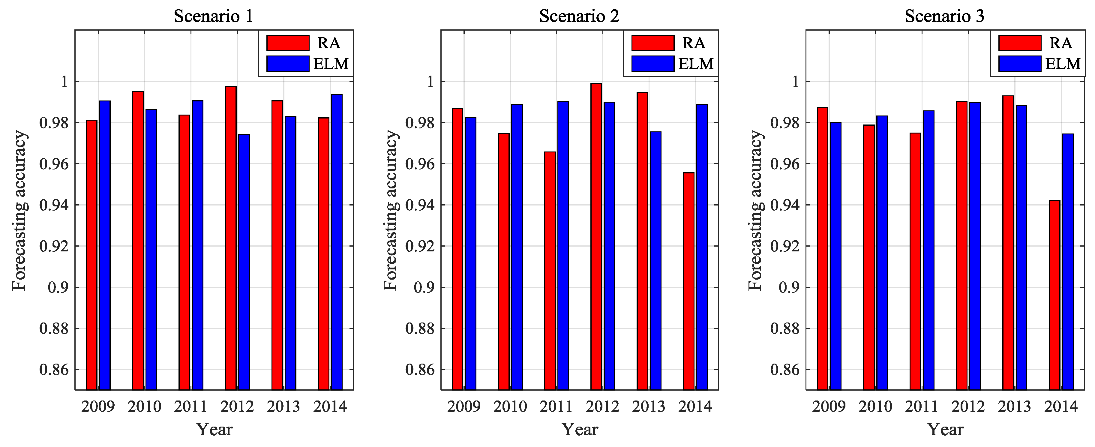
Figure 8 demonstrates the forecasting accuracy comparison of single forecasting models covering testing data in 2009–2014, where Scenario 1 means baseline scenario, Scenario 2 represents the low-carbon scenario and Scenario 3 in the intensified low-carbon scenario. Single forecasting models provide various forecasting accuracy at various moments. More specifically, in the baseline scenario, the ELM model shows a superior forecasting accuracy of electricity demand than the RA model in 2009, 2011 and 2014; while the RA model is much better in 2010, 2012 and 2013. In the low-carbon scenario, the RA model provides better forecasting accuracy than the ELM model, namely 2009, 2012 and 2013; while the ELM model predicts electricity demand overwhelmingly in other years (2010, 2011 and 2014). In the intensified low-carbon scenario, the RA model provides higher forecasting accuracy in 2009, 2012 and 2013 and lower forecasting accuracy in 2010, 2011 and 2014. Generally, the proposed GRD-IOWHA operator-based combination forecasting model concentrates the advantages of various single forecasting models, namely higher weight coefficient in higher single forecasting accuracy and vice versa. According to Equations (20) and (21), Table 12 represents grey relation degree comparison, from 2009 to 2014, in various scenarios between single forecasting model and GRD-IOWHA operator-based combination forecasting model. Findings show that grey relation degree of three scenarios in GRD-IOWHA operator-based combination forecasting model is better than that of single forecasting models. Thus, the proposed combination model belongs to the dominated forecasting combination model [36].
(2) The proposed GRD-IOWHA operator-based combination forecasting model predicts accurately and more truly than the basic IOWHA operator-based combination forecasting model [35] and the traditional combination forecasting (TCF) model [33], namely each single forecasting model with unchanged weight coefficient. In order to compare typical combination forecasting models effectively, this section compares the measured IOWHA operator-based combination forecasting model and traditional combination models shown in Table 13.
According to the evaluating principle of forecasting effect, the following dimensions are selected as the evaluation index system, including RE, SSE, MSE, MAE, MAPE, MSPE. Concretely, only RE is used to reflect single forecasting model effect. Figure 9 illustrates electricity demand forecasting in 2009–2014 using GRD-IOWHA operator-based combination forecasting model, IOWHA operator-based combination forecasting model and traditional combination forecasting model separately:
Relative error :   R E = ( x ^ t x t ) / x t
Error of sum square :   S S E = t = 1 N ( x t x ^ t ) 2
Mean square error :   M S E = 1 N t = 1 N ( x t x ^ t ) 2
Mean absolute error :   M A E = 1 N t = 1 N | x t x ^ t |
Mean Absolute Percentage Error :   M A P E = 1 N t = 1 N | ( x t x ^ t ) / x t |
where xt denotes the actual demand value, presents the predicted value.
Compared with the other forecasting models, the proposed GRD-IOWHA operator-based combination forecasting model is rather close to actual values. From 
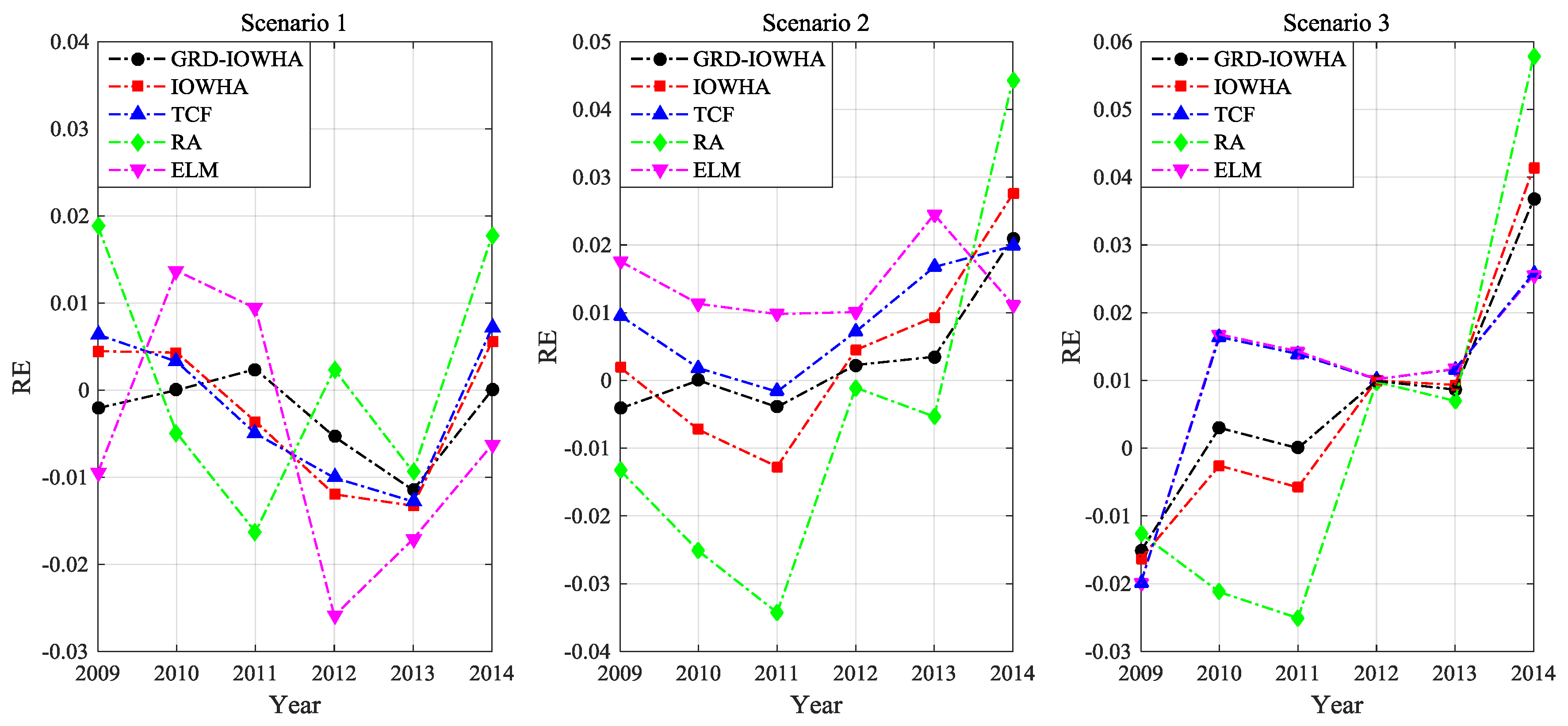
Figure 10, under the distinguished scenario, the relative error value of the proposed GRD-IOWHA operator-based combination forecasting model is in much lower interval and fluctuates slightly, followed by IOWHA operator-based combination forecasting model or traditional combination forecasting model, worst in two single forecasting model. In a word, proposed GRD-IOWHA operator-based combination forecasting model perform more superiority in decreasing forecasting error fluctuation and risk of tech-economic decision making. Furthermore, 
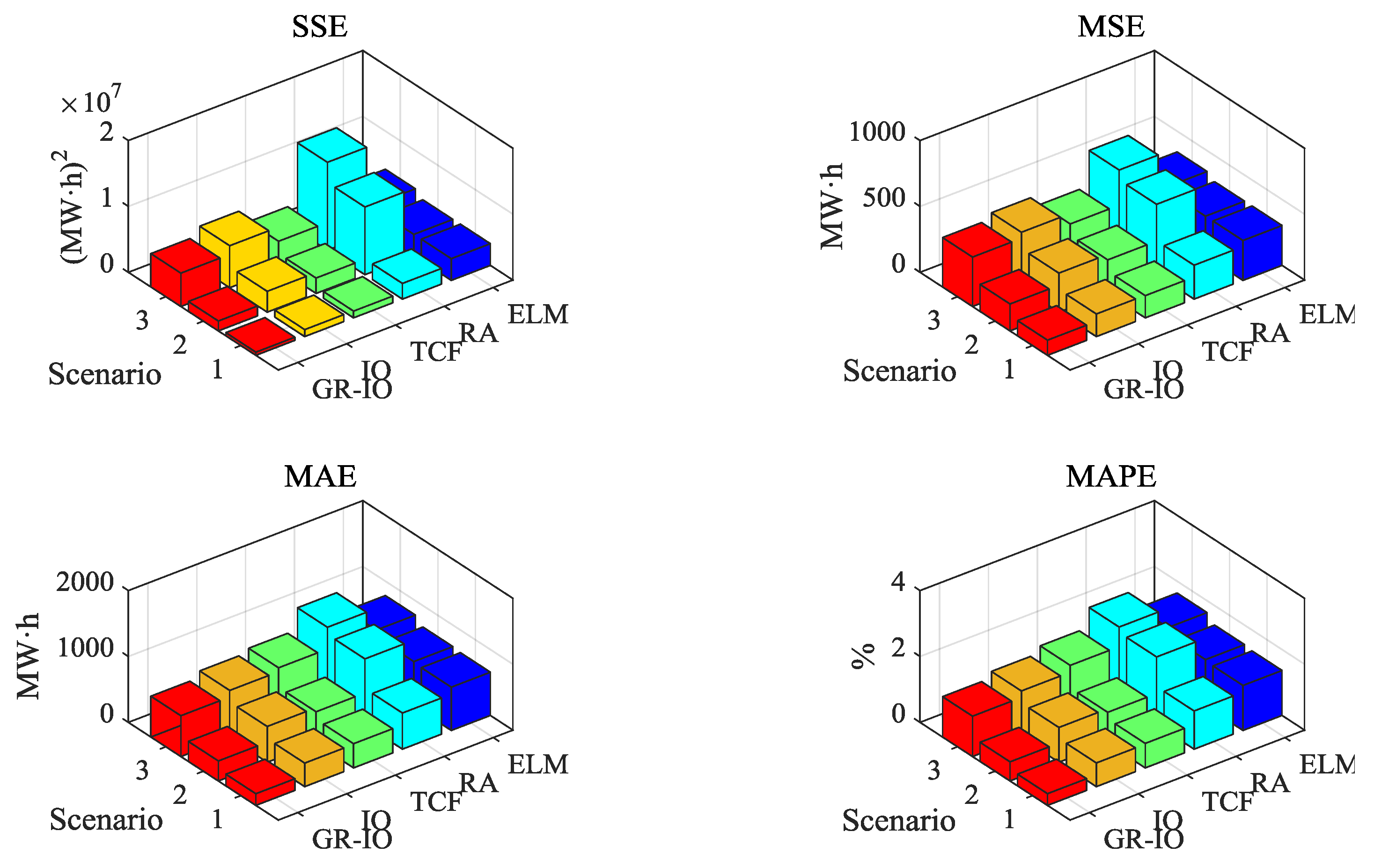
Figure 11 demonstrates the overall forecasting evaluation result of various forecasting model, especially being satisfactory and optimal condition in index SSE, MSE, MAE and MAPE. Yet exceptional situations still exist, like lower SSE and MSE in a traditional forecasting model than the GRD-IOWHA operator-based combination forecasting model under intensified low-carbon scenario due to larger forecasting error caused by single forecasting models. In spite of this, the proposed combination forecasting model outperformed both in effectiveness and feasibility as a whole.
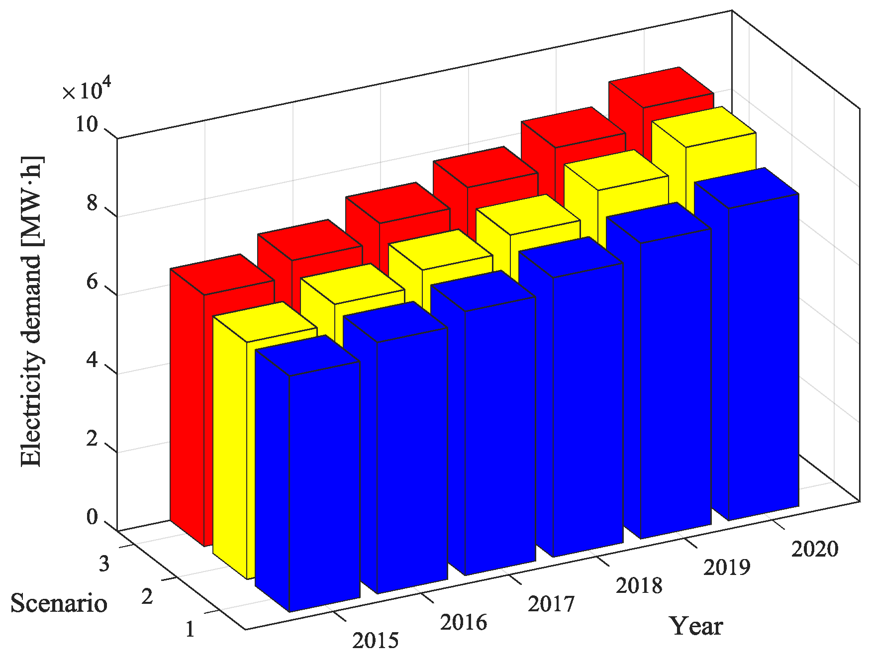
(3) Low-carbon economy advancement contributes to augment electricity demand in China. Known from Figure 12, electricity demand under energy restriction, i.e., low-carbon scenario and intensified low-carbon scenario, is greater than that under unrestricted energy use. Hence, China will strive to cut down the utilization of high-emission releasing resources, like coal, oil, natural gas and so on as well as explore the substituent effect of electricity. Under energy restriction circumstances, electricity demand in an unchanged energy efficiency scenario is higher than that of continually improved energy efficiency, thus emission-cutting emphasis lies in energy structure optimization and electricity demand increasing. However, if China initially promises a lower energy efficiency (energy consumption per GDP), like 15% declining by 2020 rather in 2015, pressure on China’s electricity demand will be cut down tremendously.
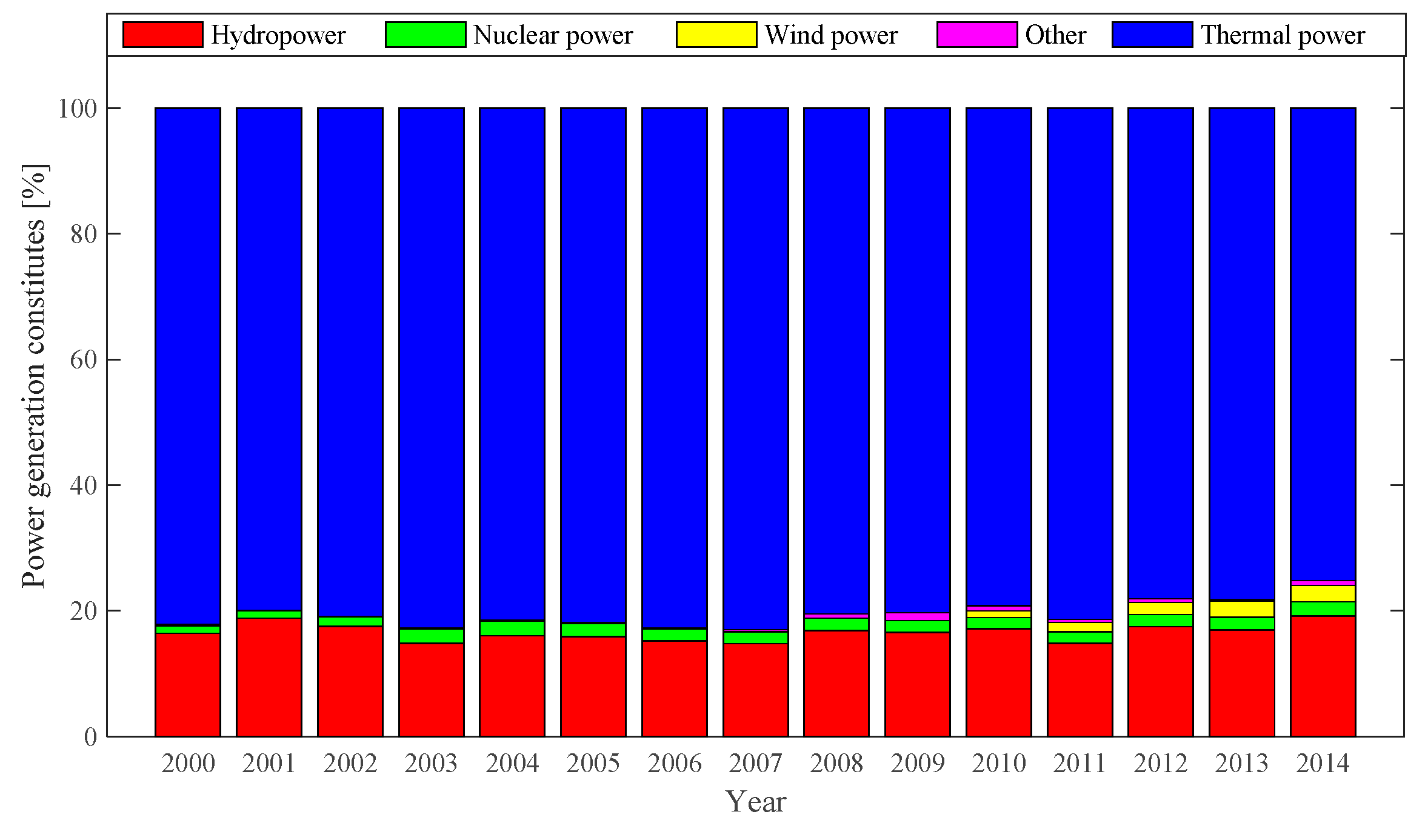
(4) A low-carbon economy causes a structural variation of electricity demand. Increasing electricity demand is mainly involved in renewable clean energy, like water power, nuclear power and wind power. With respect to a low-carbon scenario, i.e., unchanged energy efficiency, incremental 72.0263 million MW·h electricity demand is also chiefly centralized in renewable clean energy electricity demand compared with the baseline scenario. Despite the continuous effort on electricity structure adjustment and decreasing the ratio of coal power, the coal power ratio will not fall sharply for a time behind the reason of over-dependence on electricity and abundant coal resources. Illustrated in baseline scenario of Figure 13, power generation is presumed to be 70% coal power ratio and 30% in water power, nuclear power and wind power, which accounts for 238.5022 million MW·h in 2020. Due to the constrained energy policy, under the unchanged energy efficiency situation, electricity demand from clean energy approaches nearly 2601.1011 million MW·h by 2020, which accounts for 32.72% of total electricity demand, while the coal power ratio decreased to 67.28%. Therefore, the low-carbon economy has affected both electricity demand and its structure variation.

6. Conclusions

In this study, a new framework of combination forecasting electricity demand model is characterized as follows: (1) Integration of a grey relation degree with an induced ordered weighted harmonic averaging operator to propose a new weight determination method of combination forecasting model on basis of forecasting accuracy as induced variables; (2) utilization of the proposed weight determination method to construct the optimal combination forecasting model based on an extreme learning machine forecasting model and multiple regression model; (3) three scenarios in line with realization level of various low-carbon economy targets and dynamic simulation of the effects of a low-carbon economy on future electricity demand.
Resultant findings are obtained and clarified in detail: (1) the grey relation degree of reciprocal series between proposed combination forecasting value and actual values is better than the single forecasting models studied in this paper and corresponds to an optimal combination forecasting model; (2) the proposed combination forecasting model outperformed and concentrated the advantages of some monomial forecasting models, especially in boosting the overall instability dramatically and providing reliable decision basis; (3) the energetic progress of a low-carbon economy causes an increase in electricity demand and the relevant structure adjustment of electricity demand, especially in the increasing demand of clean energy. Above all, this study is aimed at providing a reference for future power planning issues in China.

Acknowledgments

This work is supported by the Natural Science Foundation of China (Project No. 71471059).

Author Contributions

Yi Liang designed this research and wrote this paper; Dongxiao Niu and Wei-Chiang Hong provided professional guidance; and Ye Cao collected all the data and translated this paper.

Conflicts of Interest

The authors declare no conflict of interest.

References

  1. Sevik, S. An analysis of the current and future use of natural gas-fired power plants in meeting electricity energy needs: The case of Turkey. Renew. Sustain. Rev. 2015, 52, 572–586. [Google Scholar] [CrossRef]
  2. O’Connell, N.; Pinson, P.; Madsen, H. Benefits and challenges of electrical demand response: A critical review. Renew. Sustain. Rev. 2014, 39, 686–699. [Google Scholar] [CrossRef]
  3. Fan, D.; Wang, S.; Zhang, W. Research on Prediction of China’s Electric Power Demand under Low-Carbon Economy Target. Power Syst. Technol. 2012, 36, 19–25. (In Chinese) [Google Scholar]
  4. Kang, C.; Chen, Q.; Xia, Q. Prospects of Low-Carbon Electricity. Power Syst. Technol. 2009, 33, 1–7. (In Chinese) [Google Scholar]
  5. Zeng, M.; Yang, Y.; Wang, L.; Sun, J. The power industry reform in China 2015: Policies, evaluations and solutions. Renew. Sustain. Energy Rev. 2016, 57, 94–110. [Google Scholar] [CrossRef]
  6. Yang, L.; Lin, B. Carbon dioxide-emission in China’s power industry: Evidence and policy implications. Renew. Sustain. Energy Rev. 2016, 60, 258–267. [Google Scholar] [CrossRef]
  7. Yun, L.; Ping, H. The Policy Interpretation of the Energy Conservation Power Generating and Distribution Code. J. Electr. Power 2008, 23, 215–217. (In Chinese) [Google Scholar]
  8. National Development and Reform Commission. The Twelfth Five Years Plan of Renewable Energy Development; National Development and Reform Commission: Beijing, China, 2013. (In Chinese)
  9. Zhang, C.; Yan, J. CDM’s influence on technology transfers: A study of the implemented clean development mechanism projects in China. Appl. Energy 2015, 158, 355–365. [Google Scholar] [CrossRef]
  10. D’Errico, M.C.; Bollino, C.A. Bayesian Analysis of Demand Elasticity in the Italian Electricity Market. Sustainability 2015, 7, 12127–12148. [Google Scholar] [CrossRef]
  11. Hernandez, L.; Baladron, C.; Aguiar, J.M. Classification and Clustering of Electricity Demand Patterns in Industrial Parks. Energies 2012, 5, 5215–5228. [Google Scholar] [CrossRef]
  12. Schweizer, V.J.; Morgan, M.G. Bounding US electricity demand in 2050. Technol. Forecast. Soc. Chang. 2016, 105, 215–223. [Google Scholar] [CrossRef]
  13. Trotter, I.M.; Bolkesjø, T.F.; Féres, J.G.; Hollanda, L. Climate Change and Electricity Demand in Brazil: A Stochastic Approach. Energy 2016, 102, 596–604. [Google Scholar] [CrossRef]
  14. Kishita, Y.; Yamaguchi, Y.; Umeda, Y. Describing Long-Term Electricity Demand Scenarios in the Telecommunications Industry: A Case Study of Japan. Sustainability 2016, 8, 52. [Google Scholar] [CrossRef]
  15. Seung, J.O.; Kim, C.N.; Kyaw, T.; Wongee, C.; Kian, J.E.C. Forecasting Long-term Electricity Demand for Cooling of Singapore’s Buildings Incorporating an Innovative Air-conditioning Technology. Energy Build. 2016, in press. [Google Scholar]
  16. Kandananond, K. Forecasting Electricity Demand in Thailand with an Artificial Neural Network Approach. Energies 2011, 4, 1246–1257. [Google Scholar] [CrossRef]
  17. Suhono, S. Long-term Electricity Demand Forecasting of Sumatera System Based on Electricity Consumption Intensity and Indonesia Population Projection 2010–2035. Energy Procedia 2015, 68, 455–462. [Google Scholar] [CrossRef]
  18. Pappas, S.S.; Ekonomou, L.; Moussas, V.C.; Karampelas, P.; Katsikas, S.K. Adaptive load forecasting of the Hellenic electric grid. J. Zhejiang Univ. Sci. A 2008, 9, 1724–1730. [Google Scholar] [CrossRef]
  19. Pappas, S.S.; Ekonomou, L.; Karamousantas, D.C.; Chatzarakis, G.E.; Katsikas, S.K.; Liatsis, P. Electricity demand loads modeling using autoregressive moving average (ARMA) models. Energy 2008, 33, 1353–1360. [Google Scholar] [CrossRef]
  20. Hussain, A.; Rahman, M.; Memon, J.A. Forecasting electricity consumption in Pakistan: The way forward. Energy Policy 2016, 90, 73–80. [Google Scholar] [CrossRef]
  21. Pérez-García, J.; Moral-Carcedo, J. Analysis and long term forecasting of electricity demand trough a decomposition model: A case study for Spain. Energy 2016, 97, 127–143. [Google Scholar] [CrossRef]
  22. Torrini, F.C.; Souza, R.C.; Cyrino-Oliveira, F.L. Long term electricity consumption forecast in Brazil: A fuzzy logic approach. Socio-Econ. Plan. Sci. 2016, 70, 101–114. [Google Scholar] [CrossRef]
  23. Zhao, H.R.; Zhao, H.R.; Guo, S. Using GM (1,1) Optimized by MFO with Rolling Mechanism to Forecast the Electricity Consumption of Inner Mongolia. Appl. Sci. 2016, 6, 20. [Google Scholar] [CrossRef]
  24. Fumo, N.; Biswas, M.A.R. Regression analysis for prediction of residential energy consumption. Renew. Sustain. Rev. 2015, 47, 332–343. [Google Scholar] [CrossRef]
  25. Günay, M.E. Forecasting annual gross electricity demand by artificial neural networks using predicted values of socio-economic indicators and climatic conditions: Case of Turkey. Energy Policy 2016, 90, 92–101. [Google Scholar] [CrossRef]
  26. Son, H.; Kim, C. Short-term forecasting of electricity demand for the residential sector using weather and social variables. Resour. Conserv. Recycl. 2016, in press. [Google Scholar] [CrossRef]
  27. Ekonomou, L.; Oikonomou, D.S. Application and comparison of several artificial neural networks for forecasting the Hellenic daily electricity demand load. In Proceedings of the 7th WSEAS International Conference on Artificial Intelligence, Knowledge Engineering and Data Bases (AIKED’08), Cambridge, UK, 20–22 February 2008; pp. 67–71.
  28. Huang, G.B.; Zhu, Q.Y.; Siew, C.K. Extreme learning machine: A new learning scheme of feedforward neural networks. In Proceedings of the 2004 IEEE International Joint Conference on Neural Networks, Budapest, Hungary, 25–29 July 2004; pp. 985–990.
  29. Bates, J.M.; Granger, C.W.J. Combination of forecasts. Oper. Res. Q. 1969, 20, 451–468. [Google Scholar] [CrossRef]
  30. Mao, L.; Yao, J.; Jin, Y.; Chen, H.; Li, W.; Guan, S. Theoretical Study of Combination Model for Medium and Long Term Load Forecasting. Proc. CSEE 2010, 30, 53–59. (In Chinese) [Google Scholar]
  31. Chen, H.; Sheng, Z. A Kind of New Combination Forecasting Method Based on Induced Ordered Weighted Geometric Averaging (IOWGA) Operator. J. Ind. Eng. Eng. Manag. 2005, 19, 36–39. (In Chinese) [Google Scholar]
  32. Zhao, W.; Wang, J.; Lu, H. Combining forecasts of electricity consumption in China with time-varying weights updated by a high-order Markov chain model. Omega 2014, 45, 80–91. [Google Scholar] [CrossRef]
  33. Chen, H. The Effectiveness Theory and Its Application of Combination Forecasting; Science Press Ltd.: Beijing, China, 2008. [Google Scholar]
  34. Chen, H.; Liu, C. A Kind of Combination Forecasting Method Baesd on Induced Ordered Weighted Averaging (IOWA) Operators. Forecasting 2003, 22, 61–65. (In Chinese) [Google Scholar]
  35. Chen, H.; Liu, C.; Sheng, Z. Induced Ordered Weighted Harmonic Averaging (IOWHA) Operator and Its Application to Combination Forecasting Method. Chin. J. Manag. Sci. 2004, 12, 35–40. (In Chinese) [Google Scholar]
  36. Chen, H.; Zhao, J.; Liu, C. Properties of combination forecasting model based on degree of grey incidence. J. Southeast Univ. (Natl. Sci. Ed.) 2004, 34, 130–134. (In Chinese) [Google Scholar]
  37. Hu, J. Firmly March on the Path of Socialism with Chinese Characteristics and Strive to Complete the Building of a Moderately Prosperous Society in All Respects. In Proceedings of the Report to the 18th National Congress of the Communist Party of China, Beijing, China, 8 November 2012.
  38. National Bureau of Statistics of the People’s Republic of China. China Statistical Yearbook 2015; China Statistics Press: Beijing, China, 2016. [Google Scholar]
  39. Xinhua News Agency. The Thirteenth Five-Year Plan for National Economic and Social Development of the People’s Republic of China; Xinhua News Agency: Beijing, China, 2016. [Google Scholar]
  40. Laicane, I.; Blumberga, D.; Blumberga, A.; Rosa, M. Comparative Multiple Regression Analysis of Household Electricity use in Latvia: Using Smart Meter Data to Examine the Effect of Different Household Characteristics. Energy Procedia 2015, 72, 49–56. [Google Scholar] [CrossRef]
  41. Xie, C.; Hawkes, A.D. Estimation of inter-fuel substitution possibilities in China’s transport industry using ridge regression. Energy 2015, 88, 260–267. [Google Scholar] [CrossRef]
Figure 1. Annual electricity consumption of China.
Energies 09 00941 g001
Figure 2. Scenario parameter setting.
Energies 09 00941 g002
Figure 3. GRD-IOWHA operator-based combination forecasting modeling process.
Energies 09 00941 g003
Figure 4. Ridge trace of variables.
Energies 09 00941 g004
Figure 5. Determination coefficient and K value.
Energies 09 00941 g005
Figure 6. Ridge trace of variables.
Energies 09 00941 g006
Figure 7. Determined coefficient and K value.
Energies 09 00941 g007
Figure 8. Forecasting accuracy comparison of single forecasting models in various scenario.
Energies 09 00941 g008
Figure 9. Electricity demand forecasting of various model in 2009–2014.
Energies 09 00941 g009
Figure 10. Relative error forecasting of various model in 2009–2014.
Energies 09 00941 g010
Figure 11. Evaluation index of various forecasting model.
Energies 09 00941 g011
Figure 12. Electricity demand forecasting trend of various model in 2015–2020.
Energies 09 00941 g012
Figure 13. Constitution and proportion of China’s annual power generation.
Energies 09 00941 g013
Table 1. Historical data of scenario parameter.
YearElectricity Demand (105 MW·h)GDP (1012 Yuan)Population (108 People)CO2 Emission Per GDP (104 Tons Standard Coal)Energy Consumption Per GDP (104 Tons Standard Coal)
200013,472.49.9812.670.971.49
200114,633.511.0312.760.921.43
200216,331.512.1012.850.911.42
200319,031.613.6612.920.951.45
200421,971.416.0713.000.941.44
200524,940.318.5913.080.931.42
200628,588.021.7713.140.861.32
200732,711.826.8013.210.761.16
200834,541.431.6813.280.651.01
200937,032.234.5613.350.630.97
201041,934.540.8913.410.560.89
201147,000.948.4113.470.520.81
201249,762.653.4113.540.480.75
201354,203.458.8013.610.450.71
201456,263.163.6113.680.420.67
Table 2. Scenario parameter setting.
YearGDP (1012 Yuan)Population (108 People)CO2 Emission Per GDP (104 Tons Standard Coal)Energy Consumption Per GDP (104 Tons Standard Coal)
201568.0613.750.400.65
201672.8313.820.390.63
201777.9213.880.370.61
201883.3813.950.360.59
201989.2214.020.340.57
202095.4614.090.330.55
Data source: NBS (National Bureau of Standards) and National Development and Reform Commission Energy Research Institute.
Table 3. Single test result in baseline scenario.
YearElectricity Demand (105 MW·h)RAELM
Value (105 MW·h)Forecasting AccuracyValue (105 MW·h)Forecasting Accuracy
200937,032.237,730.040.981236,680.390.9905
201041,934.541,728.510.995142,509.000.9863
201147,000.946,235.470.983747,442.710.9906
201249,762.649,881.220.997648,473.750.9741
201354,203.453,693.620.990653,276.520.9829
201456,263.157,258.170.982355,908.640.9937
Table 4. Single forecasting result in baseline scenario.
YearRA Forecasting (105 MW·h)ELM Forecasting (105 MW·h)
201560,670.0158,713.27
201664,215.0763,592.23
201767,687.0566,181.66
201871,527.1270,297.18
201975,530.3474,664.38
202079,708.1578,938.27
Table 5. Combination forecasting results in baseline scenario of 2015–2020.
YearGRD-IOWHA Forecasting (105 MW·h)
201560,133.92
201664,047.27
201767,277.69
201871,193.91
201975,296.73
202079,500.74
Table 6. Single test result in low-carbon scenario.
YearElectricity Demand (105 MW·h)RAELM
Value (105 MW·h)Forecasting AccuracyValue (105 MW·h)Forecasting Accuracy
200937,032.236,540.790.986737,683.970.9824
201041,934.540,878.390.974842,408.360.9887
201147,000.945,390.340.965747,461.510.9902
201249,762.649,709.480.998950,265.200.9899
201354,203.453,914.260.994755,531.380.9755
201456,263.158,759.430.955656,893.250.9888
Table 7. Single forecasting result in low-carbon scenario.
YearRA Forecasting (105 MW·h)ELM Forecasting (105 MW·h)
201562,954.4959,313.86
201667,435.3264,549.11
201771,839.9068,457.73
201876,984.7472,365.06
201982,518.0379,509.00
202088,473.9685,959.43
Table 8. Combination forecasting result in low-carbon scenario.
YearGRD-IOWHA Forecasting (105 MW·h)
201560,367.81
201665,394.08
201769,444.76
201873,700.24
201980,394.04
202086,703.37
Table 9. Single test result in reinforced low-carbon scenario.
YearElectricity Demand (105 MW·h)RAELM
Value (105 MW·h)Forecasting AccuracyValue (105 MW·h)Forecasting Accuracy
200937,032.236,565.660.987436,295.260.9801
201041,934.541,044.150.978842,639.000.9832
201147,000.945,822.550.974947,673.010.9857
201249,762.650,249.020.990250,270.180.9898
201354,203.454,581.740.993054,837.580.9883
201456,263.159,514.140.942257,697.810.9745
Table 10. Single forecasting result in reinforced low-carbon scenario.
YearRA forecasting (105 MW·h)ELM forecasting (105 MW·h)
201563,665.1164,261.28
201668,092.7368,235.02
201772,466.8173,265.20
201877,553.9377,386.74
201983,027.1582,835.97
202088,921.5588,110.93
Table 11. Combination forecasting result in low-carbon scenario.
YearGRD-IOWHA Forecasting (105 MW·h)
201564,048.9
201668,184.57
201772,980.49
201877,445.86
201982,903.57
202088,396.27
Table 12. Grey relation degree comparison in various scenarios.
Scene 1
ModelRAELMGRD-IOWHA
Grey correlation value0.66610.59450.9693
Scene 2
ModelRAELMGRD-IOWHA
Grey correlation value0.58040.60780.8532
Scene 3
ModelRAELMGRD-IOWHA
Grey correlation value0.71130.75030.9077
Table 13. Comparison of model forecasting result.
YearScene 1Scene 2Scene 3
IOWHATCFIOWHATCFIOWHATCF
200937,197.8137,268.1937,103.5837,386.7436,429.9736,297.96
201042,115.1442,071.9341,629.3242,010.5741,826.3842,623.05
201146,831.3146,766.6646,402.8346,923.0146,729.4747,654.51
201249,167.4149,261.9349,985.850,120.7150,259.650,269.97
201353,484.2653,510.154,710.8755,110.9354,709.3654,835.02
201456,575.3656,664.3857,811.2857,378.4658,591.957,715.97
Unit: 105 MW·h.

