
Control Optimization of Solar Thermally Driven Chillers


Abstract
:1. Introduction
2. Methodology
2.1. Control Approach
2.2. Investigated Control Strategies
2.2.1. Mode 1
2.2.2. Mode 2
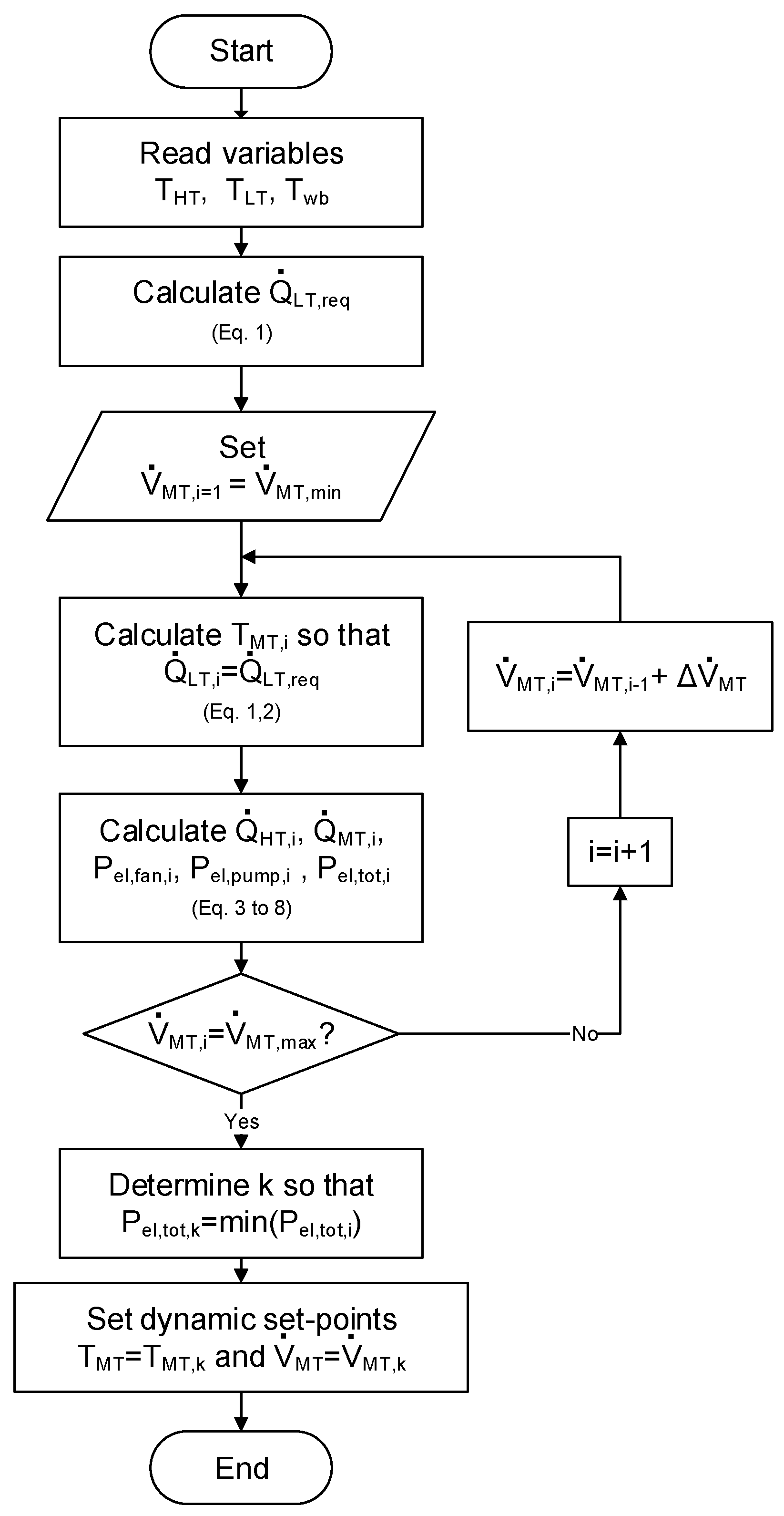
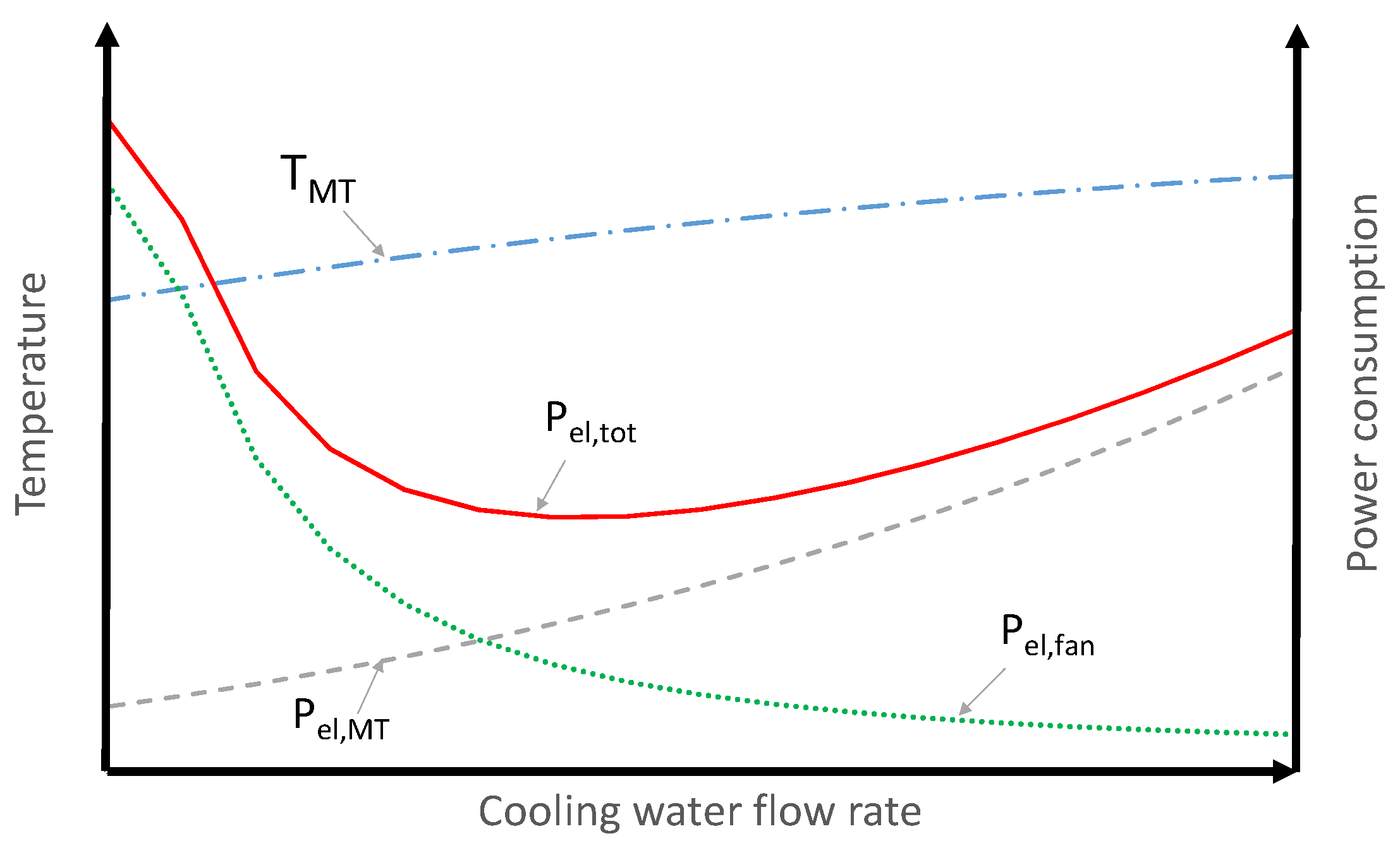
2.2.3. Mode 3
2.2.4. Overview
2.3. Performance Indicators
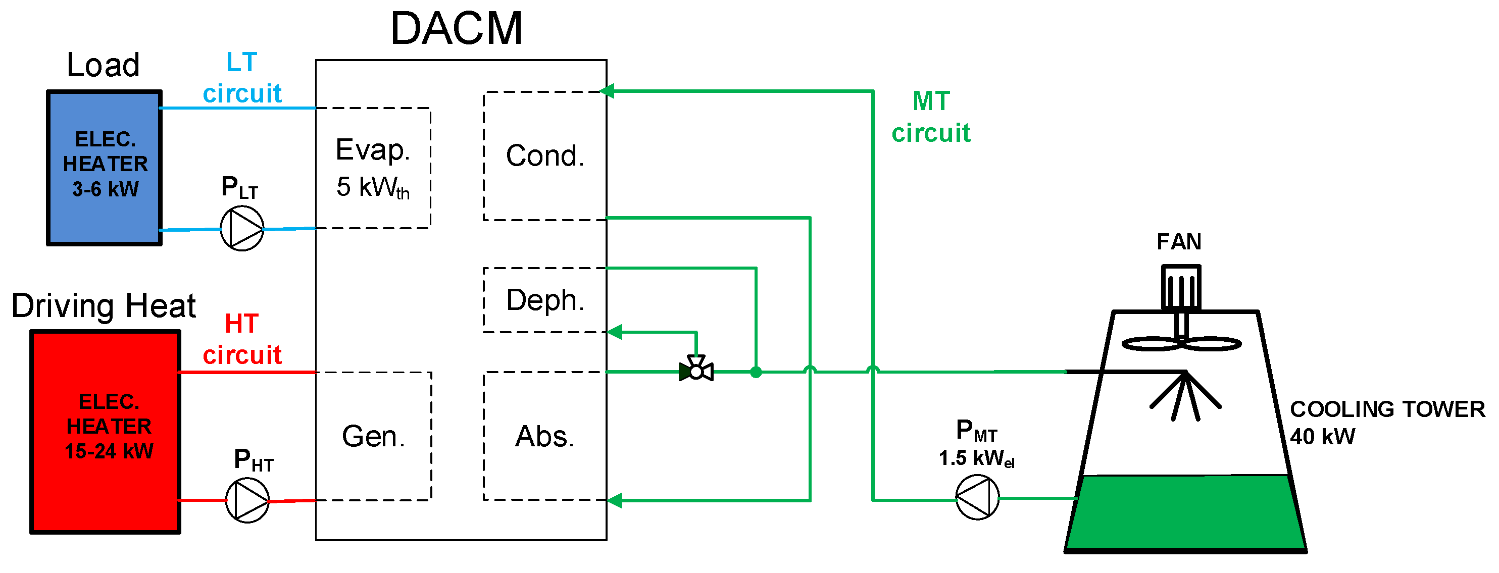
3. Experimental Set-Up
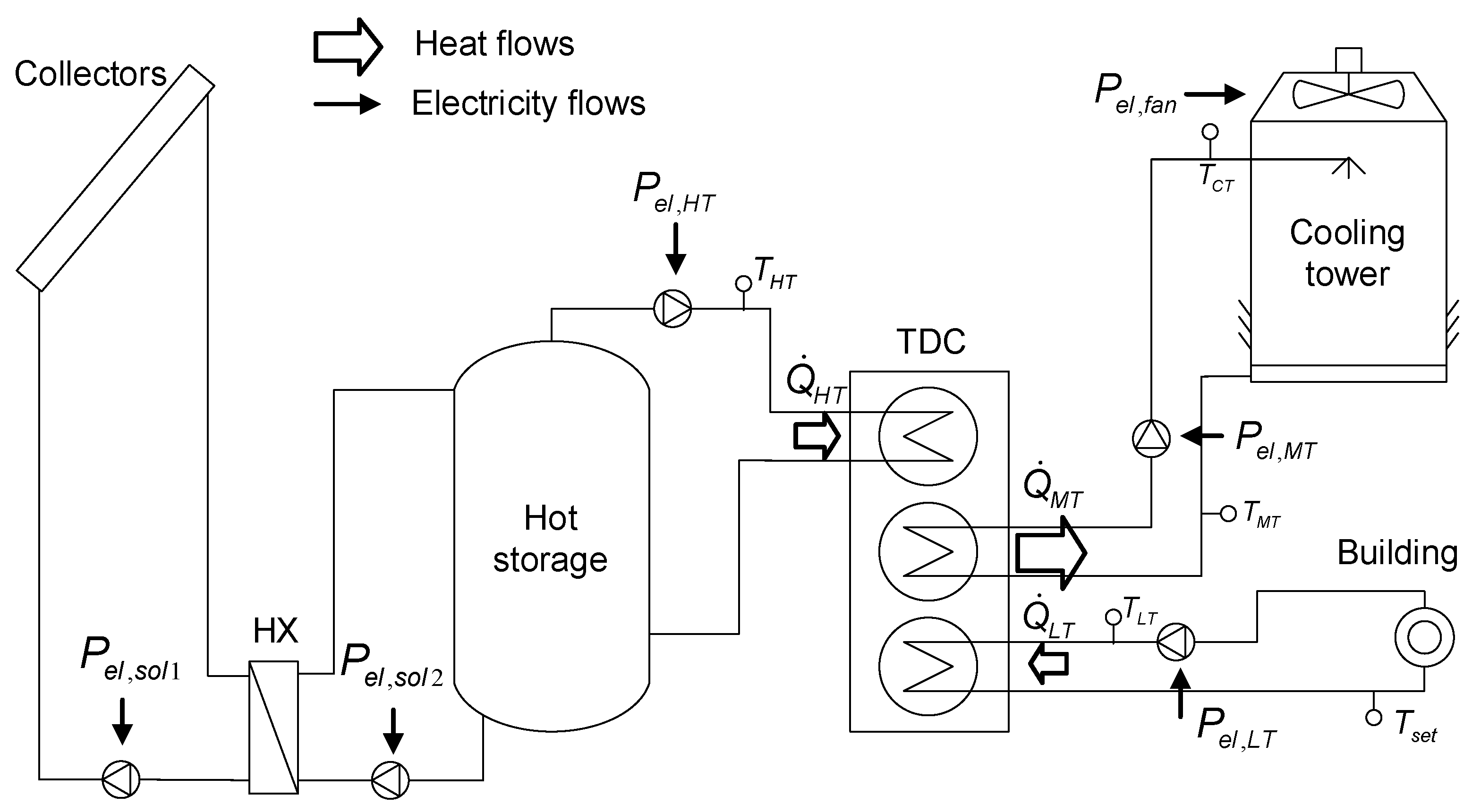
3.1. Description
3.1.1. Hardware Components
3.1.2. Measurement Devices
3.1.3. Data Acquisition and Control
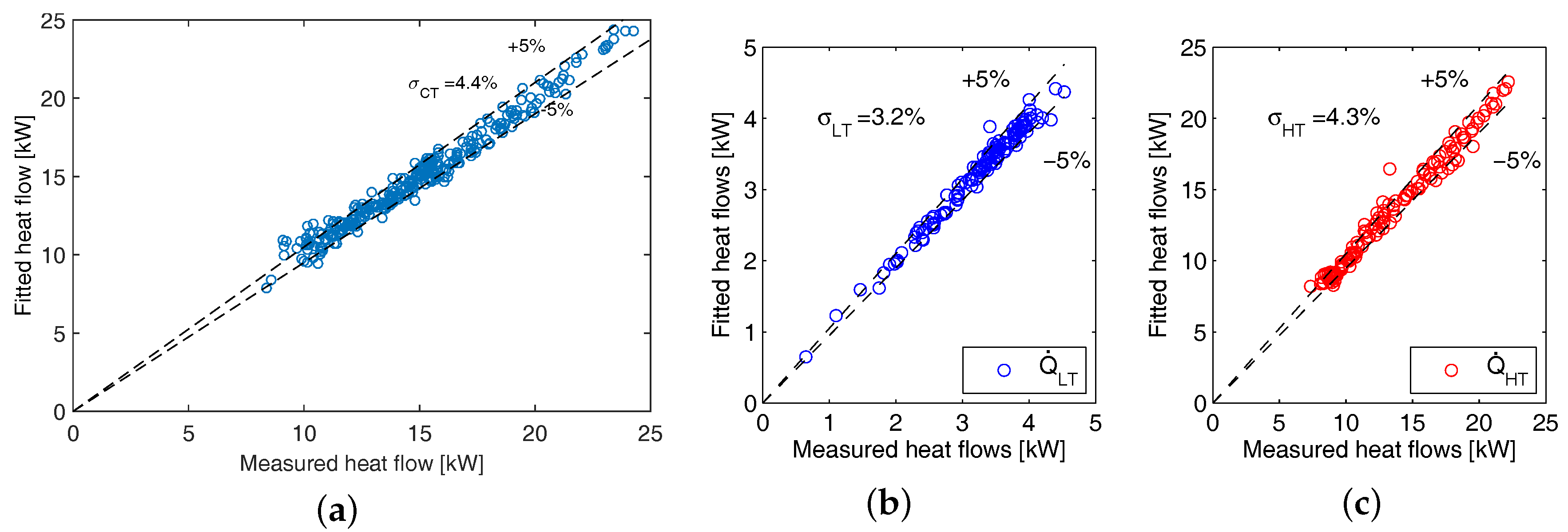
3.2. Characterization of the Main Components
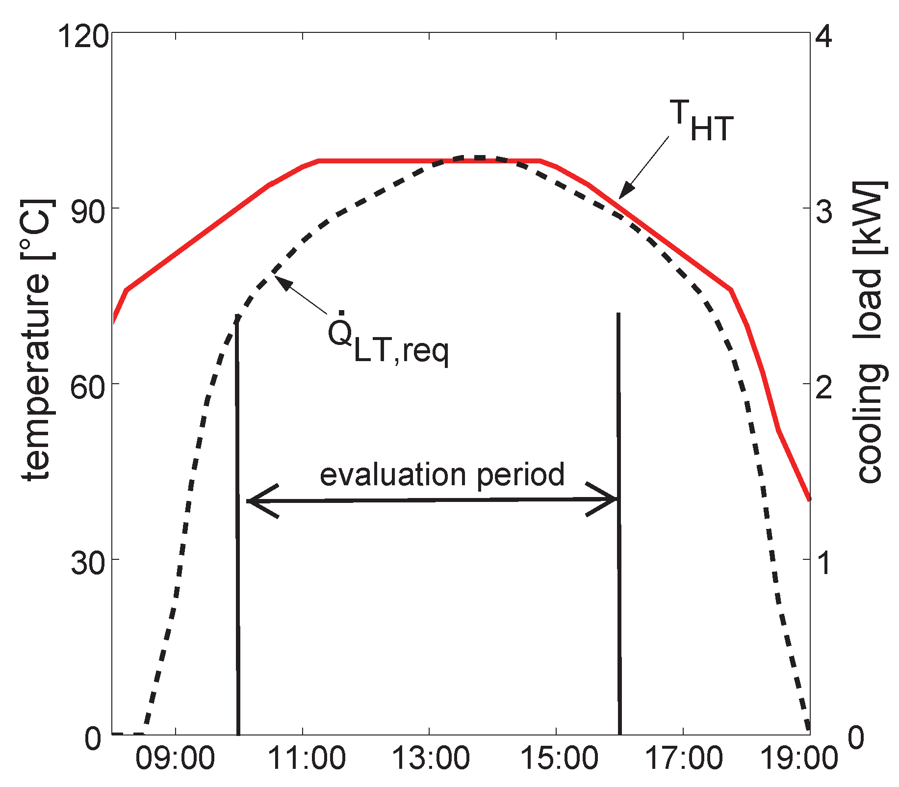
3.3. Investigated Daily Profile
4. Results
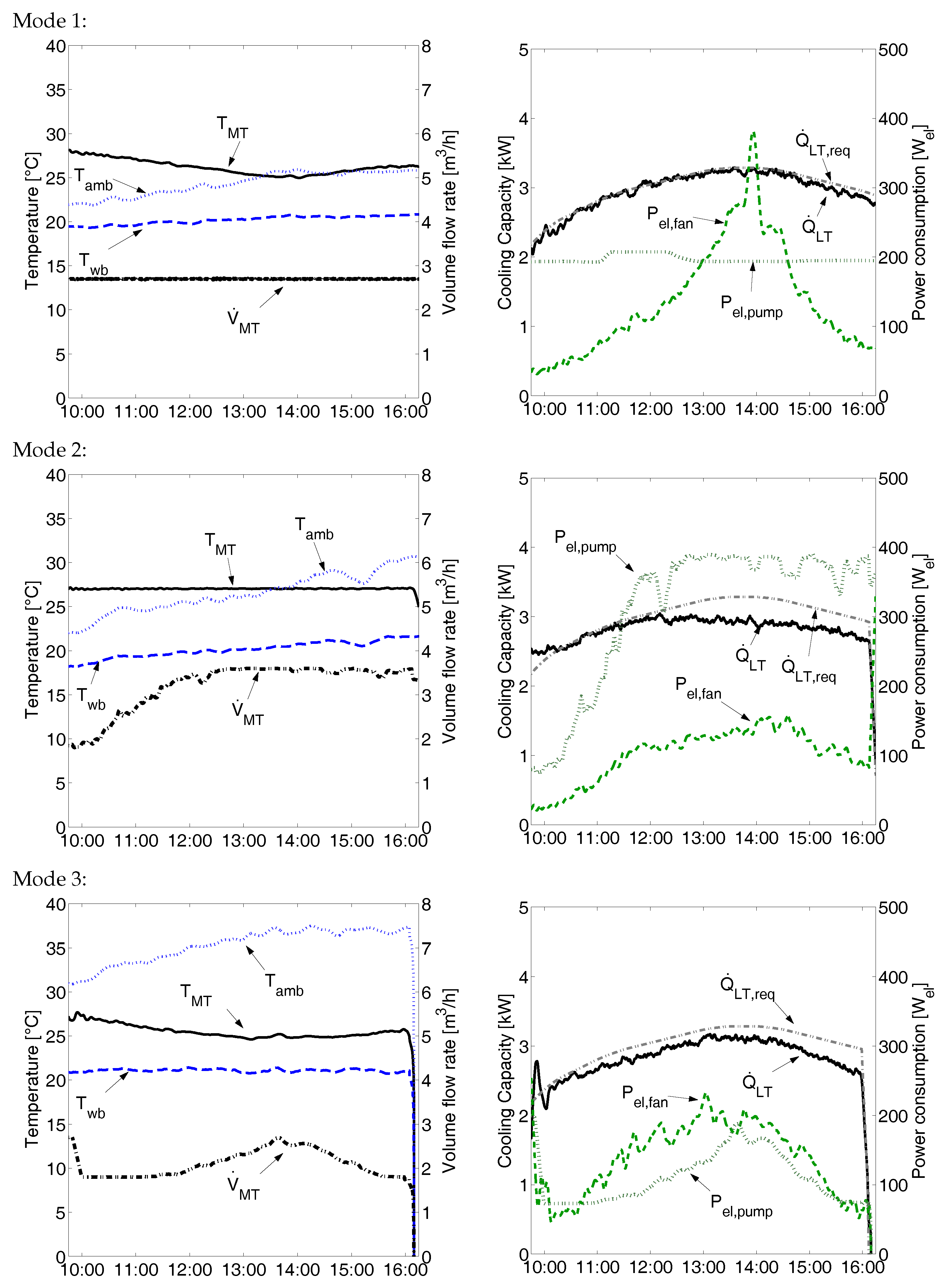
4.1. Experiments
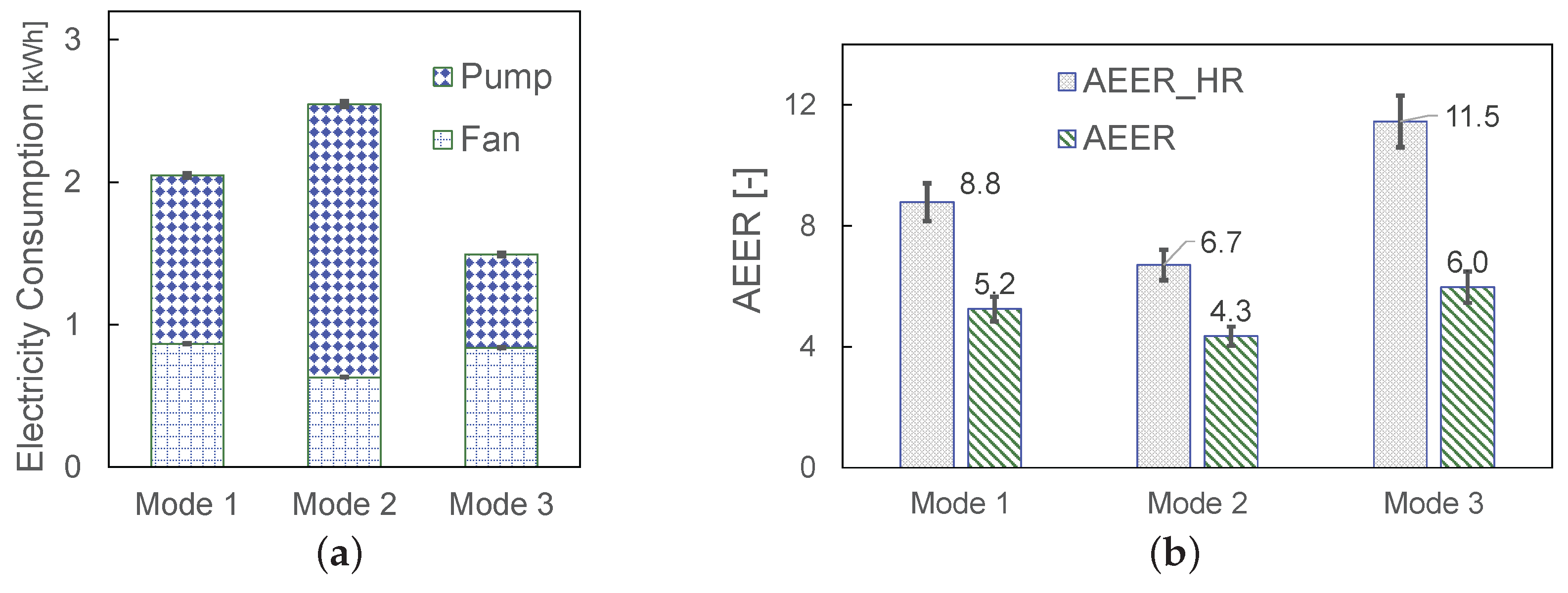
4.2. Performance Assessment
5. Conclusions
Acknowledgments
Author Contributions
Conflicts of Interest
Abbreviations
| Average energy efficiency ratio | |
| COP | Coefficient of performance |
| Chilled water mean specific heat () | |
| DACM | Diffusion absorption chilling machine |
| Energy efficiency ratio (-) | |
| Fan speed frequency (Hz) | |
| Pump speed frequency (Hz) | |
| HVAC | Heating ventilation and air conditioning |
| Power consumption of pump x (kW) | |
| Power consumption of cooling tower fan (kW) | |
| Total system power consumption (kW) | |
| Chiller desorber capacity (kW) | |
| Chiller heat rejection capacity (kW) | |
| Chiller cooling capacity (kW) | |
| STCS | Solar Thermally driven cooling systems |
| TDC | Thermally driven chiller |
| Dry bulb or ambient temperature (C) | |
| Wet bulb temperature (C) | |
| Hot water temperature (C) | |
| Cooling water temperature (C) | |
| Chilled water temperature (C) | |
| Chilled water temperature set point (C) | |
| Hot water flow rate () | |
| Cooling water flow rate () | |
| Chilled water flow rate () | |
| Temperature lift (C) | |
| Temperature thrust (C) | |
| Chilled water mean density () |
Appendix A
Appendix B
Appendix C

References
- Coulomb, D.; Dupon, J.L.; Pichard, A. The Role of Refrigeration in the Global Economy—29th Informatory Note on Refrigeration Technologies; Technical Report; International Institute of Refrigeration: Paris, France, 2015. [Google Scholar]
- Arent, D.J.; Tol, R.S.J.; Faust, E.; Hella, J.P.; Kumar, S.; Strzepek, K.M.; Toth, F.L.; Yan, D. Climate Change 2014: Impacts, Adaptation, and Vulnerability. Part A: Global and Sectoral Aspects. Contribution of Working Group II to the Fifth Assessment Report of the Intergovernmental Panel of Climate Change; Chapter Key Economic Sectors and Services; Cambridge University Press: Cambridge, UK; New York, NY, USA, 2014. [Google Scholar]
- European Commission. Commission Staff Working Document, Review of Available Information, Communication from the Commission to the European Parliament, the Council, the European Economic and Social Committee and the Committee of the Regions on an EU Strategy for Heating and Cooling; SWD (2016) 24 Final, PART 1/2; European Commission: Brussels, Belgium, 2016. [Google Scholar]
- European Commission. Communication from the Commission to the European Parliament, the Council, the European Economic and Social Committee and the Committee of the regions. A Policy Framework for Climate and Energy in the Period from 2020 to 2030; COM/2014/015 Final; European Commission: Brussels, Belgium, 2014. [Google Scholar]
- Henning, H.; Döll, J. Solar Systems for Heating and Cooling of Buildings—1st International Conference on Solar Heating and Cooling for Buildings and Industry (SHC 2012). Energy Procedia 2012, 30, 633–653. [Google Scholar] [CrossRef]
- Calise, F. Thermoeconomic analysis and optimization of high efficiency solar heating and cooling systems for different Italian school buildings and climates. Energy Build. 2010, 42, 992–1003. [Google Scholar] [CrossRef]
- Reda, F.; Viot, M.; Sipilä, K.; Helm, M. Energy assessment of solar cooling thermally driven system configurations for an office building in a Nordic country. Appl. Energy 2016, 166, 27–43. [Google Scholar] [CrossRef]
- Jähnig, D.; Thür, A. Monitoring Results—Technical Report of Substask A, Pre-Engineering Systems for Residential and Small Commercial Applications; IEA-SHC–Task38–Solar Air-Conditioning and Refrigeration; Solar Heating & Cooling Programme (SHC): Graz, Austria, 2011. [Google Scholar]
- Kohlenbach, P. Solar Cooling with Absorption Chillers: Control Strategies and Transient Chiller Performance. Ph.D. Thesis, TU Berlin, Berlin, Germany, 2006. [Google Scholar]
- Bujedo, L.; Rodríguez, J.; Martínez, P. Experimental results of different control strategies in a solar air-conditioning system at part load. Sol. Energy 2011, 85, 1302–1315. [Google Scholar] [CrossRef]
- Henning, H. Solar assisted air conditioning of buildings—An overview. Appl. Therm. Eng. 2007, 27, 1734–1749. [Google Scholar] [CrossRef]
- Lecuona, A.; Ventas, R.; Venegas, M.; Zacarías, A.; Salgado, R. Optimum hot water temperature for absorption solar cooling. Sol. Energy 2009, 83, 1806–1814. [Google Scholar] [CrossRef]
- Kühn, A.; Corrales Ciganda, J.; Ziegler, F. Comparison of control strategies of solar absorption chillers. In Proceedings of the 1st International Congress on Heating, Cooling and Buildings (EUROSUN 2008), Lisbon, Portugal, 7–10 October 2008.
- Ziegler, F.; Schweigler, C.; Hellmann, H. The characteristic equation of sorption chillers. In Proceedings of the International Sorption Heat Pump Conference, Munich, Germany, 24–26 March 1999; pp. 169–172.
- Sonntag, C.; Ding, H.; Engell, S. Supervisory Control of a Solar Air Conditioning Plant with Hybrid Dynamics. Eur. J. Control 2008, 14, 451–463. [Google Scholar] [CrossRef]
- Albers, J.; Kemmer, H.; Ziegler, F. Solar-driven adsorption chiller controlled by hot and cooling water temperature. In Proceedings of the 3rd International Conference Solar Air-Conditioning, Palermo, Italy, 30 September–2 October 2009.
- Albers, J. New absorption chiller and control strategy for the solar assisted cooling system at the German federal environment agency. Int. J. Refrig. 2014, 39, 48–56. [Google Scholar] [CrossRef]
- Dalibard, A.; Eicker, U.; Ziegler, F. Advanced controls of solar driven adsorption chillers. In Proceedings of the 5th International Conference Solar Air-Conditioning, Bad Krozingen, Germany, 25–27 September 2013.
- Eicker, U.; Pietruschka, D.; Pesch, R. Heat rejection and primary energy efficiency of solar driven absorption cooling systems. Int. J. Refrig. 2012, 35, 729–738. [Google Scholar] [CrossRef]
- Jakob, U.; Eicker, U.; Schneider, D.; Taki, A.; Cook, M. Simulation and experimental investigation into diffusion absorption cooling machines for air-conditioning applications. Appl. Therm. Eng. 2008, 28, 1138–1150. [Google Scholar] [CrossRef]
- Wiemken, E.; Nienborg, B.; Koch, L. Report on the methodology of the virtual case study—Solarcombiplus European Project. Fraunhofer ISE, 2009.


| Mode | Variable Set Point | Control Parameter | Objective(s) |
|---|---|---|---|
| 1 | Fan speed | Cover load | |
| 2 | Pump speed | Cover load | |
| 3 | & | Fan and pump speed | Cover load & Minimize |
| Measurement Device | Type | Accuracy |
|---|---|---|
| Flow meter | MID | 0.2% |
| Temperature sensors | PT100 (1/3 class B) | 0.1 + 0.0017·T |
| Humidity sensor | Capacitive | 2% (rel. humidity) |
| Ambient temperature sensor | PT100 | 0.2 K |
| Electricity meter | Electronic | 0.5% |
| Variable | DACM | Cooling Tower | Unit | Step |
|---|---|---|---|---|
| 90–115 | - | C | 5 K | |
| 20–28 | - | C | 3 K | |
| 18 | - | C | - | |
| 2.9 | - | - | ||
| 1.8–3.6 | 1.8–3.6 | 0.45 | ||
| 0.72 | - | - | ||
| - | 20–36 | C | 5 K | |
| - | 7–23.5 | C | 3 K | |
| - | 50–100 | Hz | - |
© 2016 by the authors; licensee MDPI, Basel, Switzerland. This article is an open access article distributed under the terms and conditions of the Creative Commons Attribution (CC-BY) license (http://creativecommons.org/licenses/by/4.0/).
Share and Cite
Dalibard, A.; Gürlich, D.; Schneider, D.; Eicker, U. Control Optimization of Solar Thermally Driven Chillers. Energies 2016, 9, 864. https://doi.org/10.3390/en9110864
Dalibard A, Gürlich D, Schneider D, Eicker U. Control Optimization of Solar Thermally Driven Chillers. Energies. 2016; 9(11):864. https://doi.org/10.3390/en9110864
Chicago/Turabian StyleDalibard, Antoine, Daniel Gürlich, Dietrich Schneider, and Ursula Eicker. 2016. "Control Optimization of Solar Thermally Driven Chillers" Energies 9, no. 11: 864. https://doi.org/10.3390/en9110864
APA StyleDalibard, A., Gürlich, D., Schneider, D., & Eicker, U. (2016). Control Optimization of Solar Thermally Driven Chillers. Energies, 9(11), 864. https://doi.org/10.3390/en9110864