Article

Error Assessment of Solar Irradiance Forecasts and AC Power from Energy Conversion Model in Grid-Connected Photovoltaic Systems

1
Energy Department, Politecnico di Torino, corso Duca degli Abruzzi 24, Torino 10129, Italy
2
Department of Engineering and Architecture, University of Trieste, Via Valerio 10, Trieste 34127, Italy
*
Author to whom correspondence should be addressed.
Energies 2016, 9(1), 8; https://doi.org/10.3390/en9010008
Submission received: 15 October 2015 / Revised: 6 December 2015 / Accepted: 11 December 2015 / Published: 24 December 2015

Abstract

:
Availability of effective estimation of the power profiles of photovoltaic systems is essential for studying how to increase the share of intermittent renewable sources in the electricity mix of many countries. For this purpose, weather forecasts, together with historical data of the meteorological quantities, provide fundamental information. The weak point of the forecasts depends on variable sky conditions, when the clouds successively cover and uncover the solar disc. This causes remarkable positive and negative variations in the irradiance pattern measured at the photovoltaic (PV) site location. This paper starts from 1 to 3 days-ahead solar irradiance forecasts available during one year, with a few points for each day. These forecasts are interpolated to obtain more irradiance estimations per day. The estimated irradiance data are used to classify the sky conditions into clear, variable or cloudy. The results are compared with the outcomes of the same classification carried out with the irradiance measured in meteorological stations at two real PV sites. The occurrence of irradiance spikes in “broken cloud” conditions is identified and discussed. From the measured irradiance, the Alternating Current (AC) power injected into the grid at two PV sites is estimated by using a PV energy conversion model. The AC power errors resulting from the PV model with respect to on-site AC power measurements are shown and discussed.

1. Introduction

Photovoltaic (PV) generation strongly depends on weather conditions, in particular on solar irradiance and temperature. As such, availability of accurate weather forecast data is very important for PV system planning and operation. For grid-connected PV systems, the power injected into the grid is concentrated during sunlight hours, in which typically the maximum peak load occurs.
In the power system, the task of the Transmission System Operator (TSO) is to ensure a constant balance between supply and consumption within the grid. Actually, the presence of strong fluctuations of the irradiance increases the uncertainty on the PV generation and requires additional regulatory actions for the procurement of reserve services. This may cause an increase in the costs for ancillary services. The irradiance forecast is then useful for grid management, to obtain more accurate information on the expected weather conditions. This information may assist the operators in undertaking decisions concerning the energy market and to reduce the costs of energy imbalance.
The first research on solar irradiance forecasting was conducted more than twenty years ago [1], using the Model Output Statistics (MOS) technique [2]. This technique allows the prediction of a daily average value one or two days ahead. Concerning the forecasting on a short-time scale (a few hours), the effectiveness of a statistical approach based on the prediction of the motion of the clouds through images provided by satellites of the Meteosat constellation has been demonstrated in [3]. However, this method requires a huge computational effort. A multi-resolution decomposition technique applied to satellite images has been studied in [4], in order to obtain information on the local mean value and on the gradient of solar irradiance at different spatial scales. Other studies on short and very short time scales are available in the literature, taking into account the information provided by satellites. Currently, the weather forecasting tools are based on numerical techniques, which provide good results when applied to extended spatial scales. However, these tools are not able to address local variability of the weather conditions.
The forecasting field is rapidly evolving according to the growth of the PV market. A model to predict the power P produced by a PV plant can be written in the general form P = f ( X 1 , X 2 , ... , X n ) where Xi (i = 1, 2,…, n) are n different physical quantities of influence. These quantities, including the solar irradiance, the PV module’s temperature, the air temperature, the wind speed, the relative humidity, etc., have to be provided by forecasting tools. The input of many models is the solar irradiance [5], while different methods are based on the irradiance and on the temperature of the air or of the PV module [6]. In general, as shown in [7] the models based on irradiance and temperature perform better than the ones where only the irradiance is considered. Conversely, the adoption of the models based on other working conditions does not necessarily improve the prediction accuracy.
Different techniques showing accurate results have been used to predict the power produced by a PV plant. Some examples are Artificial Neural Networks (ANN)-based techniques [7,8,9], regression model-based techniques [10], support vector machine [11], hybrid models [12] and PV system models [13]. The prediction methods may change depending on the availability of local data coming from a weather station specifically designed and installed to measure the operating conditions of the PV system under study. Most residential PV plants (as well as many of the commercial/industrial ones) are not equipped with any sensor of climate conditions. In this case, the usage of commercial weather data allows the implementation of simpler models for the estimation of the power produced by the PV plants [14].
Recently, a growing interest in using spatio-temporal forecasting methods has emerged, due to the availability of time series data over a large number of meteorological stations. Interesting results incorporating spatial-temporal forecasting method based on the vector autoregression framework have been presented in [15]. This framework combines observations collected by smart meters and distribution transformer controllers, to obtain 6 h-ahead forecasts at the residential PV and medium-voltage/low-voltage substation levels. Spatio-temporal information from satellite images has been used in [16] through an autoregressive approach to forecast the global horizontal irradiance at ground level.
This paper presents a procedure to assess the errors occurring in the 1 day-ahead solar irradiance estimation and in the model-based estimation of the Alternating Current (AC) power delivered to the grid by the PV system. This procedure is based on:
(1)
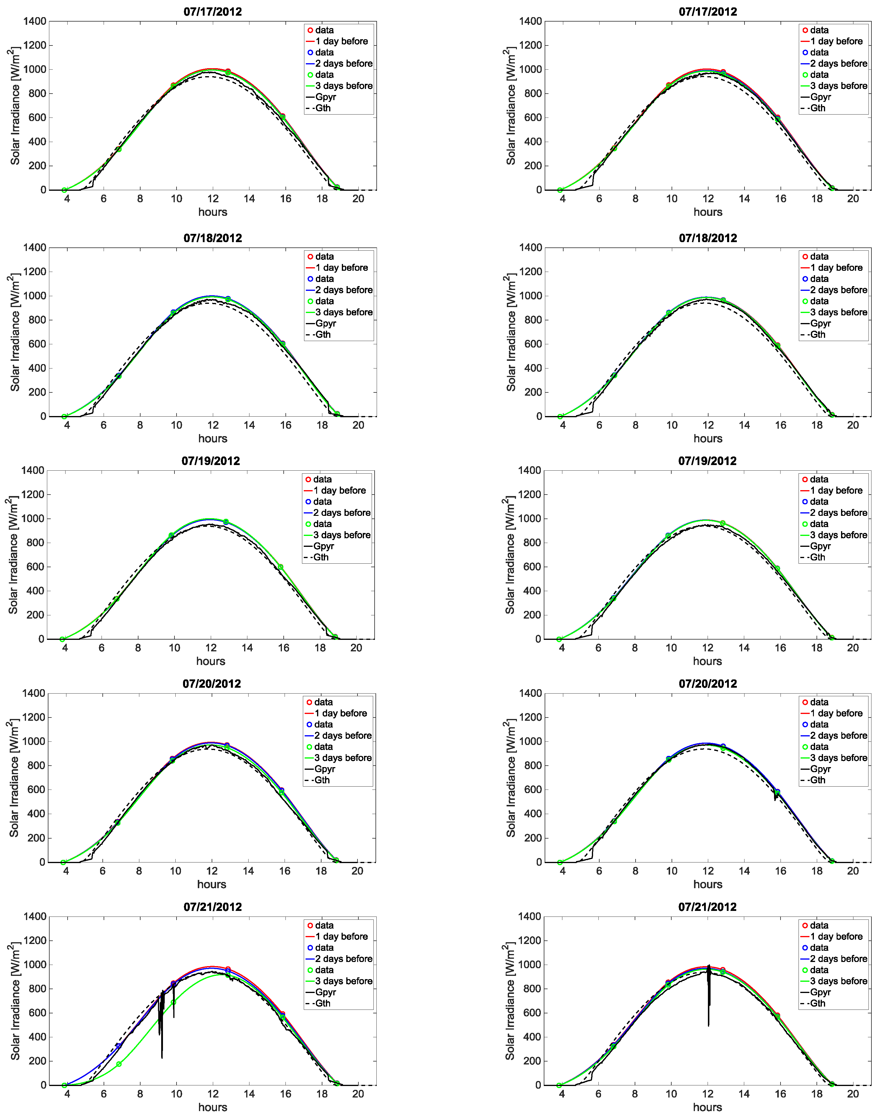
The use of solar irradiance weather forecasts updated every a few hours from a provider. These data are interpolated with polynomial splines to obtain a higher number of estimated values during the day. The results are compared with the measurements gathered at 1-min intervals during a period of one year in order to calculate the estimation error.
(2)
The application of a PV conversion model from solar irradiance to AC power, determining 1-min AC power estimates. From these values, 15-min averaged data are calculated and compared with the energy meter readings at 15-min intervals in order to calculate the error on AC power estimates.
The strengths of this paper are that:
(a)
The procedure presented can be used to select the best forecasting model or the best provider of weather forecasts in the location of interest.
(b)
The irradiance error estimation is particularly accurate, because the meteorological stations are equipped with pyranometers (secondary standards used as reference instruments) installed in the same sites of two operating PV plants. Moreover, the AC power error estimation is relevant because (i) the PV plants analyzed are located in the Italian region (Puglia) with the highest PV power density; and (ii) the measurements referring to the PV plants are taken from calibrated energy meters.
The results of the proposed procedure are presented in the form of duration curves of the positive and negative errors between estimated and measured values, determined during a period of one year. The evaluation of the estimation errors is helpful for the grid operator to estimate to what extent the estimation of the PV contribution as grid-connected local generation, calculated starting from 1 day-ahead forecast data, can be trustable. The occurrence of irradiance spikes due to the phenomenon of “broken clouds” is also presented and discussed as a source of possible irradiance peaks, in some cases exceeding the rated value of the AC power injected into the grid.
The next sections of this paper are organized as follows: the second section presents an overview of solar irradiance models and the PV conversion model. The third section introduces the proposed model for hourly classification in clear, variable and cloudy sky conditions, according to the clearness index values. Section 4 discusses the error calculation of the estimated irradiance with respect to the measured irradiance. The fifth section addresses the errors between the AC power estimates and the AC power values measured on two PV systems in operation. The last section contains the conclusions.

2. Solar Irradiance Models and PV System Description

2.1. Models for Extraterrestrial and Ground Level Irradiance

Solar irradiance, which is received by the Earth’s surface, is the result of complex interactions between the irradiance from the Sun, the atmosphere and the Earth’s surface. In general terms, it is subject to changes determined by the geometry of the Earth, its daily rotation and its annual revolution around the Sun. On a local scale, the main factor is the topography, especially the altitude, the slope, the exposure, and the shading caused by mountains or other natural obstacles. It is possible to determine, by means of appropriate geometric relationships, the amount of irradiance that reaches locally a plane parallel to the ground [17]. The first step is to determine the position of the Sun relative to an observer on the ground, by using a suitable reference system represented by the celestial coordinates. In this case, it is convenient to make use of local coordinates:
  • latitude ξ, in radians or degrees, with respect to the equator (>0 toward North);
  • longitude ζ, in radians or degrees, referred to the Greenwich line (>0 toward East);
  • solar declination δ, the angle between the Sun-Earth line and the equator plane (>0 North);
  • hour angle ψ, between the meridian plane passing through the observer and the meridian plane passing through the Sun (>0 West);
  • azimuth angle ϕ between the projection of the Sun-Earth line and the plane at the horizon with South direction (>0 West);
  • zenith angle z between the Sun-Earth line and the zenith direction;
  • solar height α, that is, the angle between the Sun-Earth line and the horizon plane.
The latitude ξ and the longitude ζ are the only parameters that do not require calculations, because they are known as the geographical coordinates of the place of observation.
The hour angle ψ of the Sun is a more complex parameter, because it depends on the position of the observer (longitude effect) and on the measurement of the local time. During the year, the time indicated from a meridian deviates periodically a few minutes with respect to the time indicated by a clock, which in Italy is normally referred to the Central European Time (CET). This difference is called “equation of time” τ, defined as the East or West component of the analemma, a curve representing the angular offset of the Sun from its mean position on the celestial sphere as viewed from the Earth. At any point in time, the solar irradiance incident on a horizontal plane outside the atmosphere is the normal solar irradiance G0, given by ([18], pp. 37–41):
G 0 = G s c ( 1 + 0.033 cos 360 d 365 ) cos z
where Gsc is the solar constant, d is the day of the year, and cos z = cos ξ cos δ cos ψ + sin ξ sin δ .
By integrating this equation for an interval between the hour angles ψ1 and ψ2, which define an hour (where ψ2 is the larger), the irradiation H0 (in MJ/m2) is obtained as:
H 0 = 12 × 3600 π G s c ( 1 + 0.033 cos 360 d 365 ) [ cos ξ cos δ ( sin ψ 2 sin ψ 1 ) + ( ψ 2 ψ 1 )   sin ξ sin δ ]
The solar irradiance, in the path through the atmosphere towards the Earth surface, is subject to scatter, absorption, reflection, diffusion, meteorological conditions and air mass [19]. It is useful to define a standard “clear” sky and calculate the hourly and daily irradiance that would be received on a horizontal surface under these standard conditions ([18], pp. 85–95). In order to calculate the clear sky irradiance, several methods have been developed [20]. Among these methods, the Moon-Spencer model [21] provides the theoretical instantaneous values of the irradiance at clear sky on a surface orientated in any direction. The irradiance values obtained from the Moon-Spencer model refer to free view with respect to the horizon. The results may differ in case of obstacles hiding the visual landscape, for some parts of the day, in the directions in which the Sun should impact on the surface (e.g., presence of mountains or adjacent buildings). In these cases, the results of the Moon-Spencer model have to be adjusted to take into account the actual skyline seen from the surface.
The Moon-Spencer model was developed for the atmospheric conditions in the United States, but sometimes it over-estimates or under-estimates the global irradiance in case of geographical locations different from the United States. Therefore, this clear sky model cannot be considered as an ideal profile with minimum turbidity of the sky, but it represents an indicative daily evolution for the comparison with the weather forecasts. In order to take into account the information provided by the clear-sky model, a dedicated variable space has been created in [22], in which the time axis is normalized in such a way to map the time interval between the sunrise and the sunset in the (0, 1) interval; the irradiance values are normalized so that the unity value corresponds to the peak conditions at clear-sky from the Moon-Spencer model.
Another clear-sky model has been implemented in the online software PVGIS [23]. In [24] a comparison between the irradiance measured by the pyranometer and the simulated PVGIS clear-sky irradiance has been discussed for a particular day of July. Examining other days during the whole year, owing to higher air turbidity the measured values are, many times, lower than the ones obtained from the clear-sky model.
In this paper, the data are elaborated in order to create a partitioning into three types of sky conditions: variable, clear, and cloudy. Classifications with more types of sky conditions have been used in various references for different purposes [25,26].

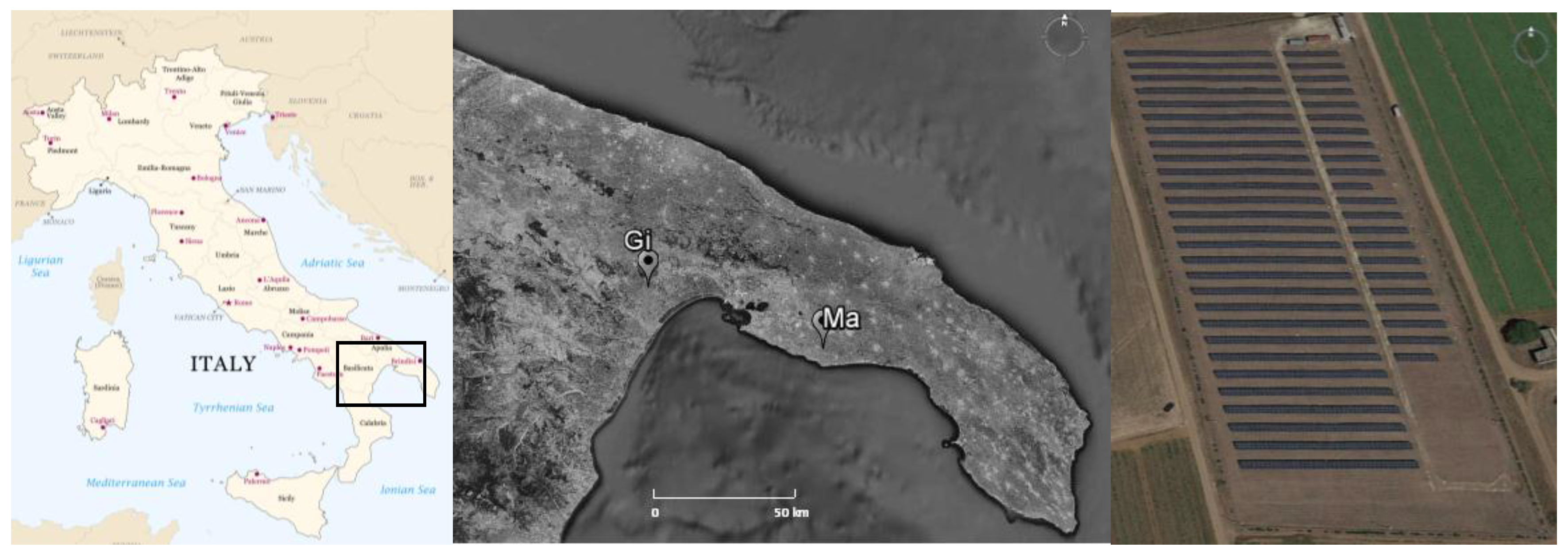
2.2. Description of the Two Meteorological Stations and PV Systems

For our investigation, measurements have been collected by two meteorological stations, named for the sake of simplicity “Gi” and “Ma”, near two grid-connected PV systems at latitude 40° North (Puglia region, Figure 1). The distance between the two meteorological stations is 61 km. As discussed in [27], each meteorological station is provided with:
  • A pyranometer (Secondary Standard according to ISO 9060 [28]) for measuring the horizontal global irradiance Gpyr;
  • Two reference solar cells in polycrystalline silicon (p-Si) with South orientation for measuring the 30° tilted global irradiance Gtcell;
  • One thermo-hygrometer for measuring the ambient temperature Tamb, relative humidity and wind speed ws.
Figure 1. Location of the two grid-connected PV systems and satellite photo of the “Gi” site.
Energies 09 00008 g001
To obtain a correctly integrated value for the solar irradiance over the day, small time steps are recommended for data sampling. However, due to the response time of the pyranometer, the time step cannot be lower than 5 s. The sampling time steps may be chosen depending on the data collection system and on the calculation and update speed of the algorithms used. In our case, the pyranometer is connected to the meteorological station. Therefore, a time step of 10 s and an averaging time for the integrated values of 1 min are used. This averaging time is suitable for obtaining a sufficient number of data to be further averaged within longer time steps, such as the ones used in the electricity markets (e.g., 10, 15 min, 30 min, or 1 h). The global irradiance data from solar cells on the tilted plane are validated through the comparison with the pyranometer uncertainty [24], showing the possible effect of the measurement accuracy. The expanded uncertainty of a pyranometer having the same characteristics of the pyranometers used in the two sites is about 30 W/m2 with confidence level 95% (coverage factor k = 2) [29]. This value is valid when the irradiance reaches its peaks up to 1200 W/m2. A confidence level 99.7% (coverage factor k = 3) corresponds to an expanded uncertainty of about 45 W/m2. At mid-level of irradiance (e.g., around 500 W/m2) the expanded uncertainty for k = 2 is about 15 W/m2.
The real grid-connected PV system has a power rating Ppeak = 993.6 kWp for the site “Gi” and Ppeak = 997.3 kWp for the site “Ma” at Standard Test Conditions (STC) with global irradiance GSTC = 1 kW/m2, cell temperature TSTC = 25 °C and standard spectrum AM 1.5. The PV system in the site “Gi” is equipped with polycrystalline silicon modules of 230 Wp each, tilted at 30° with South orientation. On the contrary, the PV system in the site “Ma” is equipped with mono-crystalline silicon modules of 230 Wp, 235 Wp and 240 Wp and with polycrystalline silicon modules of 230 Wp, 235 Wp and 240 Wp, tilted at 30° with South orientation. The PV arrays of each site, placed on a metallic structure that permits the natural air circulation, feed two centralized inverters with high efficiency (transformerless option). These power conditioning units are slightly undersized, given that the 500-kVA inverter is supplied by a 552.0 kWp array for the site “Gi” and by a 542.0 kWp array for the site “Ma”; the 400-kVA inverter is supplied by a 441.6 kWp array for the site “Gi” and by a 455.3 kWp array for the site “Ma”.

2.3. Definition of the PV Conversion Model

In the definition of the PV conversion model, it is important to take into account the efficiencies referring to the main loss factors affecting the PV system behavior. As mentioned in [30], the main loss factors are summarized in the efficiencies defined as follows:
  • Efficiency ηdirt, due to losses for soiling and dirt (environmental pollution). To estimate the impact of dirt/soiling accumulation, a 10-day summer period without rain is considered. At the end of this period (10th day), the horizontal solar irradiation is calculated from the pyranometer and the solar cell. At the 11th day, the rain appears and naturally cleans the sensors. Finally, at the 12th day (clear-sky day), the solar irradiation is calculated in such a way as to practically have the same astronomical conditions of the 10th day. Therefore, the corresponding value of ηdirt for the PV plant, located in a relatively clean environment (i.e., away from mines, landfills, etc.), is determined according to the following formula:
    η d i r t = 100 ( H a _ r a i n H b _ r a i n ) H a _ r a i n
    where Ha_rain and Hb_rain are the values of the daily irradiation in two clear-sky days, one after rain (12th day) and the other before rain (10th day), respectively. The corresponding value of ηdirt is generally in the range 0.97–0.98.
  • Efficiency ηrefl, due to reflection of the PV module glass; the value used is 0.971, taken from the PVGIS website [23].
  • Efficiency ηth, due to the thermal losses lth with respect to the STC, calculated as:
    η t h = 1 l t h = 1 γ t h ( T C T S T C )
    where γ t h is the thermal coefficient of maximum power of the PV modules, depending on the PV technology (for crystalline silicon γ t h = 0.5%/°C); TC is the cell temperature (mean temperature in outdoor operation at GNOCT = 800 W/m2 and Tamb,NOCT = 20 °C), which can be calculated as a function of the ambient temperature Tamb, the cell irradiance on the tilted plane Gtcell and the Normal Operating Cell Temperature (NOCT) of 42–50 °C [31,32]:
    T C = T a m b + ( N O C T T a m b , N O C T ) G t c e l l G N O C T
  • Efficiency ηmism, taking into account the current-voltage (I-V) mismatch losses, assuming that the bottleneck effect globally leads to 97% of the power rating declared by the manufacturer for all the modules in the PV array. This loss is a consequence of the weakest modules in the series connection inside the strings, and of the weakest strings in the parallel connection inside the PV array [33].
  • Efficiency ηcable, including the DC cable losses, with the value 0.99 considered according to good design criteria [34].
    Considering these efficiencies, the available power at the maximum power point is expressed as:
    P m p p = P r a t e d ( G t c e l l G lim ) η d i r t η r e f l η t h η m i s m η c a b l e
    where Glim = 17.7 W/m2 is the irradiance limit below which the output is vanishing, calculated by linear interpolation of the irradiance and power values declared by the manufacturer of the silicon modules installed in the PV array.
Finally, considering the efficiency ηMPPT of the maximum power point tracker, and thanks to the model of the power conditioning unit for grid connection, the AC power injected into the grid is calculated by solving the second-order equation [35]:
c Q P A C 2 + ( 1 + c L ) P A C + P 0 P D C = 0
with:
P D C = η M P P T P m p p
where P0 is the no-load power losses along the operation, while cL and cQ are the linear and quadratic loss coefficients, respectively.
Therefore, if the reference-cell data Gtcell, averaged on 15-min basis, are used as inputs of the above-described model, the power PAC delivered to the grid can be compared with the power Pmeas indicated by the energy meter of the PV plant.
For the error calculation of the AC power profiles compared to the experimental results of each PV plant in the two sites, the estimation error ΔP is defined as the difference between the estimated power to be delivered to the grid PAC and the AC power Pmeas measured by the energy meter of each PV plant:
Δ P = P A C P m e a s

3. Clear, Variable and Cloudy Sky Classification

3.1. Determination of the Diffuse Contribution in the Global Irradiance

The amount of solar irradiance that reaches the ground, besides the daily and yearly apparent motion of the Sun, depends on the geographical location (latitude and longitude) and on the climatic conditions (e.g., cloud coverage). Many studies have proved that cloudiness is the main factor affecting the difference between the values of irradiance measured outside the atmosphere and on the Earth surface [36].
Let us define the global irradiance on a horizontal surface Gth (kW/m2), composed of the diffuse component Gdh and beam component Gbh. Let us further consider the hourly clearness index kt = Gth/G0, calculated as the ratio of Gth (measured by the pyranometer) to the extra-atmospheric total irradiance G0 (kW/m2) defined in Equation (1). The ratio kd = Gdh/Gth can be expressed as a function of the clearness index, and permits to distinguish the sky conditions into clear, variable and cloudy. For this purpose, several correlations have been proposed to establish a relationship between the diffuse and the global horizontal irradiances. As explained in [37], some of the existing models [38,39] have been developed for Northern latitudes with high albedos and air masses. This is the reason for differences in diffuse irradiance values and an error source in modeling diffuse irradiance [40]. Only in recent years models to calculate the diffuse irradiance with respect to the global irradiance have been developed for the European Mediterranean area [41]. The hourly correlations considered in this context are represented by these expressions:
k d = { 0.995 0.081 k t for k t 0.21 0.724 + 2.738 k t 8.32 k t 2 + 4.967 k t 3 for 0.21 < k t 0.76 0.180 for k t > 0.76
The above-mentioned correlations permit the hourly classification of the sky conditions. In particular:
  • for kt ≤ 0.21 a total cloudy sky condition occurs, and a linear expression of kd is assumed;
  • in the range 0.21 < kt ≤ 0.76, a variable (i.e., partially cloudy) sky condition occurs, in which the Sun is partially obscured by clouds, and the correlation is represented by a cubic polynomial expression;
  • for kt > 0.76 a clear-sky condition occurs, in which that the sunlight is not reduced by clouds, and the fraction of diffuse irradiance is assumed to be 18% of the global one.
The weather forecasts considered in this paper are provided by the meteorological service of Catalonia [42]. The available data are based on the Weather Research and Forecasting (WRF) [43] model: a next-generation mesoscale numerical weather forecast system designed to serve both atmospheric research and operational forecasting needs. It features two dynamical cores, a data assimilation system, and a software architecture allowing for parallel computation and system extensibility. The model serves a wide range of meteorological applications across scales ranging from meters to thousands of kilometers. As shown in Table 1, the coordinates of the points of the WRF model (WRF latitude and WRF longitude) are close to the real points (real latitude and real longitude) for the two sites under analysis.
Table 1. Real and WRF coordinates for the two sites (degrees).
SiteReal LatitudeReal LongitudeWRF LatitudeWRF Longitude
Ma40.3517.5240.4417.65
Gi40.5516.8440.6216.93
The data set taken from the meteorological provider consists of solar irradiance forecasts for the two meteorological stations during the whole year 2012 [44]. The forecast values are given in W/m2 at four points in time (hours 7 a.m., 10 a.m., 1 p.m. and 4 p.m.). There is no indication on the uncertainty of these data. The maximum timespan is 72 h. The forecast data have been first interpolated by using polynomial splines [45], obtaining an estimated irradiance pattern that can be represented with a number of points per day higher than the four points available from the forecast data.
On the basis of the hourly correlations from Equation (10), each hour of a day has been classified belonging to clear, cloudy or variable sky conditions for both the estimated and measured data [44]. In particular, the value of the hourly clearness index of pyranometer ktp has been calculated as the ratio of the solar irradiance from the pyranometer to the extra-atmospheric total irradiance G0. Then, the hourly clearness index of forecasts ktf has been calculated as the ratio between the 1 day-ahead forecast data (considered to be more accurate than the 2 and 3 days-ahead forecasts, as confirmed by the results indicated in Section 4) and the abovementioned G0.

3.2. Representation of Measured, Forecast and Estimated Data

In Figure 2, the daily evolution of the solar irradiance is represented for seven consecutive days of July 2012 (17–23 July) for the two sites “Gi” (a) and “Ma” (b). The 1, 2 and 3 days-ahead forecasts available every three hours from [42] are represented with circles, while the measurements from the pyranometer Gpyr are indicated with a black line. Furthermore, the lines obtained by polynomial spline interpolations are shown in different colors, corresponding to estimates obtained from the 1 day-ahead forecast (in red), the 2 days-ahead forecast (in blue) and the 3 days-ahead forecast (in green). These lines serve as references to identify the type of day on the basis of the actual measurements. Finally, the dashed line represents the outcomes of the Moon-Spencer model. By examining the daily evolution of measurements, for both sites there are four clear sky days, and three days with variable sky or cloudy sky conditions. In general, the weather forecasts are able to predict the clear-sky condition, but they are not able to predict the variable-sky condition: on 23 July for the “Gi” site only the 1 day-ahead forecast is closer to the measurements. In particular, the hours from 5 a.m. to 8 a.m. are classified by the algorithm related to the clearness index of measurement as cloudy, in which ktp is between 0.04 and 0.16 and the value of the pyranometer irradiance does not reach 200 W/m2. The calculation for the 1 day-ahead forecast of the same day classifies all the hours as variable, with ktf in the range 0.36–0.67.
Actually, in variable-sky days, the phenomenon of broken clouds [46,47,48] (also called cloud enhancement [48,49], cloud edge [50] or overirradiance [51]) may affect the outcomes of the analysis. The presence of broken clouds appears when the sky is mainly clear, but the passage of clouds affects the irradiance evolution. The irradiance may reach values higher than the peak at clear-sky for short duration due to the clouds, surrounding the solar disc, which reflect a portion of irradiance in a small area of the ground. Obviously, on a longer period the clouds determine an irradiation lower than at clear-sky, because of the shield of the direct irradiance by the clouds. This phenomenon may cause fast positive and negative variations with the mentioned abnormal peak, which are revealed by the pyranometer on 1 min scale. In order to identify this effect in a synthetic way, let us introduce the acronym ISBC (Irradiance Spikes caused by Broken Clouds; no specific acronym has been found in the literature to identify this phenomenon. Thereby, the new acronym ISBC is introduced here to represent synthetically the occurrence of fast positive and negative irradiance variations in “broken clouds” conditions).
Averaging the irradiance data over a time period longer than 1 min (to obtain a smoother irradiance pattern) can reduce the relevance of the ISBC effect on the measured values. However, working with smoothed data would make the distinction among different sky conditions more challenging. In this respect, the ISBC effect is useful to provide highly variable real data characterizing variable or cloudy sky conditions, impacting on the increase of the forecasting errors. Hence, the polynomial splines obtained from the forecasted values are represented at 1-min time step as well in order to be compared with the measured values.
Figure 2. Solar irradiance values from: the Moon-Spencer model (Gth), pyranometer measurements (Gpyr), the 3-hour forecasts (dots) and the spline-approximated estimations for seven days of July 2012. (a) Site “Gi”; (b) Site “Ma”.
Energies 09 00008 g002aEnergies 09 00008 g002b
A specific aspect can be observed in Figure 2b, where the measured data indicate a systematic irradiance reduction at the “Ma” site in the early morning. This is due to the location of the irradiance sensor in the meteorological station building. For this sensor, the direct irradiance is shadowed in the early morning in the summer period, causing a bias in the error calculations. This systematic error varies with the day. Its impact on the free-view curve can be determined by knowing the clear sky model of the days and the exact location of the shadowing obstacles. When the sensor shadowing occurs, the total irradiance is reduced to the diffuse irradiance. In the model used in this paper, for the periods in which the systematic error occurs, the maximum spline values can be reduced to the values of the diffuse irradiance calculated from the clear sky model.

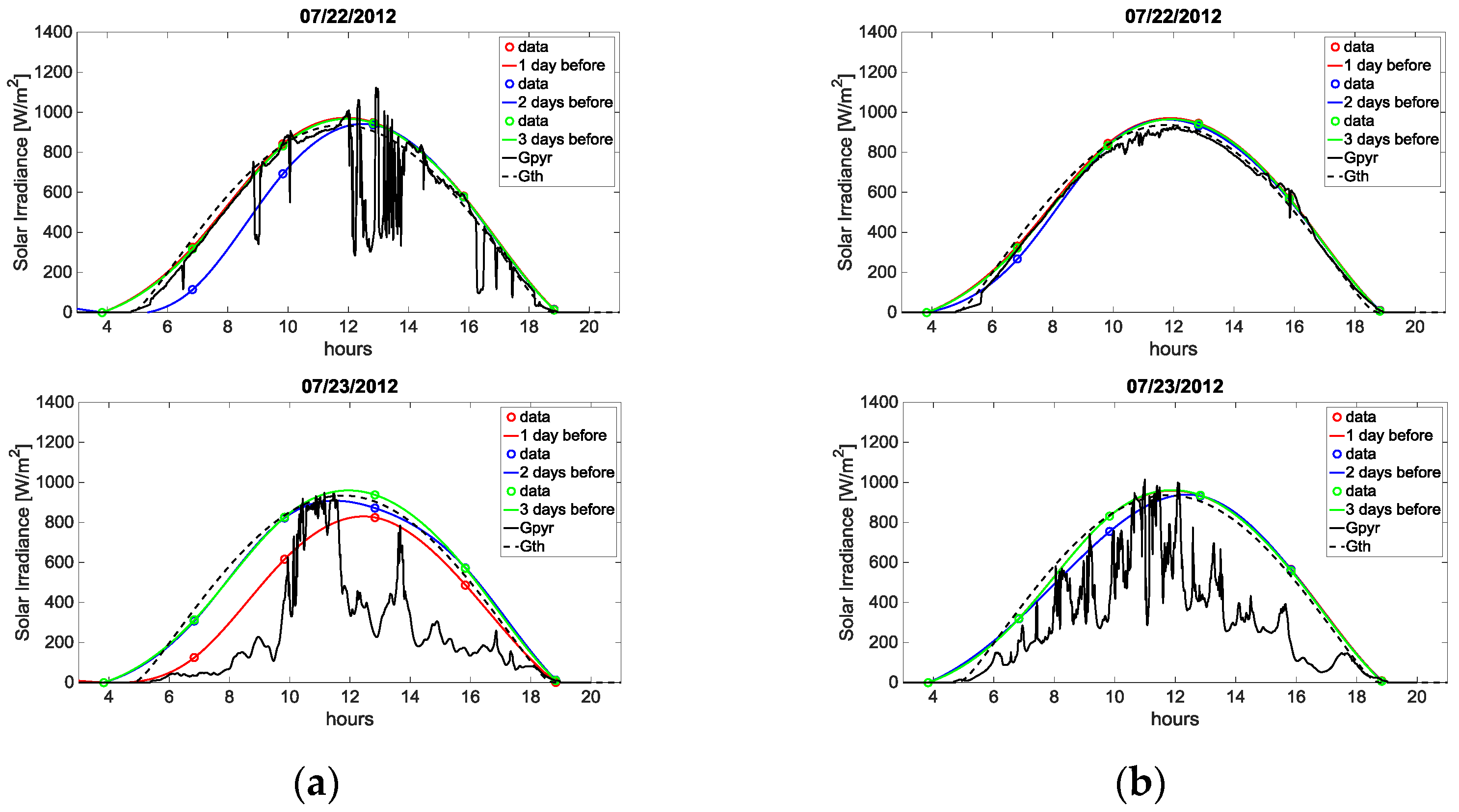
3.3. Comparison between Estimated Values and Measurements in the Two PV Sites

On the basis of Equation (10), the clearness index determines the amount of diffuse hourly irradiation with respect to the global hourly irradiation, and thus the sky conditions. The assessment of clear, variable and cloudy sky conditions is carried out for the pyranometer measurements and for the polynomial splines representing the estimated values. In both cases, the values are averaged at each hour. When the assessment for measurement and estimate indicates the same type of sky conditions, the comparison result is marked as a “pass”, otherwise it becomes a “fail”.
Table 2 and Table 3 report the comparison performance by showing the number of hours with correct classification (passes) and with incorrect classification (fails). The comparison is carried out with estimates referring to 1 day-ahead forecast, summarized for all the months of the year 2012 in the two sites. Only the hours having at least 30 min of sunlight are considered. The check on the sunlight hours is carried out for each day by using the clear sky model. The last row of each table reports the percentage of passes (or fails) per month related to the total number of sunlight hours per month.
For the site “Gi”, in summer (in particular in July) the highest number of hourly passes occurs for the variable condition. The cases classified as variable from the measurements but clear from the estimation occur mainly in the middle hours of the day (from 10 a.m. to 3 p.m.) in the days with greater occurrence of the ISBC effect. On the other hand, in spring a great number of hourly fails occur for the clear–variable condition.
The low number of clear days, especially in spring and summer, can be explained by the actual air turbidity. In general, the air pollution can play a fundamental role. The number of clear-sky days at the site “Ma” is lower than at the site “Gi”. In fact, the site “Ma” is close to high pollution areas, with the presence of fine dust in the air, produced by industrial steel mills.
Table 2. Number of passes for all the months of 2012.
(a) Site “Gi”
MeasuredEstimatedJanuaryFebruaryMarchAprilMayJuneJulyAugustSeptemberOctoberNovemberDecember
VariableVariable1928813680112139148130140120178185
ClearClear830519810812954109867755
CloudyCloudy73118331229101631453124
Total Passes207149205211232297212255257242214214
Passes %72%48%57%53%53%67%47%60%71%72%71%72%
(b) Site “Ma”
MeasuredEstimatedJanuaryFebruaryMarchAprilMayJuneJulyAugustSeptemberOctoberNovemberDecember
VariableVariable1659614570124113135141149124139155
ClearClear243144101118103507387771612
CloudyCloudy024183422901632451726
Total Passes189151207205244245185230268246172193
Passes %65%49%57%51%56%55%41%54%74%73%57%65%
Table 3. Number of fails for all the months of 2012.
(a) Site “Gi”
MeasuredEstimatedJanuaryFebruaryMarchAprilMayJuneJulyAugustSeptemberOctoberNovemberDecember
VariableClear376752590492514817
VariableCloudy187730776516574834305132
ClearVariable50591158312387757146462223
ClearCloudy8166219201612246
CloudyVariable200000000014
CloudyClear000000000000
Total Fails81159157188202148238169107928682
Fails %28%52%43%47%47%33%53%40%29%28%29%28%
(b) Site “Ma”
MeasuredEstimatedJanuaryFebruaryMarchAprilMayJuneJulyAugustSeptemberOctoberNovemberDecember
VariableClear126111212701206727323831
VariableCloudy307518777530664827258549
ClearVariable516611683967462764131215
ClearCloudy71010187241621008
CloudyVariable000400000122
CloudyClear000000000010
Total Fails1001571551941901982641939689128105
Fails %35%51%43%49%44%45%59%46%26%27%43%35%
Comparing the number of passes with the number of fails, it is interesting to point out that in both sites only in two months (February and July) the number of passes is lower than the number of fails. In particular, in July the classification of the cloudy conditions in these sites is particularly challenging, especially when a cloudy day appears after a number of successive clear days.

3.4. Identification of the Irradiance Spikes caused by Broken Clouds (ISBC) Conditions

In order to estimate the number of occurrences of the ISBC effect in a day, an additional control has been performed. In general, the ISBC effect may happen at each time (minute, hour…) of the day, when the irradiance spikes exceed the irradiance indicated by the reference model at clear sky. The maximum value of clear-sky irradiance changes in each day; the monthly values are shown in Table 4. The reference model considers a fixed plane (i.e., with the same 30° tilt angle of the modules in the PV plant).
Table 4. Maximum clear-sky solar irradiance values with tilted angle of 30° for each month of 2012.
MonthMax Clear-Sky Irradiance (W/m2) on a 30° Plane
Site “Gi”Site “Ma”
January852856
February971977
March10801100
April11001110
May10601070
June10601060
July10201030
August10801080
September10401040
October10001020
November906905
December856853
In this paper, a spike is defined by the occurrence of an increase in the global irradiance Gtcell on the tilted solar cells, from one minute to the successive minute, higher than a threshold value. The threshold is set to 45 W/m2, that is, the maximum expanded uncertainty of the pyranometer with 99.7% confidence indicated in Section 2.2. The occurrence of the ISBC effect has been determined by showing two different outcomes:
(i)
the number of irradiance spikes for which the measured irradiance exceeds the irradiance of the reference model at the same minute;
(ii)
the number of irradiance spikes for which the measured irradiance is so high to exceed the maximum irradiance Gmax indicated by the reference model of the corresponding day. The rationale of this choice is that for irradiance values higher than the maximum value established at clear-sky conditions the PV system may inject in the electrical network a power that could be even higher than the rated power of the PV plant.
For the two sites, the global irradiance Gtcell is gathered with a resolution of 1 min. For the “Gi” site, in the year 2012 the ISBC effect occurs for a number of minutes corresponding to about 2 days and 17 h. The details by month are shown in Table 5a. The occurrence of the ISBC effect in 2012 at the “Ma” site is similar to what happens at the “Gi” site, with a number of minutes in which the ISBC effect occurs corresponding to 2 days and 16 h. The details by month are shown in Table 5b. The months with a higher occurrence of the ISBC effect are in spring (April–May) and in autumn (September).
Table 5. Number of ISBC events for each month, considering Gtcell with time step of 1 min, exceeding the minute-by-minute points and the daily peak of the clear sky model.
Number of ISBC Events (Year 2012)
Month(a) Site “Gi”(b) Site “Ma”
Exceeding the Minute-by-Minute Points of the Clear Sky ModelExceeding the Daily Peak of the Clear Sky ModelExceeding the Minute-by-Minute Points of the Clear Sky ModelExceeding the Daily Peak of the Clear Sky Model
January378190357172
February228117231117
March23289430217
April552283469221
May646343397190
June25210820273
July22710416757
August154603410
September493207663311
October345161416166
November24512121479
December17486289140
Total year 3926186938691753

4. Accuracy of the Estimated Values

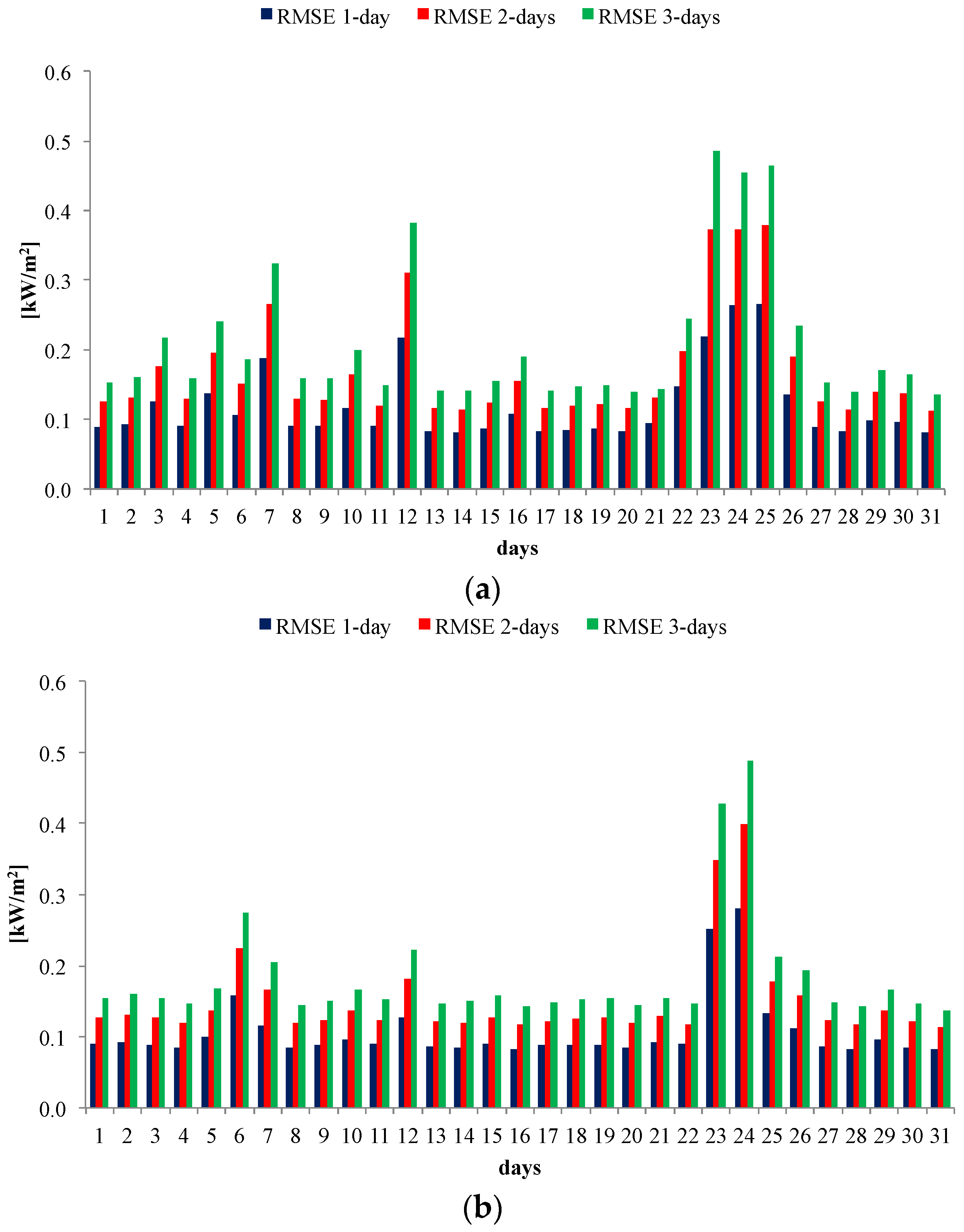
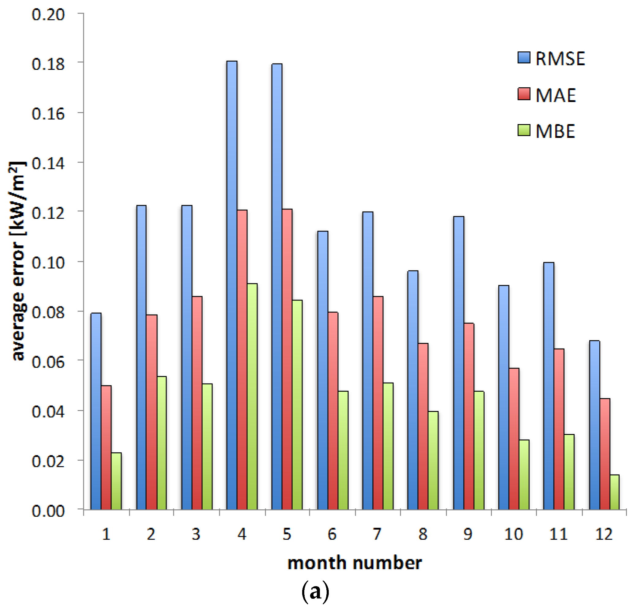
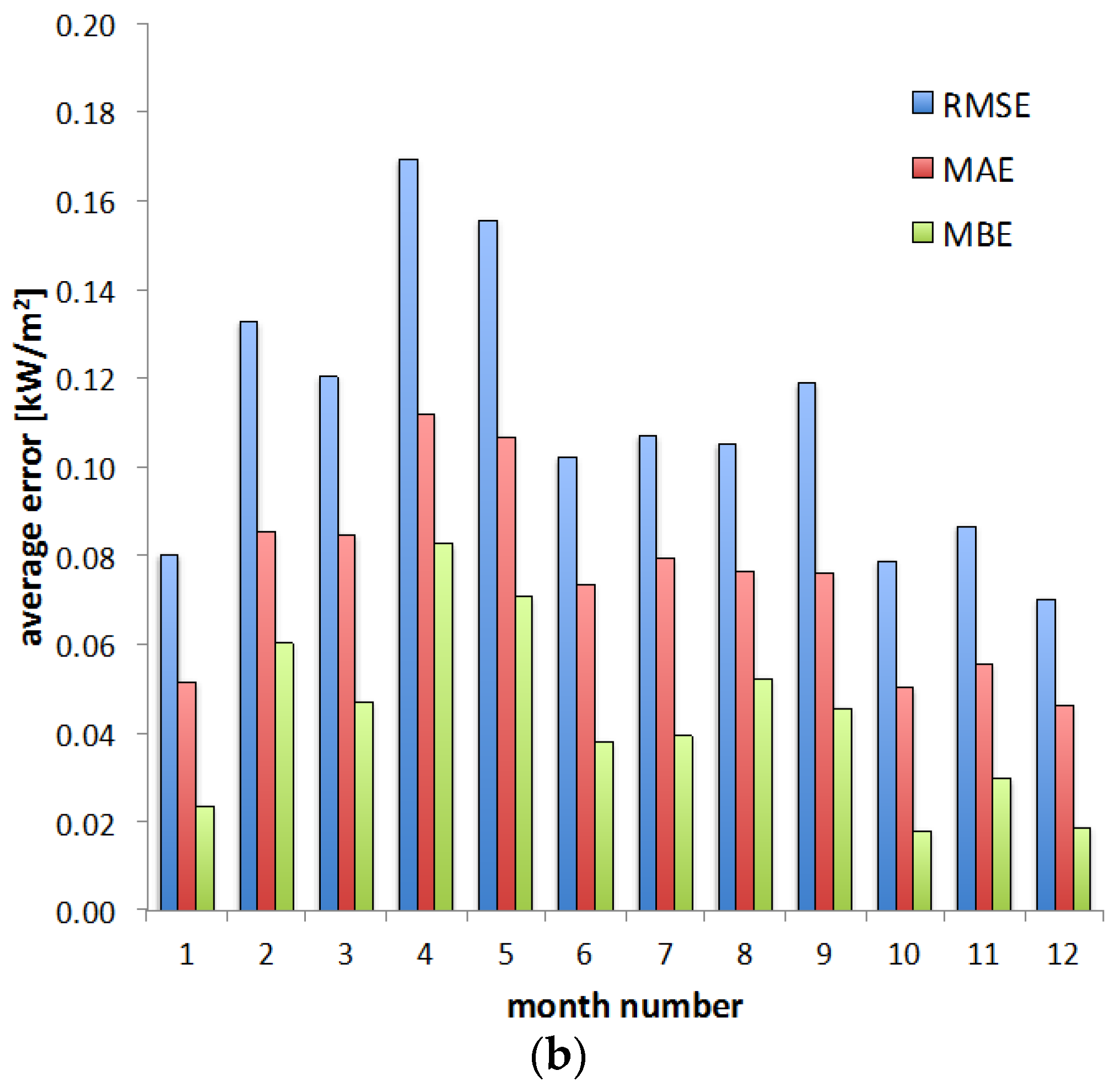
4.1. Error Indices to Compare the Irradiance Estimates with the Measurements

In order to compare the estimated quantities with the measured ones, the estimation error εG is the difference between the estimated irradiance Gest and the measured irradiance Gmeas [52]:
ε G = G e s t G m e a s
Different statistical parameters [53] have been calculated on a daily basis, by considering a generic error ε:
  • the root mean square error (RMSE):
    RMSE = 1 N i = 1 N ε i 2
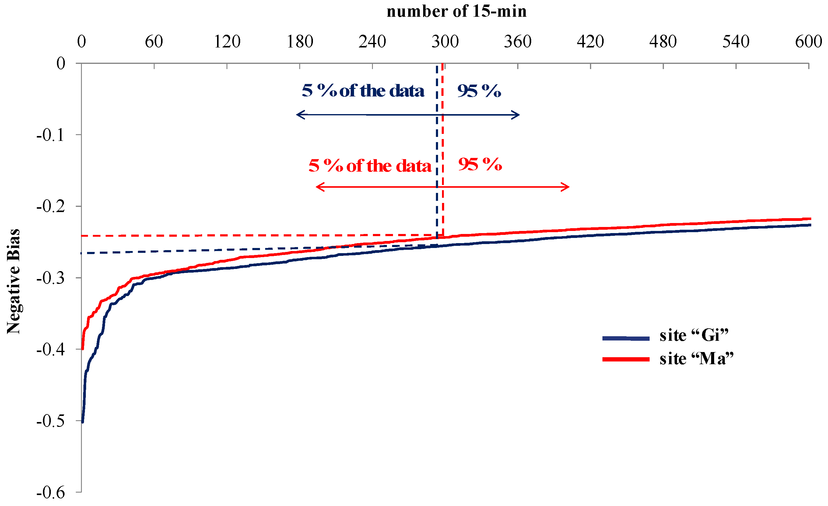
  • the mean bias error (MBE), representing the systematic part (bias) of the error [54]:
    MBE = ε ¯ = 1 N i = 1 N ε i
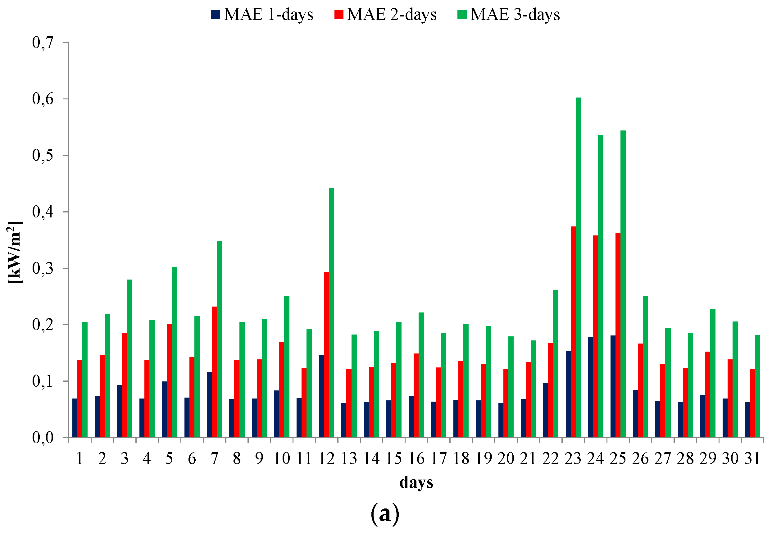
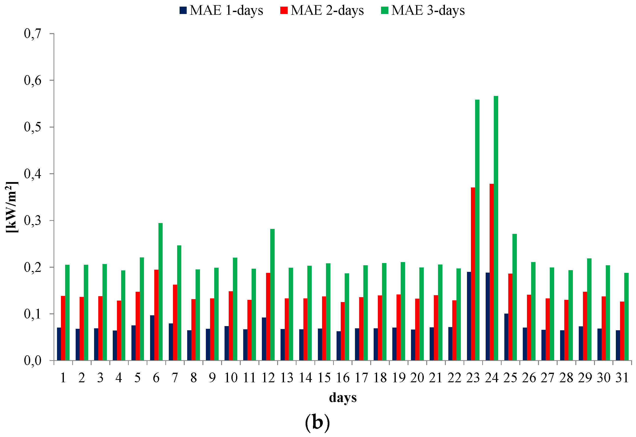
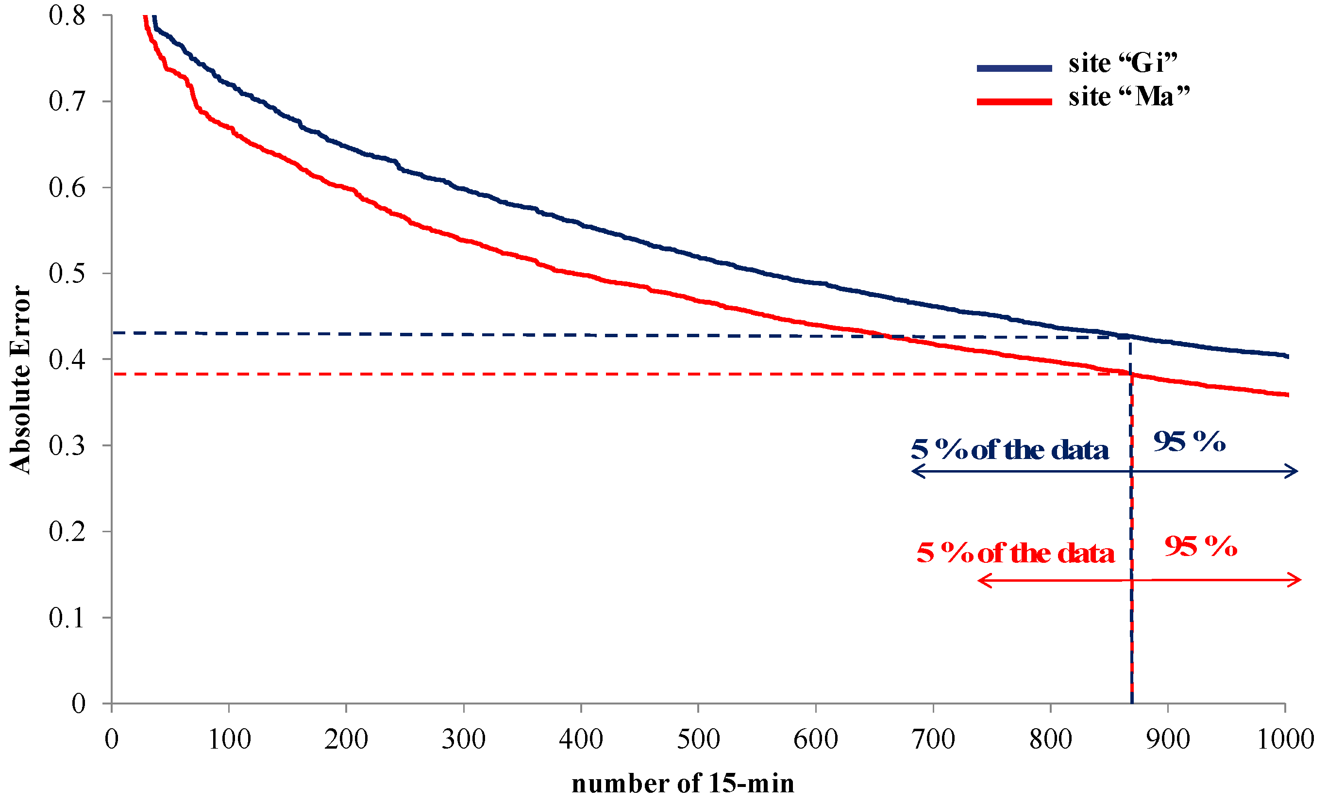
  • the mean absolute error (MAE):
    MAE = 1 N i = 1 N | ε i |
The estimation error is calculated by using Equation (11) with Gest given by the estimated data interpolated from the 1, 2 and 3 days-ahead irradiance forecasts, and Gmeas equal to the irradiance Gpyr measured from the pyranometer. Figure 3, Figure 4 and Figure 5 show the RMSE, the MBE and the MAE calculated errors, respectively, expressed in kW/m2 for the days of July 2012 in the sites “Gi” and “Ma”. For example, it can be observed that on 23 July there is a significant increase of the three errors with respect to the preceding days, at both sites. This situation can be explained by looking at the last graphs of Figure 2, in which the sky on 23 July becomes variable after a sequence of clearer days. A similar situation occurs on 24 July at both sites and on 25 July at the site “Gi”.
On the average, the 1-day ahead estimate is the most accurate, with lower errors compared to the 2-days and 3-days ahead estimates. In particular, considering the RMSE errors in Figure 3, the average value of the 1-day ahead estimates give figures around 119 W/m2 for the site “Gi” and around 107 W/m2 for the site “Ma”; whereas the maximum value is around 266 W/m2 for the site “Gi” and around 280 W/m2 for the site “Ma”. Furthermore, the minimum value is around 81 W/m2 for the site “Gi” and around 82 W/m2 for the site “Ma”. From Figure 4, it can be pointed out that the 1-day ahead estimates give MBE figures around 50 W/m2 for the site “Gi” and around 40 W/m2 for the site “Ma”. In the best results the MBE index decreases down to 20 W/m2 for the site “Gi” and down to 10 W/m2 for the site “Ma”, and in the worst results the MBE raises up to 140 W/m2 for the site “Gi” and up to 160 W/m2 for the site “Ma”. The presence of a positive bias (with estimates higher than the measured values) may be associated with air pollution. From Figure 5, the MAE for the 1-day ahead estimates is 90 W/m2 for the site “Gi” and 80 W/m2 for the site “Ma”, the minimum value is about 60 W/m2 for both sites and the maximum value is 180 W/m2 for the site “Gi” and 190 W/m2 for the site “Ma”.
Figure 3. The RMSE in kW/m2 in July. (a) Site “Gi”; (b) Site “Ma”.
Energies 09 00008 g003
Figure 4. The MBE in kW/m2 in July. (a) Site “Gi”; (b) Site “Ma”.
Energies 09 00008 g004
Figure 5. The MAE in kW/m2 in July. (a) Site “Gi”; (b) Site “Ma”.
Energies 09 00008 g005aEnergies 09 00008 g005b
In order to provide an overall view of the estimation errors during the year 2012, Figure 6 shows the monthly average values of the daily RMSE, MAE and MBE obtained from the 1 day-ahead estimates. At both sites, relatively high average errors occur in April and May, while generally the months with lower errors are from October to January. These results are consistent with the occurrence of the most relevant ISBC effects in April and May, as shown in Table 5.
Figure 6. Monthly average values of the daily RMSE, MAE and MBE obtained from the 1-day ahead estimates at the two sites. (a) Site “Gi”; (b) Site “Ma”.
Energies 09 00008 g006aEnergies 09 00008 g006b

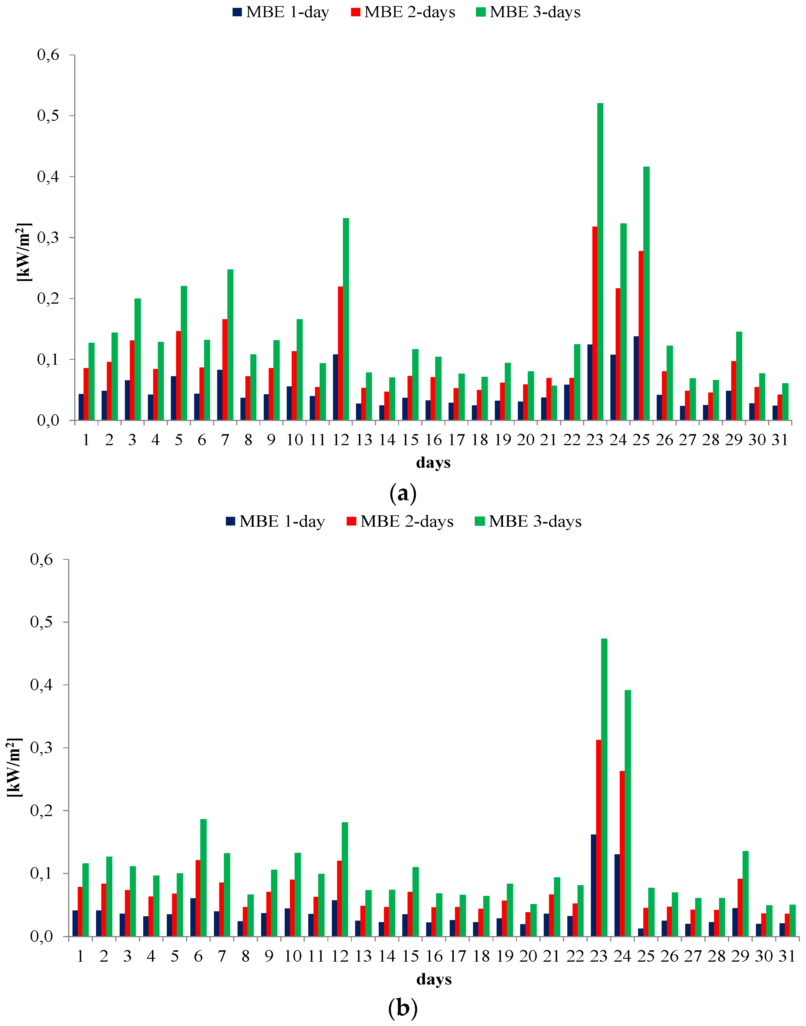
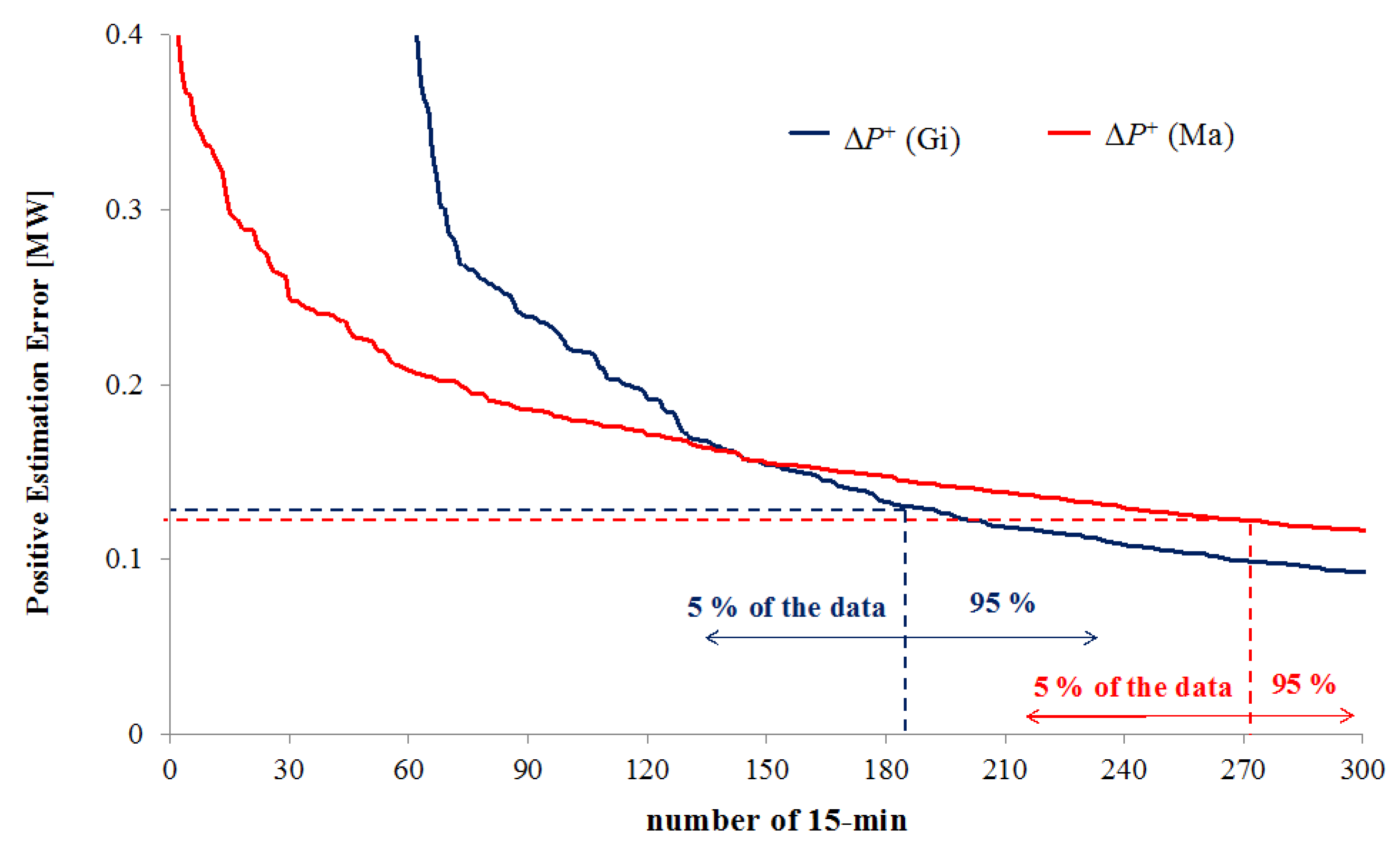
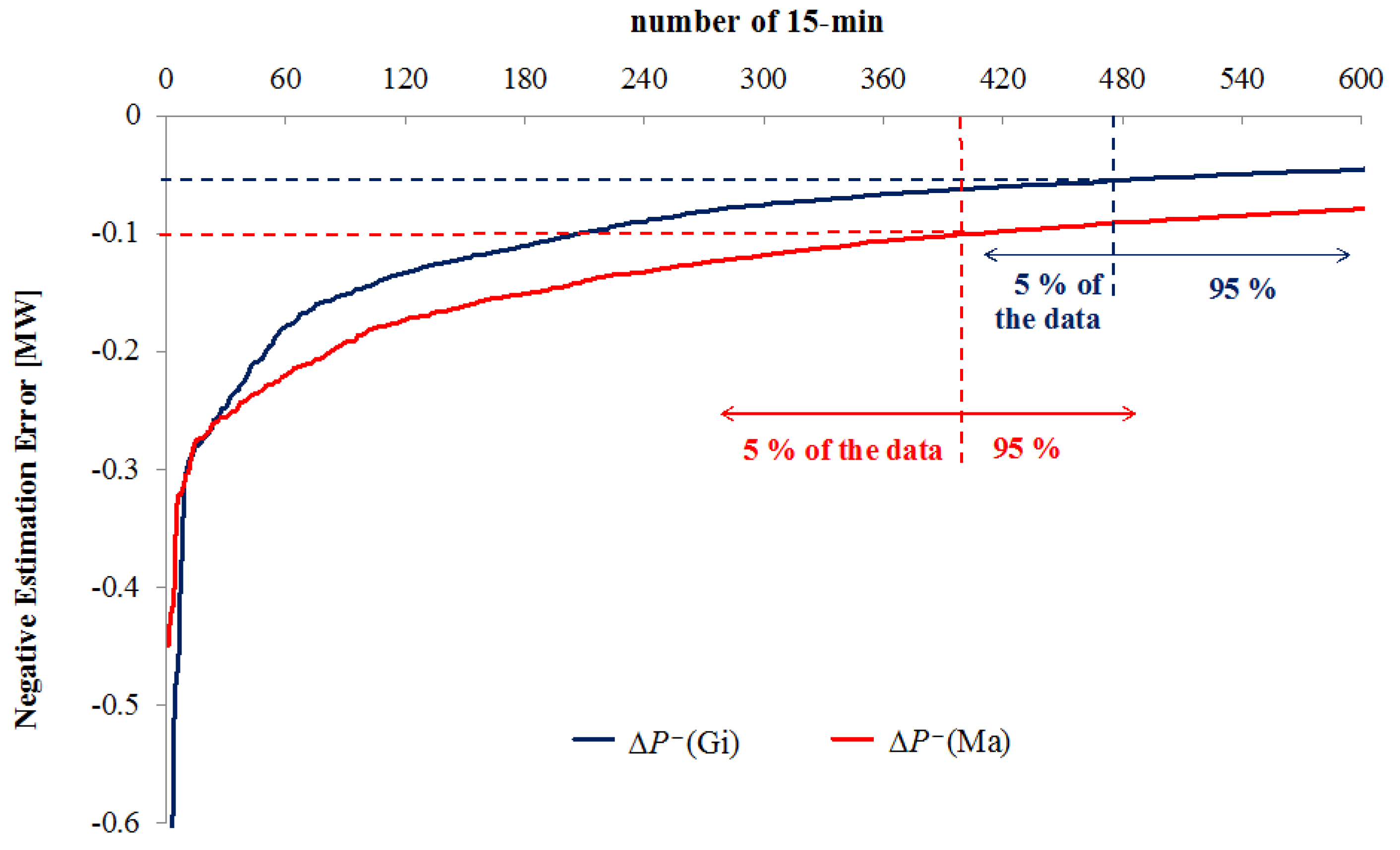
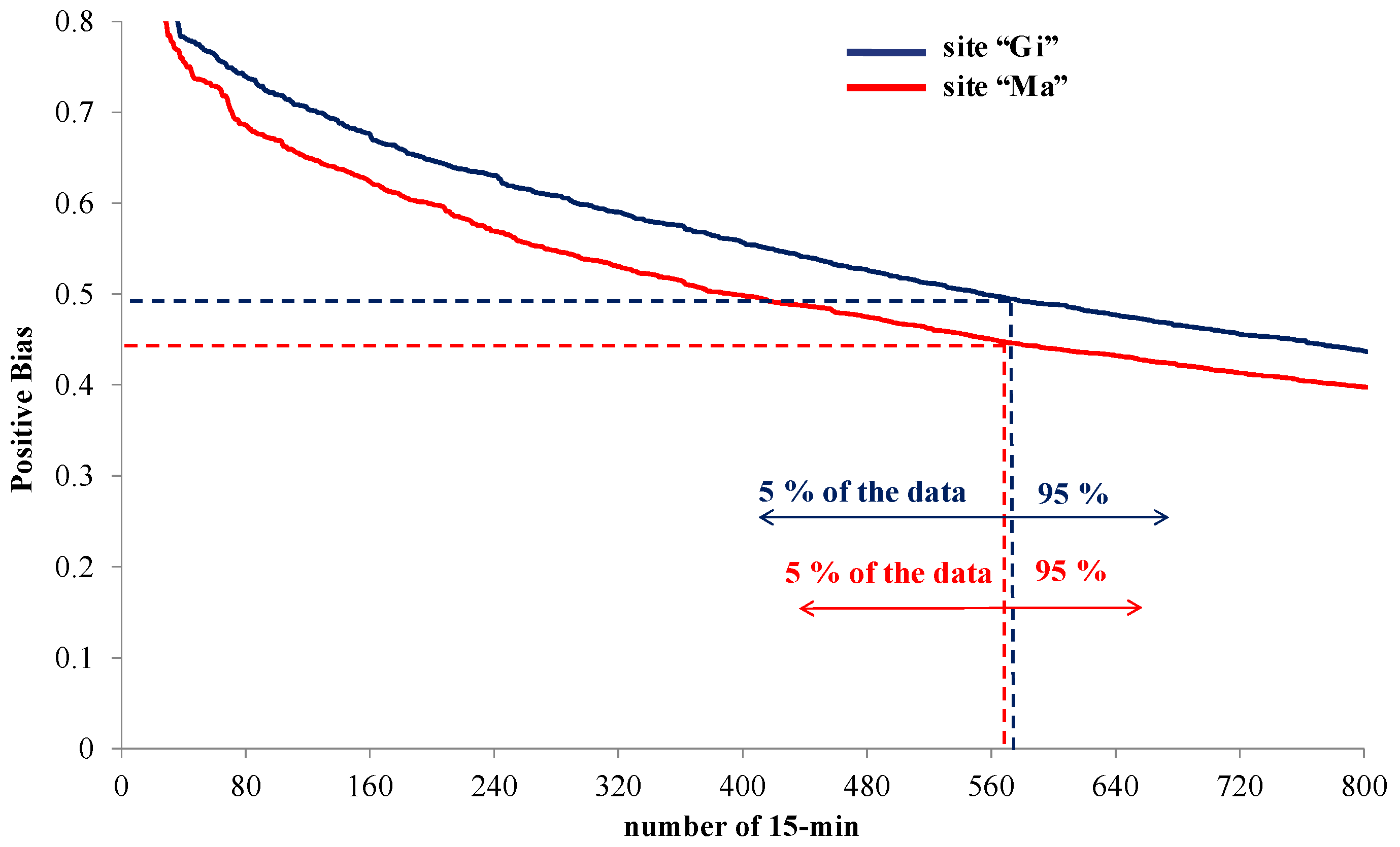
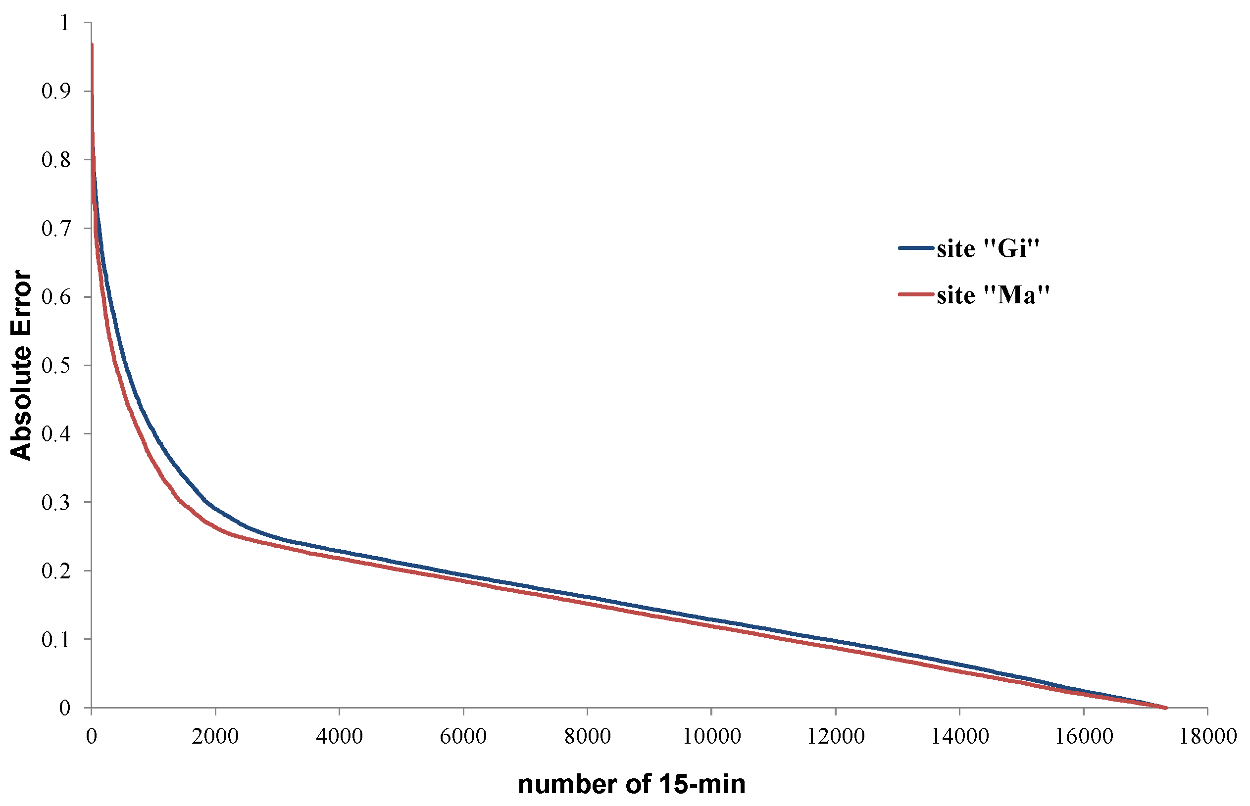
4.2. Duration Curves of Bias and Absolute Error

The figures reported in this section show the error duration curves for the sites “Gi” and “Ma”, representing the bias and the absolute errors of the estimates referring to the 1 day-ahead forecast with respect to the irradiance measurements. The data are averaged at 15-min time steps for one year. As renewable sources are rapidly gaining a larger share of the market, the importance of forecasting their productivity is essential for grid operators who have always to balance electricity supply and demand. The evaluation of the forecast errors is helpful for the grid operator, for example, to estimate to what extent the contribution of PV plants to the grid-connected local generation (calculated by using the 1 day-ahead forecast data) can be trustable.
Figure 7 shows the error duration curves of positive and negative bias, where positive biases correspond to estimates higher than the measurements, and vice versa. The errors are expressed in per units by considering a reference value of 1 kW/m2. For both sites, the number of positive bias entries is higher than the number of negative bias entries, indicating a major trend to overestimate the irradiance values in these cases. This overestimation issue deserves some attention. In fact, using the estimated irradiance values as input data to estimate the PV power generation, an overestimation of the PV production creates an undue imbalance between the actual generation and the load. This imbalance impacts on the need to procure further reserves for supporting the grid operation.
Figure 8 indicates that the positive bias exceeded by 5% of the quarters of hour during the year is about 0.49 for the site “Gi”, and about 0.44 for the site “Ma”. Figure 9 shows that the negative bias exceeded by 5% of the quarters of hour during the year is about −0.24 for the site “Gi”, and about −0.27 for the site “Ma”. Furthermore, Figure 10 shows the duration curves for the absolute error. In the zoom of Figure 11 it is shown that the absolute error exceeded by 5% of the quarters of hour during the year is about 0.43 for the site “Gi” and about 0.38 for the site “Ma”.
The bias and error values obtained are compared with the pyranometer uncertainty indicated in Section 2.2. The absolute error exceeded in 5% of the cases is indicatively one order of magnitude higher than the expanded uncertainty (45 W/m2, that is, 0.045 per units) of the pyranometer at confidence level 99.7%. Thereby, the measurement uncertainty plays a minor role in the interpretation of the results.
Figure 7. Duration curve of positive and negative bias for the solar irradiance estimated data with respect to measurements for the year 2012. (a) Site “Gi”; (b) Site “Ma”.
Energies 09 00008 g007
Figure 8. Zoom of the duration curves of positive bias for the solar irradiance estimated data with respect to measurements for the year 2012 at the sites “Gi” and “Ma”.
Energies 09 00008 g008
Figure 9. Zoom of the duration curves of negative bias for the solar irradiance estimated data with respect to measurements for the year 2012 at the sites “Gi” and “Ma”.
Energies 09 00008 g009
Figure 10. Duration curve of the absolute errors for the solar irradiance estimated data with respect to measurements for the year 2012.
Energies 09 00008 g010
Figure 11. Zoom of the duration curves of the absolute error for the solar irradiance estimated data with respect to measurements for the year 2012 at the sites “Gi” and “Ma”.
Energies 09 00008 g011

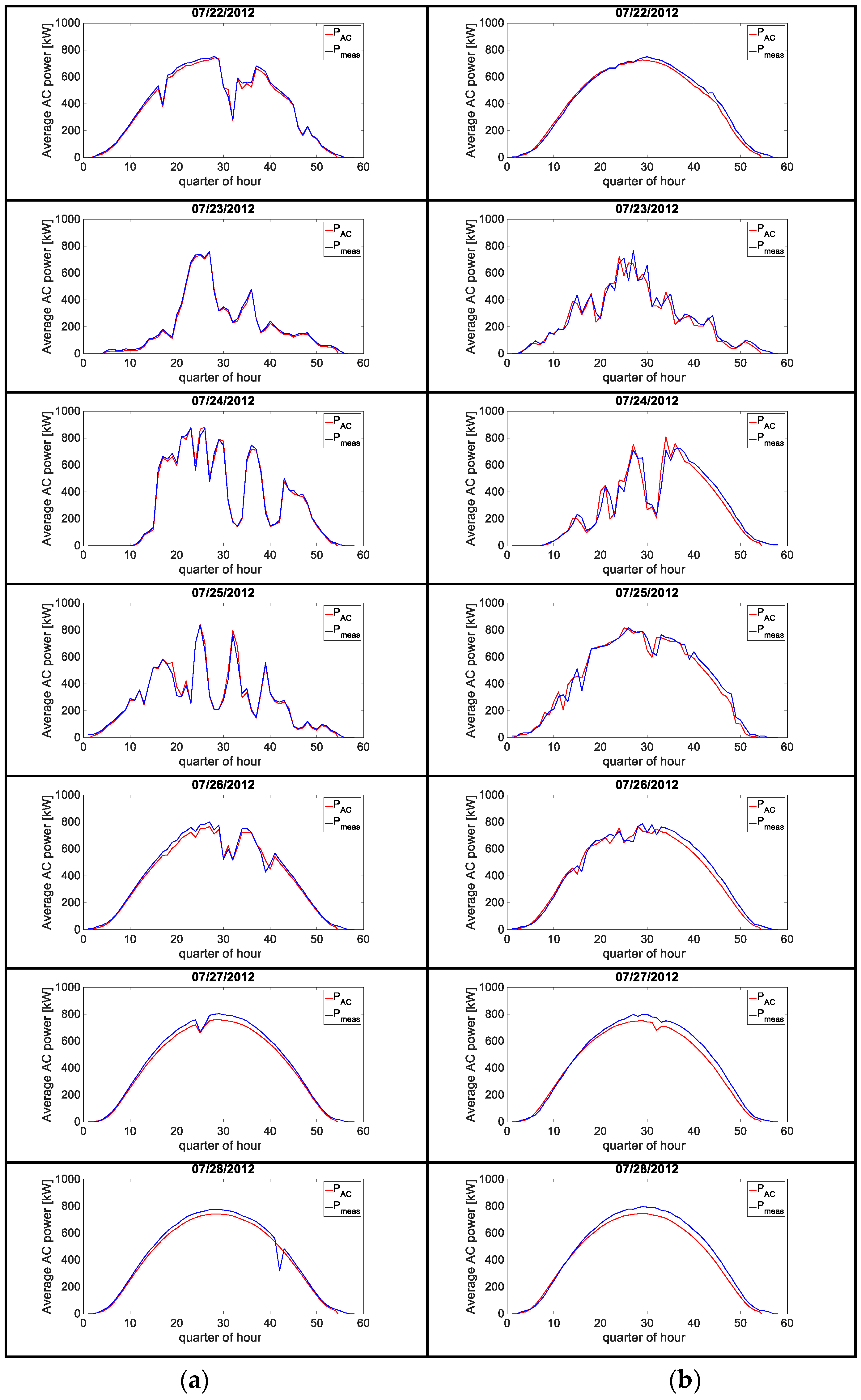
5. AC Power Estimations Compared with Experimental Results

Figure 12 shows the application of the PV conversion model to the reference-cell irradiance data for seven consecutive days of July 2012 in the sites “Gi” and “Ma”. For example, low deviations occur on 23 July (an extremely variable day), meaning that the model is able to follow also huge irradiance variations. Moreover, thanks to the days with clear sky, since the deviations are proportional to the solar irradiance, it is possible to detect the failure of a portion of the PV arrays, becoming evident by the occurrence of large and regular deviations between the measured values and the outputs of the model, as reported in [20]. Thereby, a salient characteristic of the model is that it can be useful for fault diagnosis.
Figure 12. Comparison between PV power measurements and simulations for seven consecutive days of July 2012. (a) Site “Gi”; (b) Site “Ma”.
Energies 09 00008 g012
The differences appearing in Figure 12 may be also attributed to the fact that average values have been used in the representation of the sources of losses and efficiencies, with the scope of estimating both clear sky and variable conditions without varying the efficiencies in function of the sky conditions.
For the calculation of the power PAC to be used in Equation (9), the reference-cell irradiance data gathered on the tilted plane Gtcell, averaged on 15-min basis, are used as inputs of the model previously described. The results of error calculation for the estimated power profiles are reported in the following figures. The error duration curves calculated for ΔP are represented with averaging time step of 15 min and on an annual basis. Figure 13 shows the duration curves of positive and negative ΔP errors. At both sites, the number of negative errors ΔP is higher than the number of positive errors ΔP+, but the positive errors may be quantitatively higher. This aspect is confirmed by comparing the results shown in the zoom of Figure 14 (for positive estimation errors) and Figure 15 (for negative estimation errors). The corresponding errors exceeded by 5% of the number of quarters of hour in one year are of about 120–130 kW for the positive errors at the two sites, and of about −60 kW and −100 kW for the negative errors at the sites “Gi” and “Ma”, respectively.
Figure 13. Duration curve of positive and negative estimation errors of the AC power profiles with respect to experimental results for the year 2012. (a) Site “Gi”; (b) Site “Ma”.
Energies 09 00008 g013
Figure 14. Zoom of the duration curves of positive estimation errors of the AC power profiles with respect to experimental results for the year 2012 at the sites “Gi” and “Ma”.
Energies 09 00008 g014
Figure 15. Zoom of the duration curves of negative estimation errors of the AC power profiles with respect to experimental results for the year 2012 at the sites “Gi” and “Ma”.
Energies 09 00008 g015

6. Conclusions

This paper has presented the comparison of irradiance and AC power estimates with respect to the experimental results gathered from meteorological stations and energy meters in grid-connected PV systems. The data used refer to two PV sites located in Southern Italy. The solar irradiance forecasts up to 3 days ahead on the horizontal plane, available from a weather forecast provider at geographic coordinates close to the PV plants, have been used to obtain estimated data patterns. It has been established to what extent the estimated data referring to the 1 day-ahead forecast are better than the estimated data determined from the 2 and 3 days-ahead forecasts, by calculating some classical average errors. A method to classify each hour of a day by using three categories (variable, cloudy, or clear) has been implemented. Examining the results month by month, it has been possible to determine the number of successful and unsuccessful classifications provided by the 1 day-ahead estimated data with respect to the pyranometer measurements. The low number of clear-sky days, especially in spring and summer, can be explained by the air turbidity, e.g., due to pollution deriving from human activities. Deep cloudy weather cases can be reproduced when the WRF forecasts indicate low irradiance values and the polynomial spline connecting these points remains well below the clear sky conditions.
The results obtained for the ISBC effect have shown that this particular effect contributes to determine variable sky conditions. Assessing the ISBC effect is useful to explain the presence of power production peaks even higher than the rated power specified at STC of irradiance and cell temperature. The ISBC effect, even if noticeable on 1-min scale, is smoothed on the 15-min scale and considering the aggregation of more locations.
For the comparison between estimated and measured data, the statistical indicators RMSE, MAE and MBE have been calculated. Considering positive and negative MBE, the error duration curves have been obtained for 15-min averaged irradiance values on an annual basis. Finally, the combination of irradiance estimation and PV conversion model provides interesting results to boost the PV penetration into the grid. Considering the error of the AC power calculated from the PV model with respect to the AC power measured by the meters on the real grid-connected PV system, the error duration curve allows us determine which positive or negative errors occur for an established percentage of the data analyzed.
The categorization of the types of sky for each period of the day, associated with the short-term estimation of the weather conditions, is a specific information that can be used to quantify the additional reserve necessary to balance the fluctuations of the PV generation in periods in which high fluctuations are expected, without requiring such reserve to be continuously available [55,56]. The connection of PV power to the grid, like in the case of wind power, requires additional reserve with respect to the normal reserve required for the balance control of the grid [57]. For this purpose, the information on the PV forecasting uncertainty can be handled to assist the assessment of the amount of reserves needed to integrate the uncertain PV generation into the electrical system. For this purpose, persistence models, Markov chains and neural networks can be applied [56,57,58]. These results are also useful to estimate the contribution of PV in the definition of capacity value and capacity credit of renewable energy sources [59,60,61].

Acknowledgments

Part of the research leading to these results has received funding from the European Union Seventh Framework Programme FP7 under grant agreement No. 309048, project SiNGULAR (Smart and Sustainable Insular Electricity Grids Under Large-Scale Renewable Integration).

Author Contributions

The authors contributed equally to the work.

Conflicts of Interest

The authors declare no conflict of interest.

References

  1. Jensenius, J.S. Solar Resources. In Insolation Forecasting; Massachusetts Institute of Technology (MIT) Press: Cambridge, MA, USA, 1989; pp. 335–349. [Google Scholar]
  2. Glahn, H.R.; Lowry, D.A. The use of model output statistics (MOS) in objective weather forecasting. Appl. Meteorol. 1972, 11, 1203–1211. [Google Scholar] [CrossRef]
  3. Kaifel, A.K.; Jesemann, P. An adaptive filtering algorithm for very short-range forecast of cloudiness applied to meteosat data. In Proceedings of the 9th Meteosat Scientific Users Meeting, Locarno, Switzerland, 15–18 September 1992.
  4. Beyer, H.G.; Costanzo, C.; Heinemann, D.; Reise, C. Short range forecast of PV energy production using satellite image analysis. In Proceedings of the 12th European Photovoltaic Solar Energy Conference, Amsterdam, The Netherlands, 11–15 April 1994; pp. 1718–1721.
  5. Kang, B.O.; Tam, K. New and improved methods to estimate day-ahead quantity and quality of solar irradiance. Appl. Energy 2015, 137, 240–249. [Google Scholar] [CrossRef]
  6. Huld, T.; Amillo, A. Estimating PV module performance over large geographical regions: The role of irradiance, air temperature, wind speed and solar spectrum. Energies 2015, 8, 5159–5181. [Google Scholar] [CrossRef] [Green Version]
  7. Mellit, A.; Massi Pavan, A. Performance prediction of 20 kWp grid-connected photovoltaic plant at Trieste (Italy) using artificial neural network. Energy Convers. Manag. 2010, 51, 2431–2441. [Google Scholar] [CrossRef]
  8. Mellit, A.; Massi Pavan, A. A 24-h forecast of solar irradiance using artificial neural network: Application for performance prediction of a grid-connected PV plant at Trieste, Italy. Sol. Energy 2010, 84, 807–821. [Google Scholar] [CrossRef]
  9. Izgi, E.; Oztopal, A.; Yerli, B.; Kaymak, M.K.; Sahin, A.D. Short-mid-term solar power prediction by using artificial neural networks. Sol. Energy 2012, 86, 725–733. [Google Scholar] [CrossRef]
  10. Da Silva Fonseca, J.G., Jr.; Oozeki, T.; Takashima, T.; Koshimizu, G.; Uchida, Y.; Ogimoto, K. Use of support vector regression and numerically predicted cloudiness to forecast power output of a photovoltaic power plant in Kitakyushu, Japan. Progress Photovolt. Res. Appl. 2011, 20, 874–882. [Google Scholar] [CrossRef]
  11. Shi, J.; Lee, W.; Liu, Y.; Yang, Y.; Wang, P. Forecasting power output of photovoltaic systems based on weather classification and support vector machines. IEEE Trans. Ind. Appl. 2012, 48, 1064–1069. [Google Scholar] [CrossRef]
  12. Bouzerdoum, M.; Mellit, A.; Massi Pavan, A. A hybrid model (SARIMA–SVM) for short-term power forecasting of a small-scale grid-connected photovoltaic plant. Sol. Energy 2013, 98, 226–235. [Google Scholar] [CrossRef]
  13. Pelland, S.; Galanis, G.; Kallos, G. Solar and photovoltaic forecasting through post-processing of the global environmental multiscale numerical weather prediction model. Progress Photovolt. Res. Appl. 2011, 21, 284–296. [Google Scholar] [CrossRef]
  14. Cai, T.; Duan, S.; Chen, C. Forecasting power output for grid-connected photovoltaic power system without using solar radiation measurement. In Proceedings of the 2nd IEEE International Symposium on Power Electronics for Distributed Generation Systems (PEDG), Hefei, China, 16–18 June 2010.
  15. Bessa, R.J.; Trindade, A.; Miranda, V. Spatial-temporal solar power forecasting for smart grids. IEEE Trans. Ind. Inform. 2015, 11, 232–241. [Google Scholar] [CrossRef]
  16. Dambreville, R.; Blanc, P.; Chanussot, J.; Boldo, D. Very short term forecasting of the global horizontal irradiance using a spatio-temporal autoregressive model. Renew. Energy 2014, 72, 291–300. [Google Scholar] [CrossRef]
  17. Iqbal, M. An introduction to solar radiation; Academic Press: Toronto, ON, Canada, 1983. [Google Scholar]
  18. Duffie, J.A.; Beckman, W.A. Solar Engineering of Thermal Processes, 2nd ed.; Wiley Interscience: New York, NY, USA, 1991. [Google Scholar]
  19. Şen, Z. Solar Energy Fundamentals and Modeling Techniques; Springer: Berlin, Germany, 2008; pp. 70–71. [Google Scholar]
  20. The American Society of Heating, Refrigerating and Air-Conditioning Engineers (ASHRAE). Handbook of Fundamentals, American Society of Heating, Refrigeration and Air-Conditioning Engineers; ASHRAE: Atlanta, GA, USA, 1993. [Google Scholar]
  21. Moon, P.; Spencer, D.E. Illumination from a non uniform sky. Illum. Eng. 1942, 37, 707–726. [Google Scholar]
  22. Chicco, G.; Cocina, V.; Spertino, F. Characterization of solar irradiance profiles for photovoltaic system studies through data rescaling in time and amplitude. In Proceedings of the 49th International Universities’ Power Engineering Conference (UPEC 2014), Cluj-Napoca, Romania, 2–5 September 2014.
  23. Joint Research Centre of the European Commission, Photovoltaic Geographical Information System (PVGIS). Available online: http://re.jrc.ec.europa.eu/pvgis/apps4/pvest.php (accessed on 16 December 2015).
  24. Spertino, F.; di Leo, P.; Cocina, V. Accurate measurements of solar irradiance for evaluation of photovoltaic power profiles. In Proceedings of the IEEE Conference Powertech, Grenoble, France, 16–20 June 2013; pp. 1–5.
  25. Czekalski, D.; Chochowski, A.; Obstawski, P. Parameterization of daily solar irradiance variability. Renew. Sustain. Energy Rev. 2012, 16, 2461–2467. [Google Scholar] [CrossRef]
  26. Badosa, J.; Haeffelin, M.; Chepfer, H. Scales of spatial and temporal variation of solar irradiance on Reunion tropical island. Sol. Energy 2013, 88, 42–56. [Google Scholar] [CrossRef]
  27. Chicco, G.; Cocina, V.; di Leo, P.; Spertino, F. Weather forecast-based power predictions and experimental results from photovoltaic systems. In Proceedings of the IEEE Conference Speedam, Ischia, Italy, 18–20 June 2014.
  28. International Organization for Standardization (ISO). Solar Energy—Specification and Classification of Instruments for Measuring Hemispherical Solar and Direct Solar Radiation; ISO 9060:1990; ISO: Geneva, Switzerland, 1990. [Google Scholar]
  29. Carullo, A.; Ferraris, F.; Vallan, A.; Spertino, F.; Attivissimo, F. Uncertainty analysis of degradation parameters estimated in long-term monitoring of photovoltaic plants. Measurement 2014, 55, 641–649. [Google Scholar] [CrossRef]
  30. Reinders, A.H.M.E.; van Dijk, V.A.P.; Wiemken, E.; Turkenburg, W.C. Technical and economic analysis of grid-connected PV systems by means of simulation. Progress Photovolt. Res. Appl. 1999, 7, 71–82. [Google Scholar] [CrossRef]
  31. Markvart, T. Solar Electricity, 2nd ed.; John Wiley & Sons: Hoboken, NJ, USA, 2000. [Google Scholar]
  32. International Electrotechnical Commission (IEC). Crystalline Silicon Photovoltaic (PV) Array. On-Site Measurement of I-V Characteristics; IEC 61829; British Standards Institution: Geneva, Switzerland, 1998. [Google Scholar]
  33. Spertino, F.; Sumaili Akilimali, J. Are manufacturing I-V mismatch and reverse currents key factors in large photovoltaic arrays? IEEE Trans. Ind. Electron. 2009, 56, 4520–4531. [Google Scholar] [CrossRef]
  34. Spertino, F.; Corona, F. Monitoring and checking of performance in photovoltaic plants: A tool for design, installation and maintenance of grid-connected systems. Renew. Energy 2013, 60, 722–732. [Google Scholar] [CrossRef]
  35. Spertino, F.; Corona, F.; di Leo, P. Limits of advisability for master-slave configuration of DC-AC converters in photovoltaic systems. IEEE J. Photovolt. 2012, 2, 547–554. [Google Scholar] [CrossRef]
  36. Tapakis, R.; Charalambides, A.G. Equipment and methodologies for cloud detection and classification: A review. Sol. Energy 2013, 95, 392–430. [Google Scholar] [CrossRef]
  37. De Miguel, A.; Bilbao, J.; Aguiar, R.; Kambezidis, H.; Negro, E. Diffuse solar irradiation model evaluation in the North Mediterranean Belt area. Sol. Energy 2001, 70, 143–153. [Google Scholar] [CrossRef]
  38. Erbs, D.G.; Kein, S.A.; Duffie, J.A. Estimation of the diffuse radiation fraction for hourly, daily and monthly-average global radiation. Sol. Energy 1982, 28, 293–302. [Google Scholar] [CrossRef]
  39. Orgill, J.F.; Hollands, K.G.T. Correlation equation for hourly diffuse radiation on a horizontal surface. Sol. Energy 1977, 19, 357–359. [Google Scholar] [CrossRef]
  40. Iqbal, M. Prediction of hourly diffuse solar radiation from measured hourly global radiation on a horizontal surface. Sol. Energy 1980, 24, 491–503. [Google Scholar] [CrossRef]
  41. Lorenz, E.; Heinemann, D. Prediction of solar irradiance and photovoltaic power. Compr. Renew. Energy 2012, 1, 239–292. [Google Scholar]
  42. Meteorological Service of Catalonia, Meteo.Cat. Available online: http://www.meteo.cat (accessed on 16 December 2015).
  43. The Weather Research & Forecasting Model. Available online: http://www.wrf-model.org (accessed on 16 December 2015).
  44. Cocina, V. Economy of Grid-Connected Photovoltaic Systems and Comparison of Irradiance/Electric Power Predictions vs. Experimental Results. Ph.D. Thesis, Politecnico di Torino, Torino, Italy, 2014. [Google Scholar]
  45. Sluiter, R. Interpolation methods for climate data. Literature review. KNMI (Koninklijk Nederlands Meteorologisch Instituut) intern rapport IR 2009-04. De Bilt, The Netherlands, 19 November 2008.
  46. Estupiñán, J.G.; Raman, S.; Crescenti, G.H.; Streicher, J.J.; Barnard, W.F. Effects of clouds and haze on UV-B radiation. J. Geophys. Res. 1996, 101, 16807–16816. [Google Scholar] [CrossRef]
  47. Craig, F.; Bohren, C.F.; Clothiaux, E.E. Fundamentals of Atmospheric Radiation; Wiley-VCH: Weinheim, Germany, 2006. [Google Scholar]
  48. Morf, H. A stochastic solar irradiance model adjusted on the Ångström-Prescott regression. Sol. Energy 2013, 87, 1–21. [Google Scholar] [CrossRef]
  49. Luoma, J.; Kleissl, J.; Murray, K. Optimal inverter sizing considering cloud enhancement. Sol. Energy 2012, 86, 421–429. [Google Scholar] [CrossRef]
  50. Wirth, G.; Lorenz, E.; Spring, A.; Becker, G.; Pardatscher, R.; Witzmann, R. Modeling the maximum power output of a distributed PV fleet. Progress Photovolt. Res. Appl. 2015, 23, 1164–1181. [Google Scholar] [CrossRef]
  51. Yordanov, G.H.; Midtgård, O.-M.; Saetre, T.O.; Nielsen, H.K.; Norum, L.E. Overirradiance (Cloud Enhancement) events at high latitudes. IEEE J. Photovolt. 2013, 3, 271–277. [Google Scholar] [CrossRef]
  52. Lorenz, E.; Hurka, J.; Heinemann, D.; Beyer, H.G. Irradiance forecasting for the power prediction of grid-connected photovoltaic systems. IEEE J. Sel. Top. Appl. Earth Obs. Remote Sens. 2009, 2, 2–10. [Google Scholar] [CrossRef]
  53. IEA (International Energy Agency). Photovoltaic and solar forecasting: State of the art. In Report IEA Photovoltaic Power Systems Programme (PVPS) T14; IEA: St. Ursen, Switzerland, 2013; Volume 1, pp. 1–36. [Google Scholar]
  54. Diagne, M.; David, M.; Lauret, P.; Boland, J.; Schmutz, N. Review of solar irradiance forecasting methods and a proposition for small-scale insular grids. Renew. Sustain. Energy Rev. 2013, 27, 65–76. [Google Scholar] [CrossRef]
  55. Nijhuis, M.; Rawn, B.; Gibescu, M. Prediction of power fluctuation classes for photovoltaic installations and potential benefits of dynamic reserve allocation. IET Renew. Power Gener. 2014, 8, 314–323. [Google Scholar] [CrossRef]
  56. Yan, X.; Francois, B.; Abbes, D. Operating power reserve quantification through PV generation uncertainty analysis of a microgrid. In Proceedings of the IEEE PowerTech, Eindhoven, The Netherlands, 29 June–2 July 2015.
  57. Brouwer, A.S.; van den Broek, M.; Seebregts, A.; Faaij, A. Impacts of large-scale intermittent renewable energy sources on electricity systems, and how these can be modeled. Renew. Sustain. Energy Rev. 2014, 33, 443–466. [Google Scholar] [CrossRef]
  58. Tabone, M.D.; Callaway, D.S. Modeling variability and uncertainty of photovoltaic generation: A hidden state spatial statistical approach. IEEE Trans. Power Syst. 2015, 30, 2965–2973. [Google Scholar] [CrossRef]
  59. Perez, R.; Taylor, M.; Hoff, T.; Ross, J.P. Reaching consensus in the definition of photovoltaics capacity credit in the USA: A practical application of satellite-derived solar resource data. IEEE J. Sel. Top. Appl. Earth Obs. Remote Sens. 2008, 1, 28–33. [Google Scholar] [CrossRef]
  60. Simoglou, C.K.; Biskas, P.N.; Bakirtzis, E.A.; Matenli, A.N.; Petridis, A.I.; Bakirtzis, A.G. Evaluation of the capacity credit of RES: The Greek case. In Proceedings of the IEEE PowerTech, Grenoble, France, 16–20 June 2013.
  61. Munoz, F.D.; Mills, A.D. Endogenous assessment of the capacity value of solar PV in generation investment planning studies. IEEE Trans. Sustain. Energy 2015, 6, 1574–1585. [Google Scholar] [CrossRef]

