
Two-Dimensional Simulation of Mass Transfer in Unitized Regenerative Fuel Cells under Operation Mode Switching

Abstract
:1. Introduction
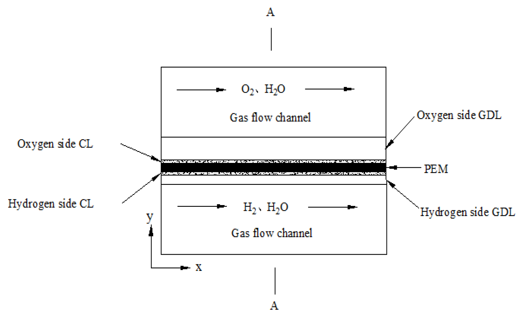
2. Model Description

2.1. Main Hypotheses of the Model
2.2. Governing Equations
2.2.1. Charge Balance

| Equations | Mode | |||
|---|---|---|---|---|
| FC Mode | WE Mode | |||
| Hydrogen Electrode | Oxygen Electrode | Hydrogen Electrode | Oxygen Electrode | |
| + | - | - | + | |
| - | + | + | - | |
2.2.2. Multicomponent Mass Transport
2.2.3. Gas Flow Equations
2.3. Initial and Boundary Conditions
- (1)
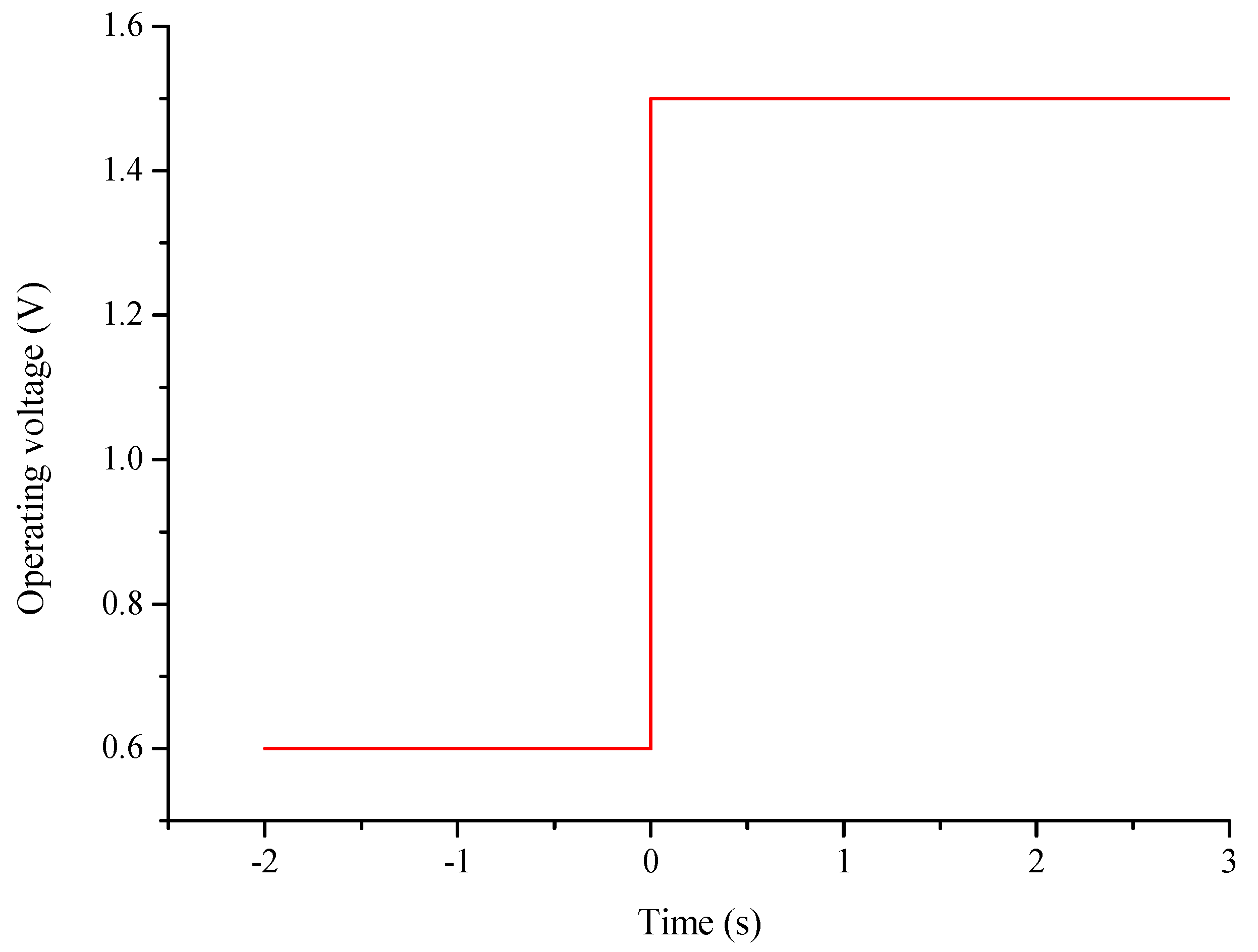
- For the GDL, CL at the H2 side and PEM: ,; for the GDL, CL at the O2 side: , (the operating voltage);
- (2)
- The initial values of the oxygen and hydrogen mass fractions are both 0.9.
3. Element Independence Test and Model Validation
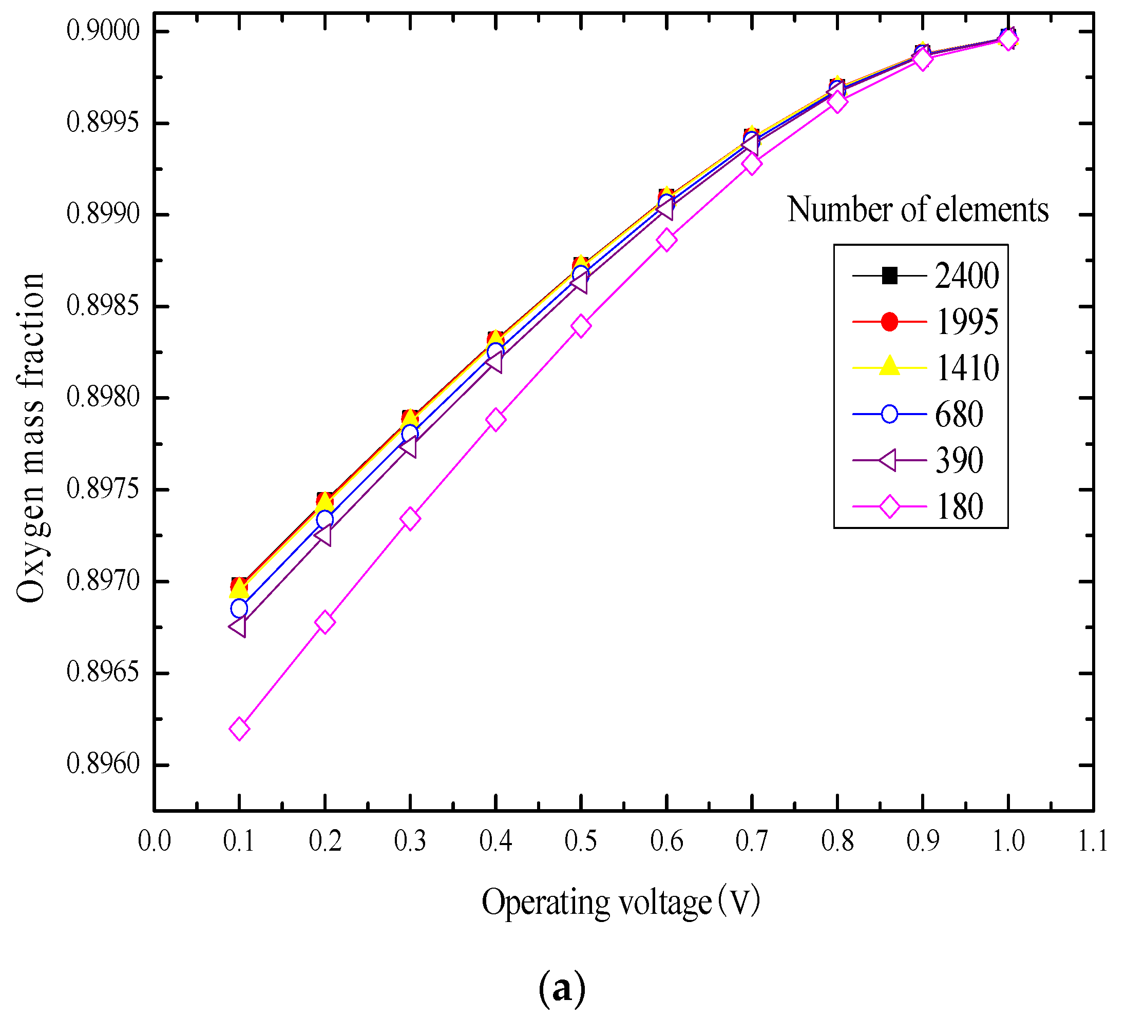
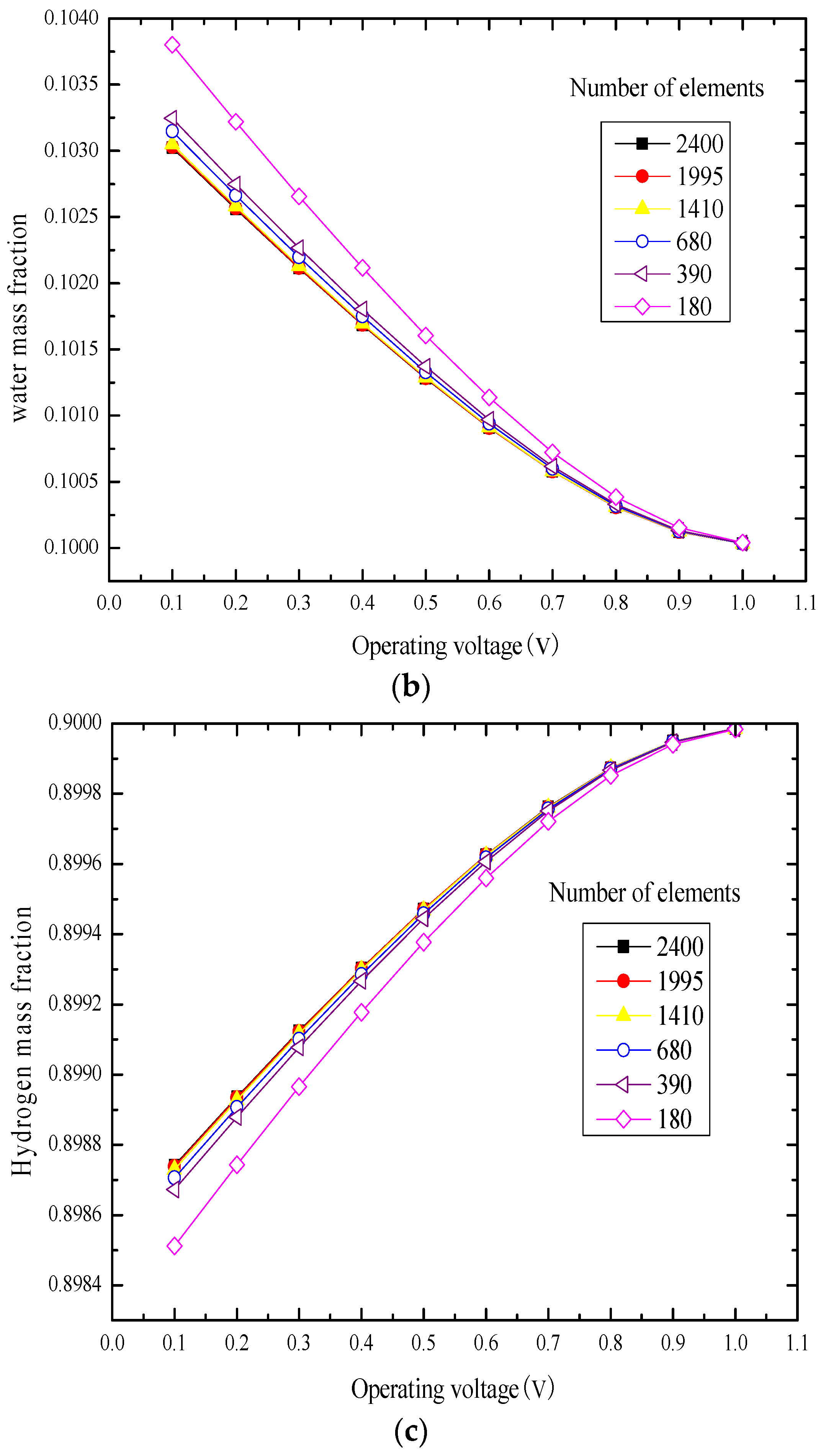
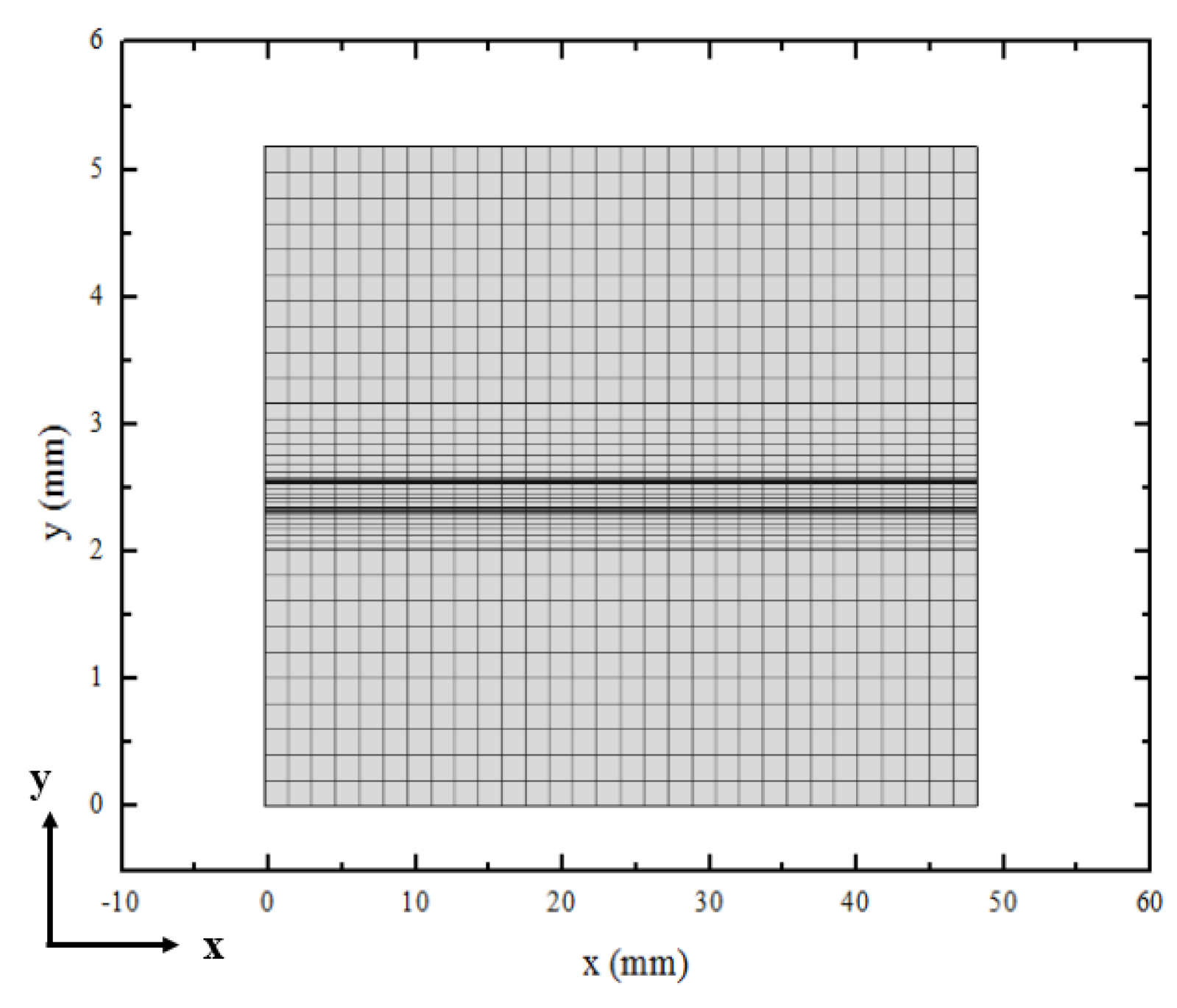
3.1. Element Independence Test


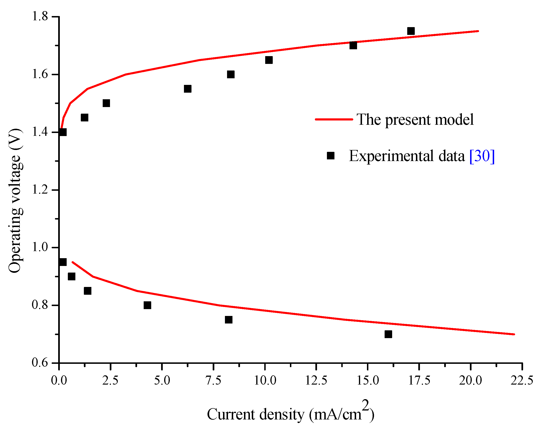
3.2. Model Validation

4. Results and Discussion

| Parameters | Value | References |
|---|---|---|
| Length of channel/mm | 48 | Assumed |
| Gas flow channel width/mm | 2 | Assumed |
| Oxygen electrode GDL thickness/mm | 0.6 | Assumed |
| CL thickness/mm | 0.028 | Assumed |
| Hydrogen electrode GDL thickness/mm | 0.3 | Assumed |
| Membrane thickness/mm | 0.178 | Assumed |
| H2 mass fraction | 0.9 | [32] |
| O2 mass fraction | 0.9 | [32] |
| O2/ H2 inlet pressure/Pa | 1.01 × 10⁵ | [32] |
| O2 inlet velocity/m·s−1 | 1.18 | [32] |
| H2 inlet velocity/m·s−1 | 0.53 | [32] |
| Oxygen/hydrogen electrode GDL permeability/m2 | 1.18 × 10⁻¹¹ | [32] |
| Membrane conductivity/S·m−1 | 1.4 | [32] |
| Oxygen/hydrogen electrode GDL electrical conductivity/S·m−1 | 1000 | [32] |
| H2 reference concentration/mol·m−3 | 56.4 | [33] |
| O2 reference concentration/mol·m−3 | 40.8 | [33] |
| Anodic transfer coefficient | 0.5 | [13] |
| Cathodic transfer coefficient | 0.5 | [13] |
| Operating temperature/K | 353 | [34] |
| Hydrogen electrode GDL porosity | 0.4 | [35] |
| Oxygen electrode GDL porosity | 0.5 | [36] |
| H2/H2O binary diffusion coefficient/m2·s−1 | 1.22 × 10⁻⁴ | Calculated |
| O2/H2O binary diffusion coefficient/m2·s−1 | 3.54 × 10⁻⁵ | Calculated |
| Oxygen/hydrogen electrode CL porosity | 0.25 | Assumed |
| Active specific surface area/m−1 | 1.4 × 10⁵ | Assumed |
| Reference temperature/K | 298.15 | Assumed |


5. Conclusions
- (1)
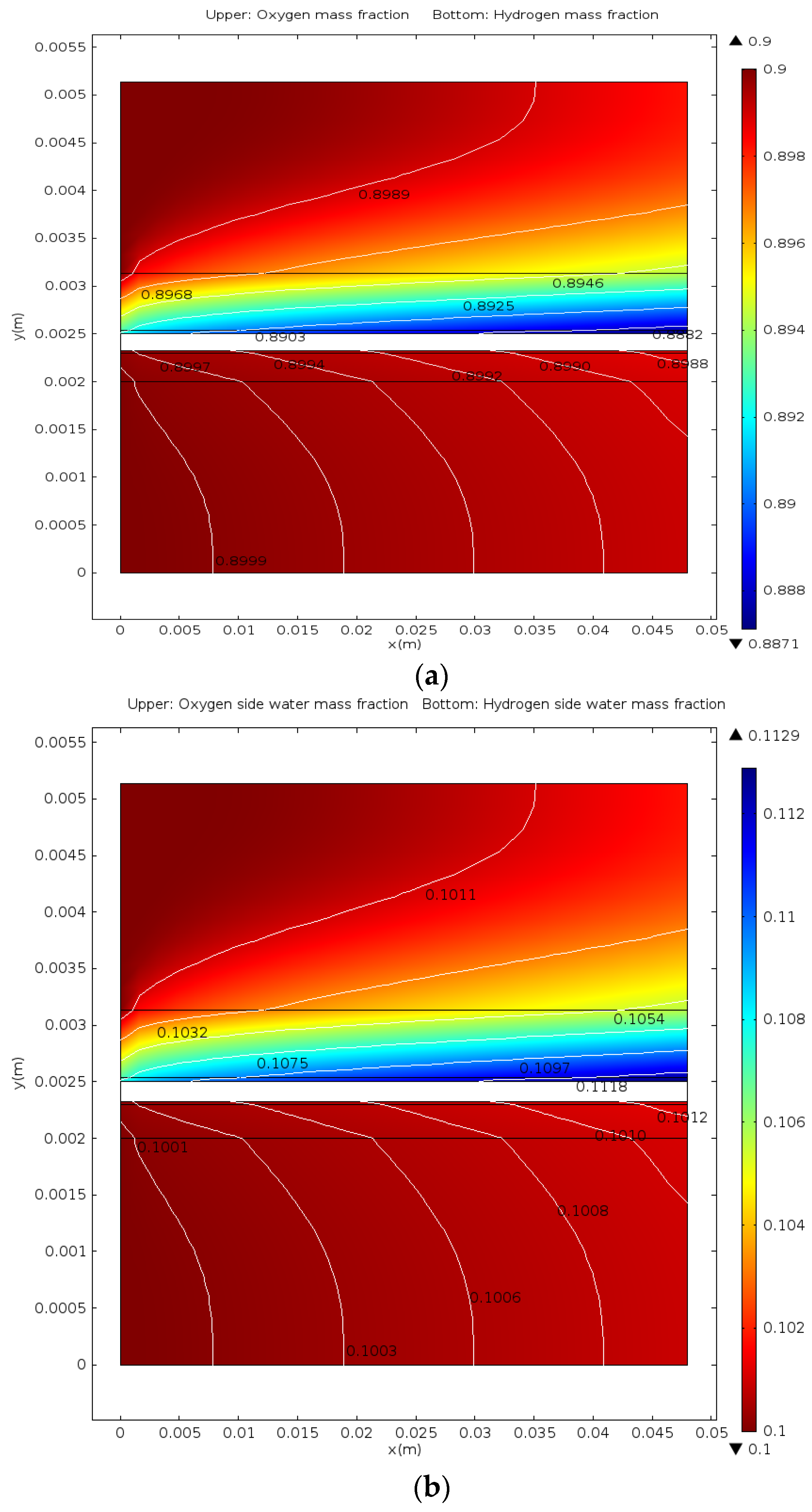
- The distributions of parameters, such as hydrogen, oxygen, water mass fractions, and electrolyte potential, respond to the operating voltage leap via a sudden change under operation mode switching.
- (2)
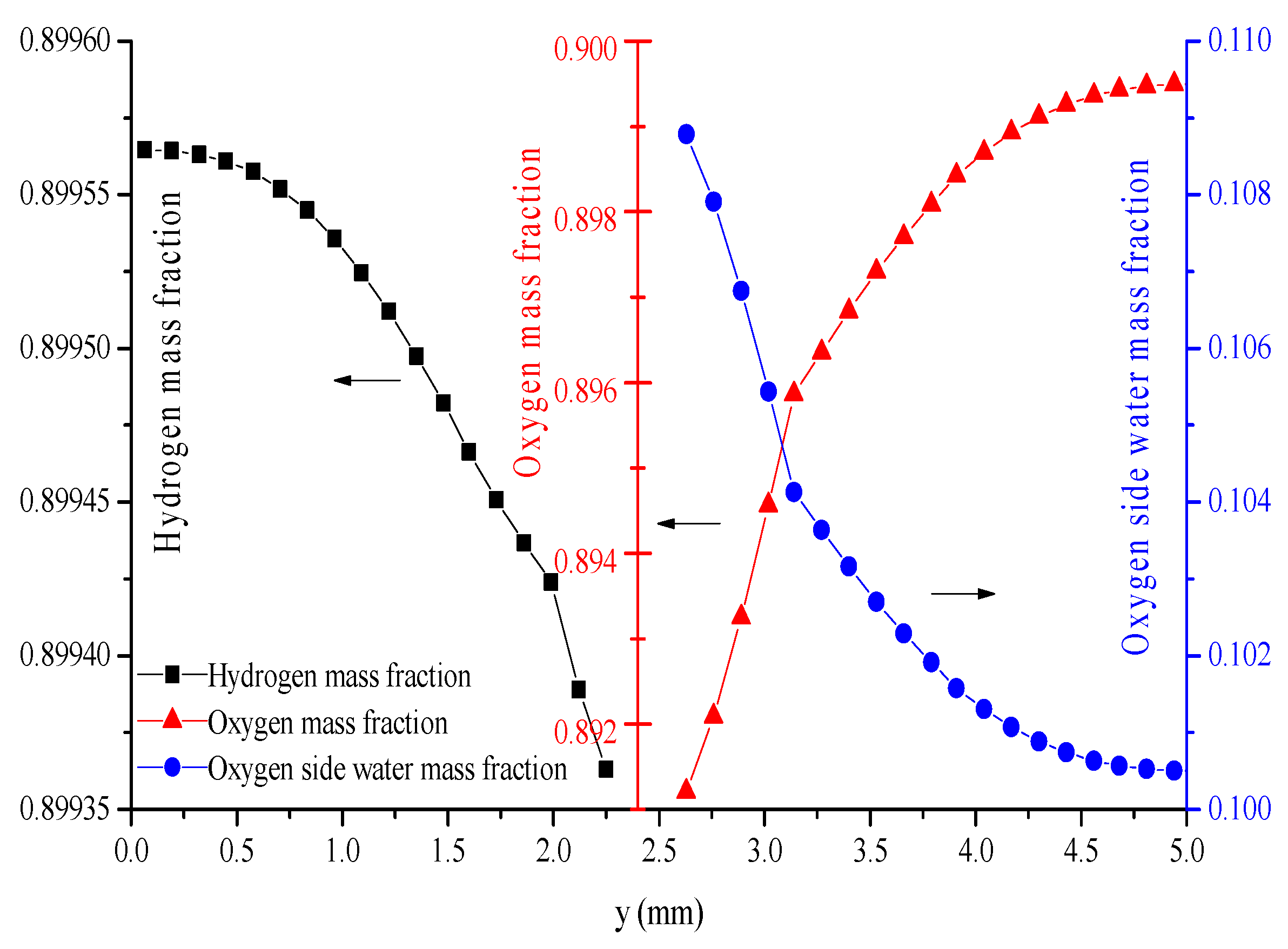
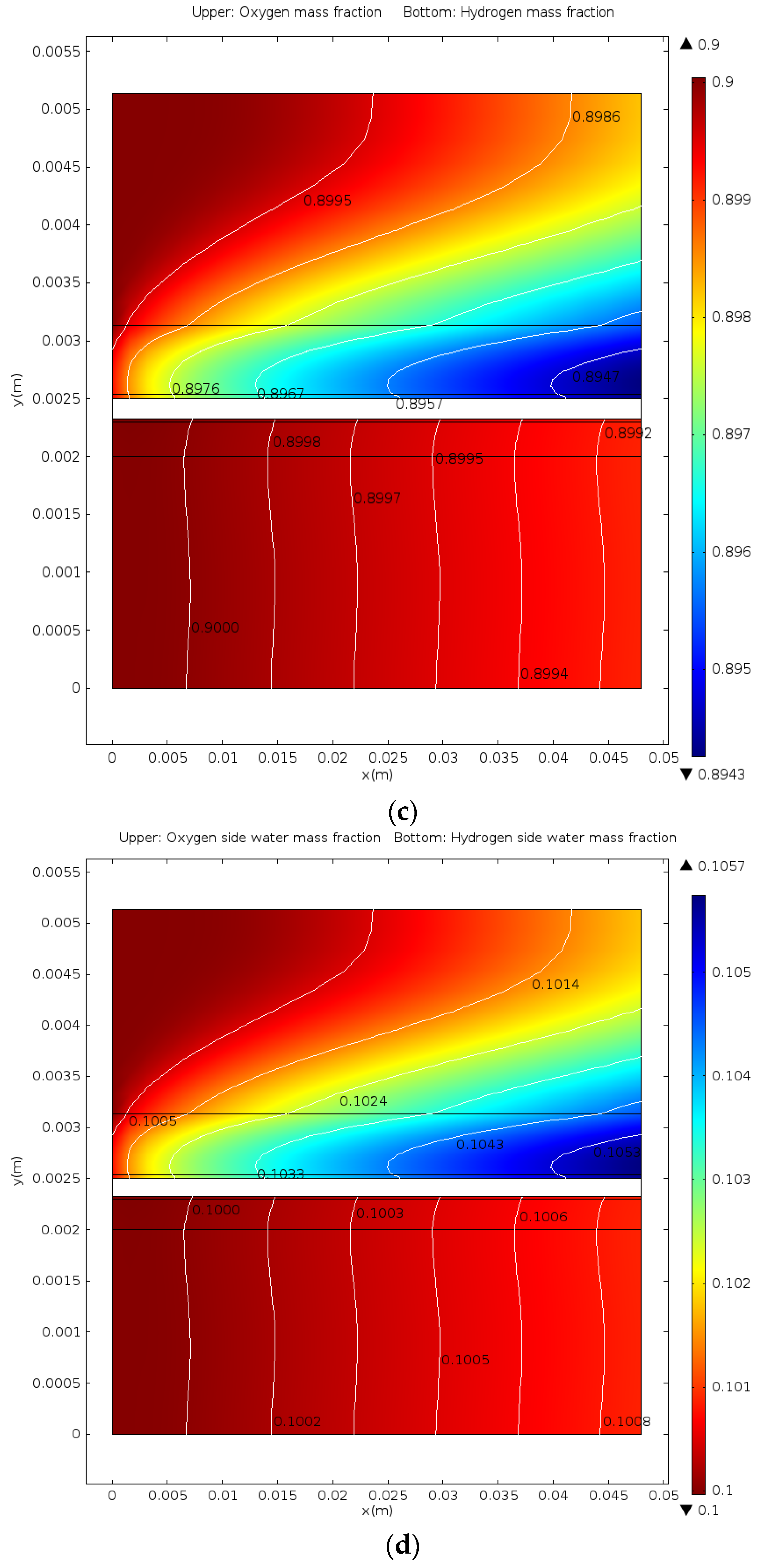
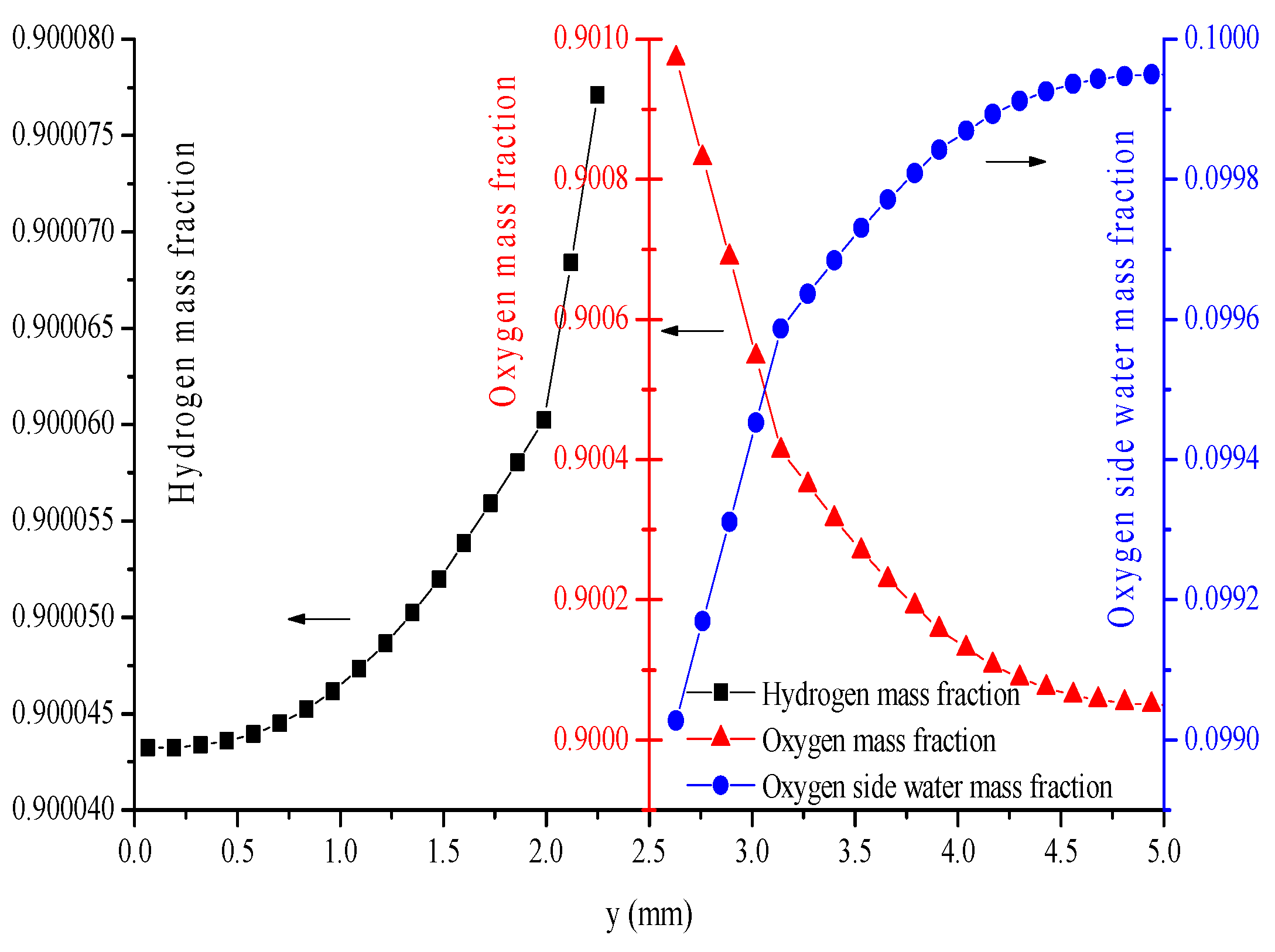
- The hydrogen mass fraction gradients are smaller than the oxygen mass fraction gradients for the same scale legend.
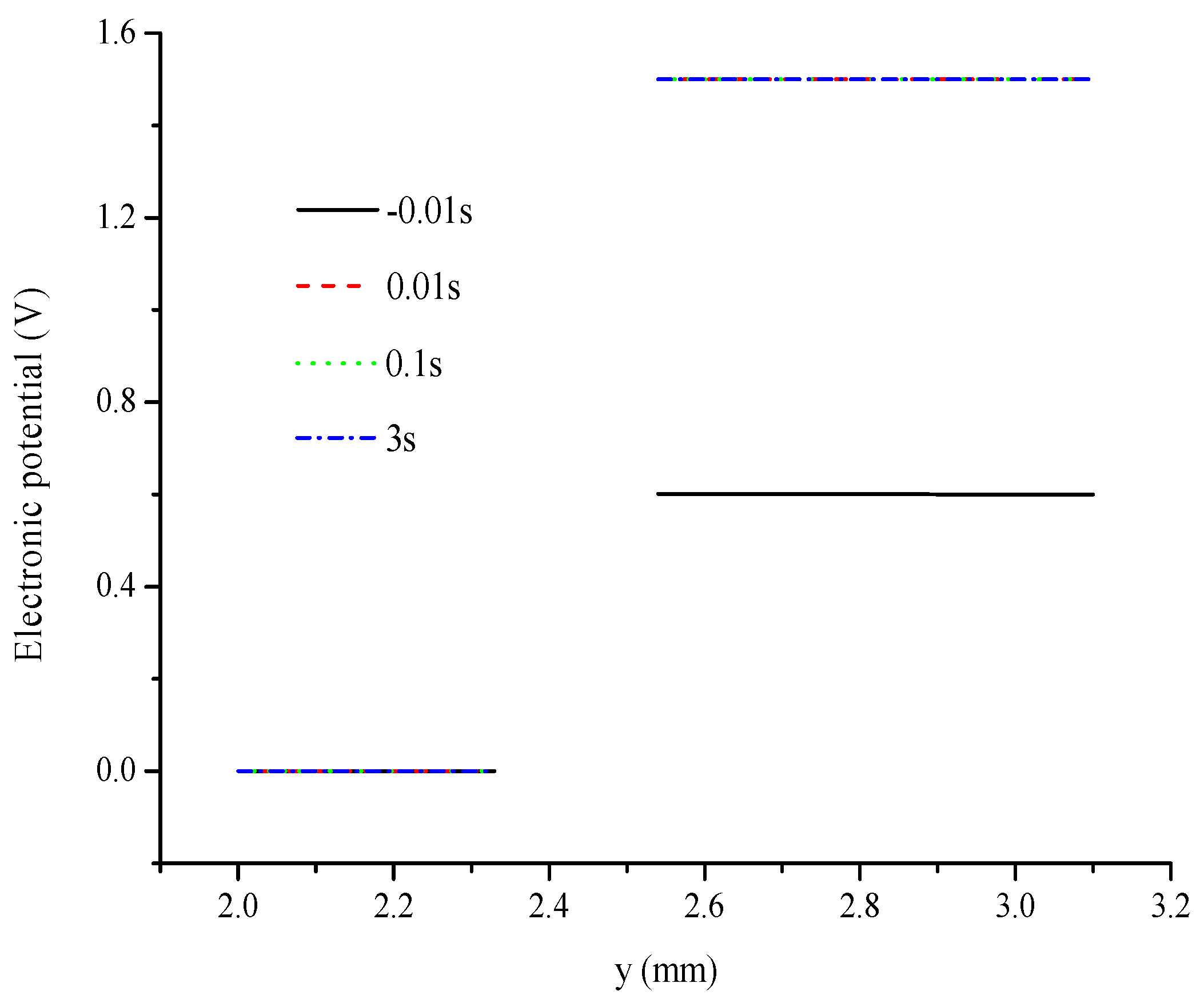
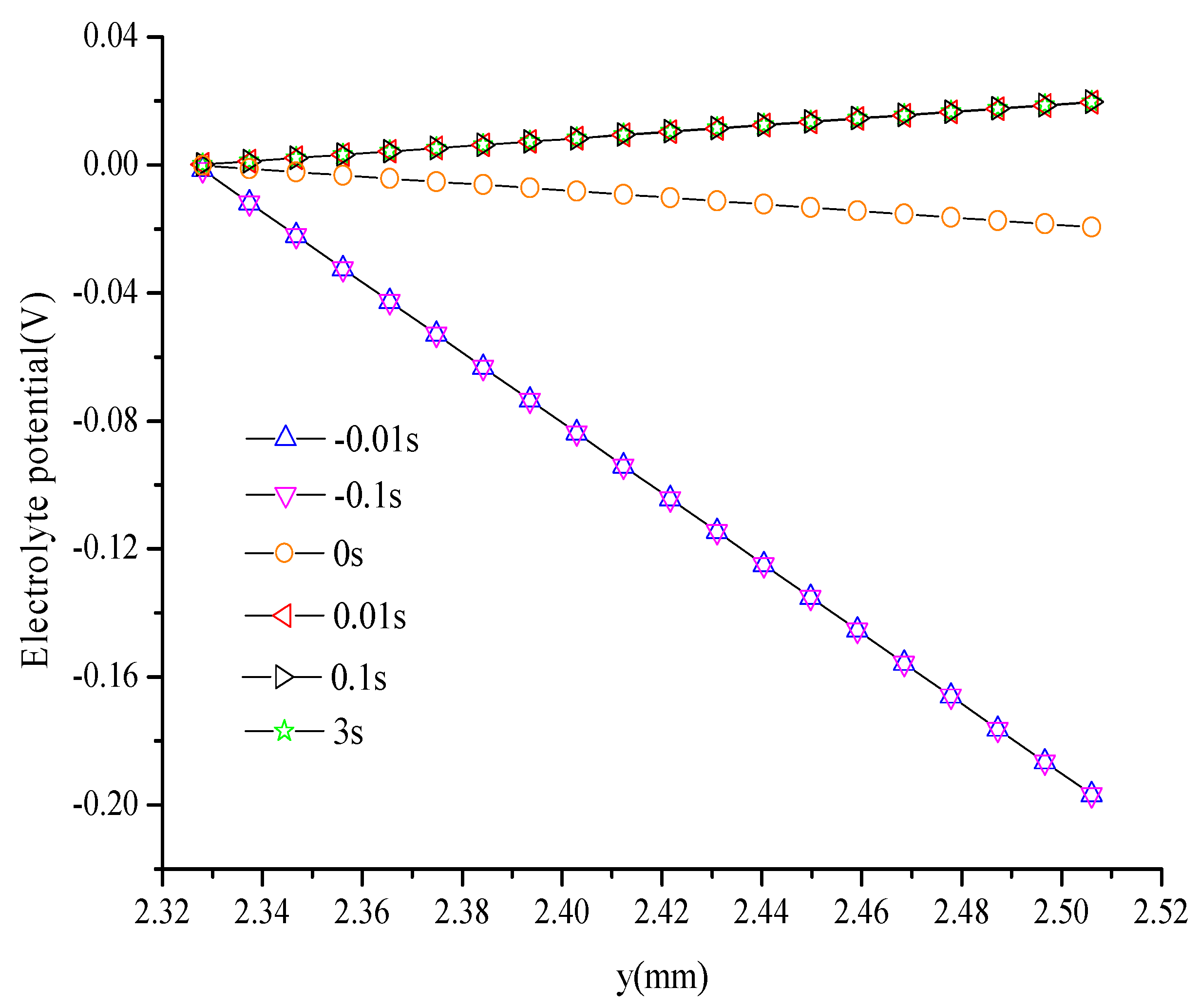
- (3)
- Electronic potential exhibits different trends compared with other parameters. At the hydrogen electrode, the electronic potential is maintained at zero in the switching mode. At the oxygen electrode, the electronic potential is maintained at approximately 0.6 V in the FC mode and is switched to approximately 1.5 V in the WE mode. The electrolyte potential increases linearly from the oxygen/hydrogen electrode to the hydrogen/oxygen electrode in the FC/WE mode.
- (4)
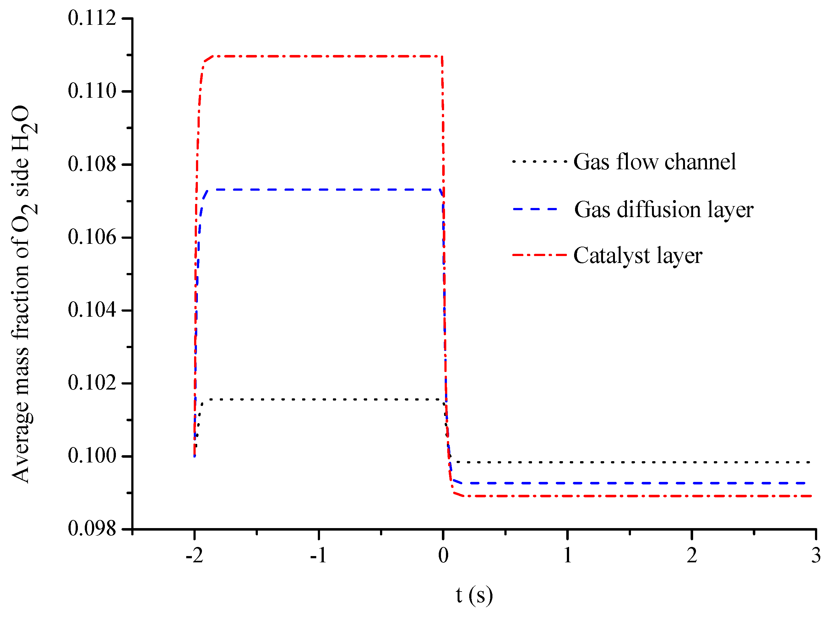
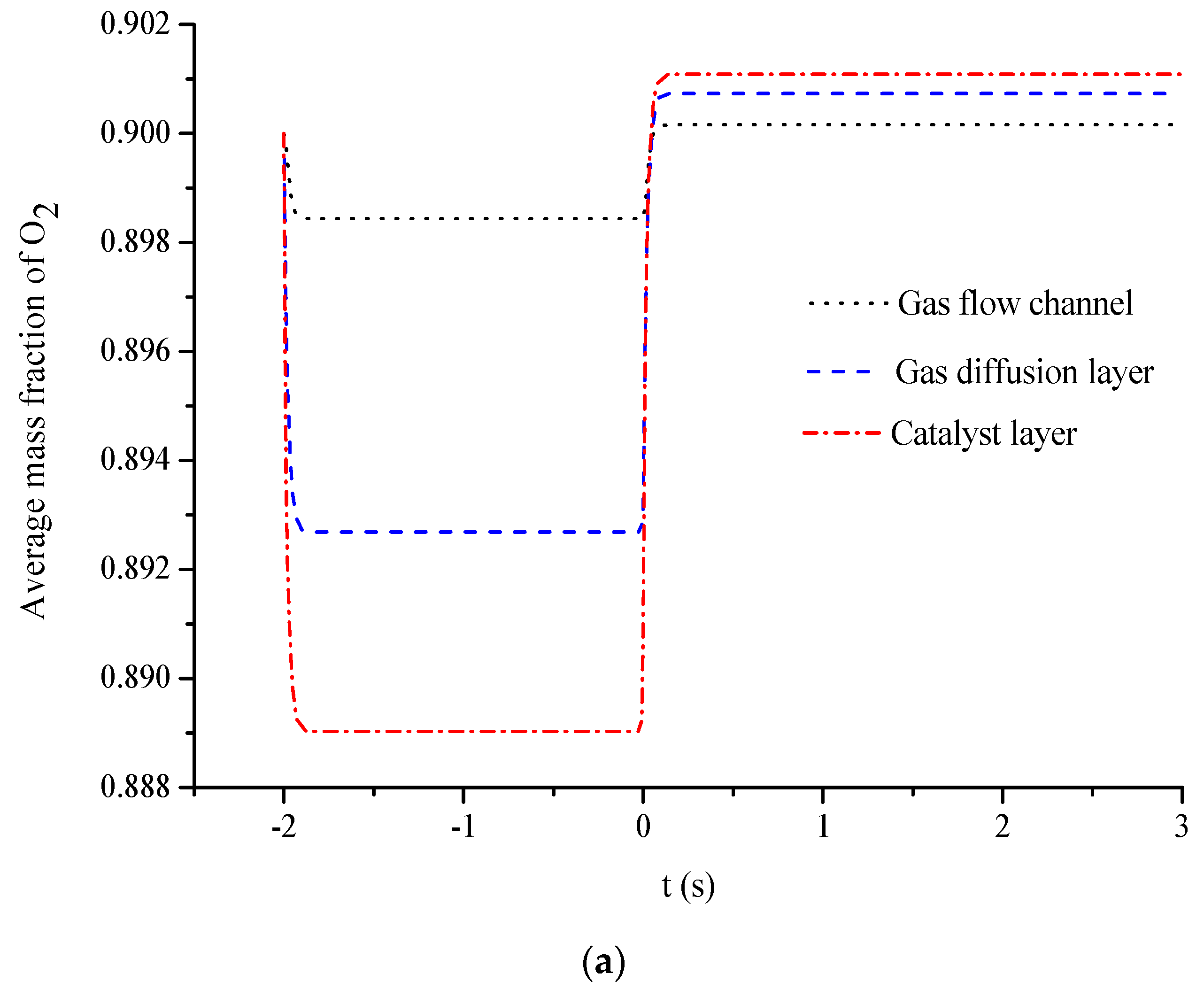
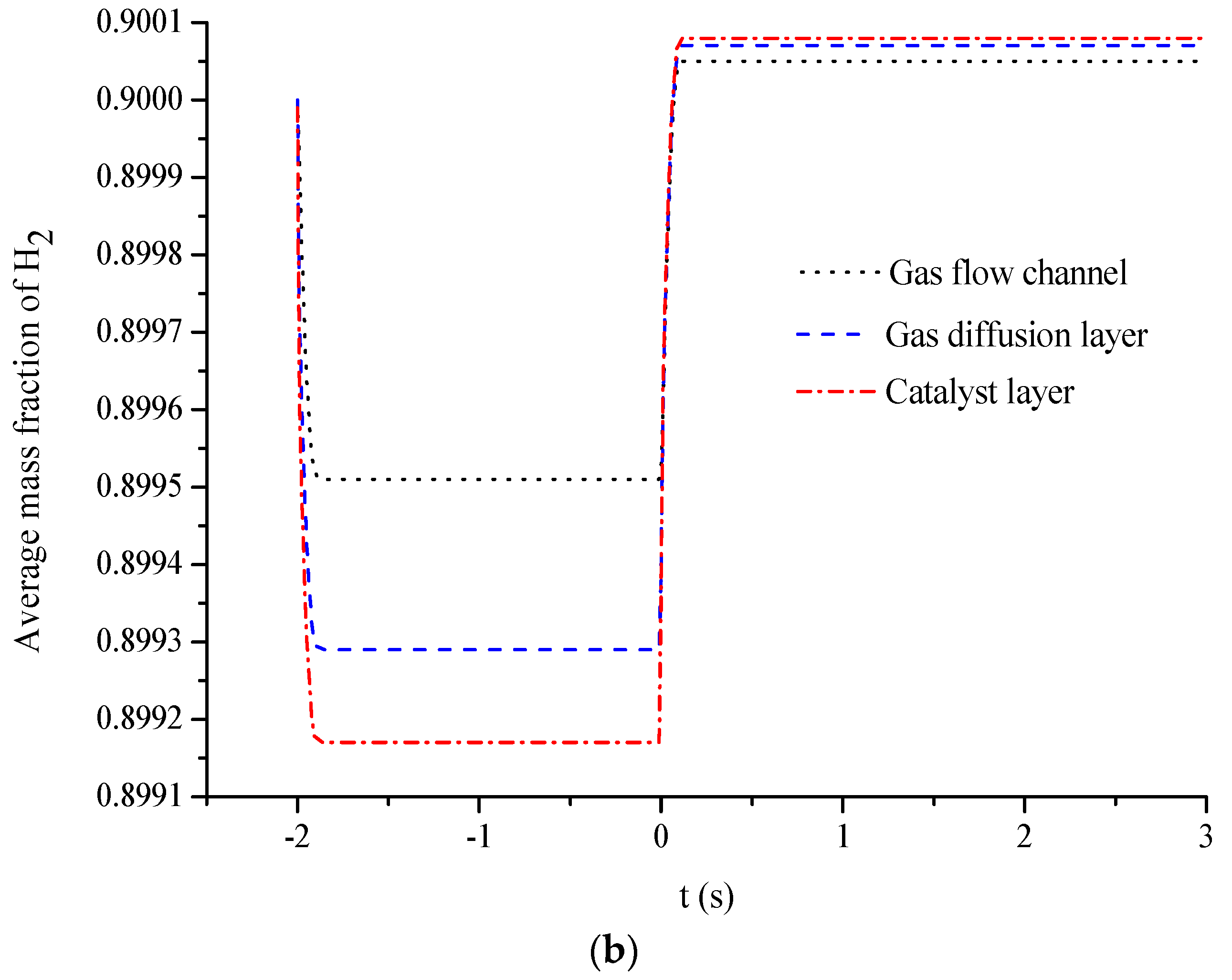
- The average mass fractions of the reactants (O2 and H2) and product (H2O) exhibit evident differences between each layer in the steady state of the FC mode. By contrast, the average mass fractions of the reactant (H2O) and products (O2 and H2) exhibit only a slight difference between each layer in the steady state of the WE mode.
- (5)
- The duration of the switch from the transient state to the steady state in either the FC mode or the WE mode is only approximately 0.2 s.
Acknowledgments
Author Contributions
Conflicts of Interest
Nomenclature
| local current density (mA·cm−2) | |
| exchange current density (mA·cm−2) | |
| F | Faraday’s constant (C·mol−1) |
| R | gas constant (J·mol−1·K−1) |
| equilibrium potential (V) | |
| reference equilibrium potential (V) | |
| T | temperature (K) |
| reference temperature (K) | |
| specific surface area (m−1) | |
| mass fraction of species i | |
| molar mass of species i (kg·mol−1) | |
| reaction source term for species i (kg·m−3·s) | |
| ik component of the multicomponent Fick diffusivity (m2·s−1) | |
| number of electrons in the reaction | |
| molar fraction of species k | |
| pressure (Pa) | |
| entrance length (m) | |
| mass flux relative to the mass average velocity (kg·m−2·s−1) | |
| diffusional driving force acting on species k (m−1) | |
| mass source term (kg·m−3) | |
| Greek letters | |
| conductivity of electron of ion (S·m−1) | |
| transfer coefficient | |
| over potential (V) | |
| electric potential (V) | |
| density of gases (kg·m−3) | |
| stoichiometric coefficient | |
| dynamic viscosity (Pa·s) | |
| porosity of medium | |
| permeability of medium (m2) | |
| Subscripts | |
| l | ionic |
| s | electronic |
| a | anodic |
| c | cathodic |
References
- Verma, A.; Basu, S. Feasibility study of a simple unitized regenerative fuel cell. J. Power Sources 2004, 135, 62–65. [Google Scholar] [CrossRef]
- Millet, P.; Ngameni, R.; Grigoriev, S.A. Scientific and engineering issues related to PEM technology: Water electrolysers, fuel cells and unitized regenerative systems. Int. J. Hydrog. Energy 2011, 36, 4156–4163. [Google Scholar] [CrossRef]
- Mitlitsky, F.; Myers, B.; Weisberg, A.H. Reversible (unitized) PEM fuel cell devices. Fuel Cells Bull. 1999, 11, 6–11. [Google Scholar] [CrossRef]
- Grigoriev, S.A.; Millet, P.; Porembsky, V.I. Development and preliminary testing of a unitized regenerative fuel cell based on PEM technology. Int. J. Hydrog. Energy 2011, 36, 4164–4168. [Google Scholar] [CrossRef]
- Applyby, A.P. Regenerative fuel cells for space applications. J. Power Sources 1988, 22, 377–385. [Google Scholar] [CrossRef]
- Markgraf, S.; Horenz, M.; Schmiel, T. Alkaline fuel cells running at elevated temperature for regenerative fuel cell system applications in spacecrafts. J. Power Sources 2012, 201, 236–242. [Google Scholar] [CrossRef]
- Yoshitsugu, S. A 100-W class regenerative fuel cell system for lunar and planetary missions. J. Power Sources 2011, 196, 9076–9080. [Google Scholar]
- Guarnieri, M.; Alotto, P.; Moro, F. Modeling the performance of hydrogen-oxygen unitized regenerative proton exchange membrane fuel cells for energy storage. J. Power Sources 2015, 297, 23–32. [Google Scholar] [CrossRef]
- Herrera, O.E.; Wilkinson, D.P.; Merida, W. Anode and cathode overpotentials and temperature profiles in a PEMFC. J. Power Sources 2012, 198, 132–142. [Google Scholar] [CrossRef]
- Zhan, Z.G.; Wang, C.; Fu, W.G. Visualization of water transport in a transparent PEMFC. Int. J. Hydrog. Energy 2012, 37, 1094–1105. [Google Scholar] [CrossRef]
- Nguyen, T.V.; White, R.E. A water and heat management model for proton-exchange-membrane fuel cells. J. Electrochem. Soc. 1993, 140, 2178–2186. [Google Scholar] [CrossRef]
- Ramousse, J.; Deseure, J.; Lottin, O. Modeling of heat, mass and charge transfer in a PEMFC single cell. J. Power Sources 2005, 145, 416–427. [Google Scholar] [CrossRef]
- Hu, G.L.; Fan, J.R. A three-dimensional, multicomponent, two-phase model for a proton exchange membrane fuel cell with straight channels. Energy Fuels 2006, 20, 738–747. [Google Scholar] [CrossRef]
- Singh, D.; Lu, D.M.; Djilali, N. A two-dimensional ananlysis of mass transport in proton exchange membrane fuel cells. Int. J. Eng. Sci. 1999, 37, 431–452. [Google Scholar] [CrossRef]
- Marangio, F.; Santarelli, M.; Cala, M. Theoretical model and experimental analysis of a high pressure PEM water electrolyser for hydrogen production. Int. J. Hydrog. Energy 2009, 34, 1143–1158. [Google Scholar] [CrossRef]
- Nie, J.H.; Chen, Y.T. Numerical modeling of three-dimensional two-phase gas-liquid flow in the flow field plate of a PEM electrolysis. Int. J. Hydrog. Energy 2010, 35, 3183–3197. [Google Scholar] [CrossRef]
- Carmo, M.; Fritz, D.L.; Mergel, J. A comprehensive review on PEM water electrolysis. Int. J. Hydrog. Energy 2013, 38, 4901–4934. [Google Scholar] [CrossRef]
- Grigoriev, S.A.; Kalinnikov, A.A.; Millet, P. Mathematical modeling of high-pressure PEM water electrolysis. J. Appl. Electrochem. 2010, 40, 921–932. [Google Scholar] [CrossRef]
- Jung, H.Y.; Huang, S.Y.; Popov, B.N. High-durability titanium bipolar plate modified by electrochemical deposition of platinum for unitized regenerative fuel cell(URFC). J. Power Sources 2010, 195, 1950–1956. [Google Scholar] [CrossRef]
- Chen, G.B.; Zhang, H.M.; Zhong, H.X. Gas diffusion layer with titanium carbide for a unitized regenerative fuel cell. Electrochim. Acta 2010, 55, 8801–8807. [Google Scholar] [CrossRef]
- Pai, Y.H.; Tseng, C.W. Preparation and characterization of bifunctional graphitized carbon-supported Pt composite electrode for unitized regenerative fuel cell. J. Power Sources 2012, 202, 28–34. [Google Scholar] [CrossRef]
- Huang, S.Y.; Ganesan, P.; Jung, H.Y. Development of supported bifunctional oxygen electrocatalysts and corrosion-resistant gas diffusion layer for unitized regenerative fuel cell applications. J. Power Sources 2012, 198, 23–29. [Google Scholar] [CrossRef]
- Lee, W.H.; Kim, H. Optimization of electrode structure to suppress electrochemical carbon corrosion of gas diffusion layer for unitized regenerative fuel cell. J. Electrochem. Soc. 2014, 161, 729–733. [Google Scholar] [CrossRef]
- Gabbasa, M.; Sopian, K.; Fudholi, A. A review of unitized regenerative fuel cell stack: Material, design and research achievements. Int. J. Hydrog. Energy 2014, 39, 17765–17778. [Google Scholar] [CrossRef]
- Doddathimmaiah, A.; Andrews, J. Theory, modeling and performance measurement of unitized regenerative fuel cells. Int. J. Hydrog. Energy 2009, 34, 8157–8170. [Google Scholar] [CrossRef]
- Hoberecht, M.A.; Robert, D.G. Use of excess solar array power by regenerative fuel cell energy storage systems in low earth orbit. In Proceedings of the IEEE Energy Conversion Engineering Conference, Honolulu, HI, USA, 27 July–1 August 1997.
- Jin, X.F.; Xue, X.J. Mathematical modeling analysis of regenerative solid oxide fuel cells in switching mode conditions. J. Power Sources 2010, 195, 6652–6658. [Google Scholar] [CrossRef]
- Raj, A.; Shamim, T. Investigation of the effect of multidimensionality in PEM fuel cells. Energy Convers. Manag. 2014, 86, 443–452. [Google Scholar] [CrossRef]
- Ju, H.; Wang, C.Y. Experimental Validation of a PEM fuel cell model by current distribution data. J. Electrochem. Soc. 2004, 151, A1954–A1960. [Google Scholar] [CrossRef]
- Dihrab, S.S.; Razali, A.M. Studies on a single cell unitized regenerative fuel cells. In Proceedings of the 9th ESEAS International Conference on System Science and Simulation In Engineering, Iwate, Japan, 4–6 October 2010.
- Rabih, S.; Rallieres, O.; Turpin, C.; Astier, S. Experimental Study of a PEM Reversible Fuel Cell. 2011. Available online: http://www.icrepq.com/icrepq-08/268-rabih.pdf (accessed on 17 July 2015).
- Doubek, G.; Robalinho, E.; Cunha, E.F. Application of CFD techniques in the modeling and simulation of PBI PEMFC. Fuel Cells 2011, 11, 764–774. [Google Scholar] [CrossRef]
- Sehribani, U. Mathematical and Computational Modeling of Polymer Exchange Membrane Fuel Cells. Master’s Thesis, University of Nevada, Reno, NV, USA, August 2012. [Google Scholar]
- Hsuen, H.K.; Yin, K.M. Performance equations of proton exchange membrane fuel cells with feeds of varying degree of humidification. Electrochim. Acta 2012, 62, 447–460. [Google Scholar] [CrossRef]
- Ni, M. Computational fluid dynamics modeling of a solid oxide electrolyzer cell for hydrogen production. Int. J. Hydrog. Energy 2009, 34, 7795–7806. [Google Scholar] [CrossRef]
- Khazaee, I. Experimental investigation and numerical comparison of the performance of a proton exchange membrane fuel cell at different channel geometry. Heat Mass Transf. 2015, 51, 1177–1187. [Google Scholar] [CrossRef]
© 2016 by the authors; licensee MDPI, Basel, Switzerland. This article is an open access article distributed under the terms and conditions of the Creative Commons by Attribution (CC-BY) license (http://creativecommons.org/licenses/by/4.0/).
Share and Cite
Wang, L.; Guo, H.; Ye, F.; Ma, C. Two-Dimensional Simulation of Mass Transfer in Unitized Regenerative Fuel Cells under Operation Mode Switching. Energies 2016, 9, 47. https://doi.org/10.3390/en9010047
Wang L, Guo H, Ye F, Ma C. Two-Dimensional Simulation of Mass Transfer in Unitized Regenerative Fuel Cells under Operation Mode Switching. Energies. 2016; 9(1):47. https://doi.org/10.3390/en9010047
Chicago/Turabian StyleWang, Lulu, Hang Guo, Fang Ye, and Chongfang Ma. 2016. "Two-Dimensional Simulation of Mass Transfer in Unitized Regenerative Fuel Cells under Operation Mode Switching" Energies 9, no. 1: 47. https://doi.org/10.3390/en9010047
APA StyleWang, L., Guo, H., Ye, F., & Ma, C. (2016). Two-Dimensional Simulation of Mass Transfer in Unitized Regenerative Fuel Cells under Operation Mode Switching. Energies, 9(1), 47. https://doi.org/10.3390/en9010047