Methods for Global Survey of Natural Gas Flaring from Visible Infrared Imaging Radiometer Suite Data

Abstract

A set of methods are presented for the global survey of natural gas flaring using data collected by the National Aeronautics and Space Administration/National Oceanic and Atmospheric Administration NASA/NOAA Visible Infrared Imaging Radiometer Suite (VIIRS). The accuracy of the flared gas volume estimates is rated at ±9.5%. VIIRS is particularly well suited for detecting and measuring the radiant emissions from gas flares through the collection of shortwave and near-infrared data at night, recording the peak radiant emissions from flares. In 2012, a total of 7467 individual flare sites were identified. The total flared gas volume is estimated at 143 (±13.6) billion cubic meters (BCM), corresponding to 3.5% of global production. While the USA has the largest number of flares, Russia leads in terms of flared gas volume. Ninety percent of the flared gas volume was found in upstream production areas, 8% at refineries and 2% at liquified natural gas (LNG) terminals. The results confirm that the bulk of natural gas flaring occurs in upstream production areas. VIIRS data can provide site-specific tracking of natural gas flaring for use in evaluating efforts to reduce and eliminate routine flaring.

1. Introduction

Flaring is widely used to dispose of natural gas produced at oil and gas facilities that lack sufficient infrastructure to capture all of the gas that is produced (Figure 1). The term “associated gas” refers to natural gas that emerges when crude oil is brought to the Earth’s surface. This is the largest source of gas flaring. Smaller quantities of gas flaring occur at oil refineries and natural gas processing facilities. Because flaring is a waste disposal process, there is no systematic reporting of the flaring locations and flared gas volumes. Additionally, where flare volume data are reported, the data are typically self-reported by the flare operators, estimated from the difference between the natural gas volume produced and the quantity used or sold. It is therefore difficult to assess the reliability and accuracy of the reported data.

There are four distinct applications for site-specific estimates of flared gas volumes. First, there are carbon cycle analyses that rely on site-specific knowledge of the locations and magnitudes of greenhouse gas emissions to the atmosphere [1]. Second is the tracking of activities to reduce gas flaring [2]. Third is the identification of potentially attractive locations for gas utilization. Fourth is the calculation of the carbon intensity of fuels, such as the California Low Carbon Fuel Standard [3].

In this paper, we present a series of methods that produce site-specific estimation of flared gas volumes worldwide using data collected by the National Aeronautics and Space Administration/National Oceanic and Atmospheric Administration NASA/NOAA Visible Infrared Imaging Radiometer Suite (VIIRS). Using data collected in 2012, we conducted a global survey of gas flaring sites and separated these into upstream (production sites) and downstream refineries and liquefied natural gas (LNG) terminals. We developed a calibration for estimating flared gas volumes and applied this to the individual sites. The results have been aggregated to the national level, with tallies of the number of flaring sites and estimates for the total flared gas volume in 2012.

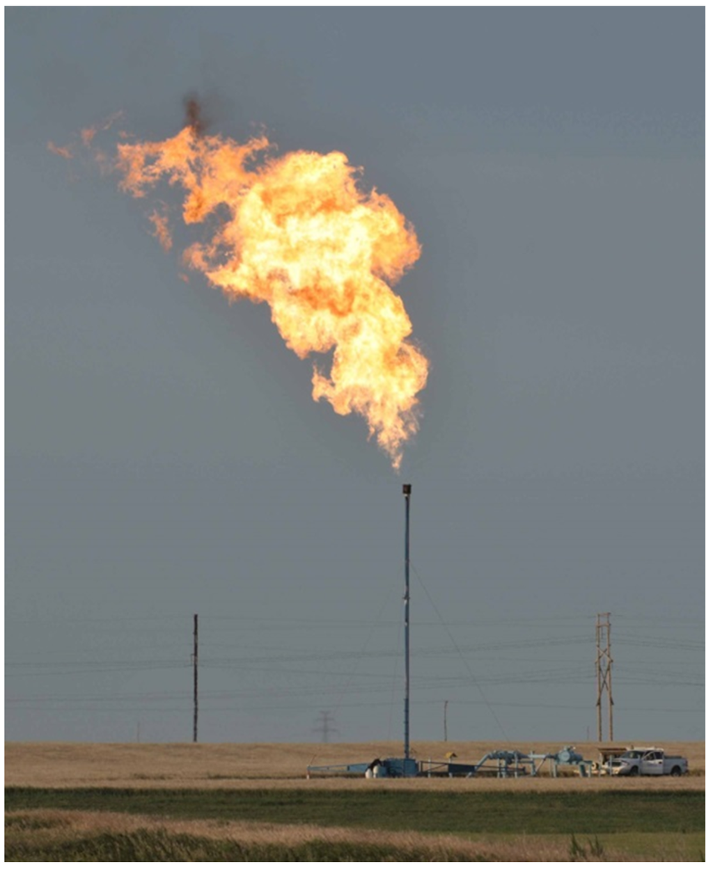
Figure 1. Large quantities of radiant energy are produced by gas flares.

Figure 1. Large quantities of radiant energy are produced by gas flares.

2. Satellite Observation of Gas Flares

Because of the lack of systematic reporting from flare operators and the remote nature of many flare locations, satellite sensors are an attractive option for global monitoring of gas flares. However, none of the existing sensors have been designed specifically for the detection and monitoring of gas flares. Systems that collect at high spatial resolution are not well suited to collect global data on large numbers of flare sites, lacking a repeat cycle suitable for cloud clearing and capturing the variability in flaring activity. In addition, the high spatial resolution sensors need to be tasked to collect data at specific sites, and the data are sold commercially, significantly raising the cost and complexity of any potential effort for global gas flaring monitoring. For global monitoring of gas flares, the option to analyze data from moderate spatial resolution (~1 km²) polar orbiting sensors has considerable merit. Here, the data are free and the coverage is global every 24 h. The challenge with this style of data is that flares are subpixel sources requiring specialized analysis to identify flares and to extract the flaring radiant emissions.

There have been several published studies describing gas flaring detection using satellite systems. NASA’s moderate-resolution imaging spectroradiometer (MODIS) data were used to inventory gas flares with the 4 µm spectral band and to estimate flared gas volumes in Nigeria [4]. Nighttime shortwave infrared (SWIR) data from advanced along track scanning radiometer (AATSR) have been used to map gas flares globally based on the temporal persistence of gas flares [5]. A survey of gas flaring sites was developed for a portion of Canada using daytime data collected by Landsat 8 [6].

To date, the most extensive time series of global gas flaring, with national estimates of flared gas volumes, comes from low light imaging nighttime data acquired by the Operational Linescan System (OLS) operated by the U.S. Air Force Defense Meteorological Satellite Program (DMSP) [7]. Gas flares were identified visually in DMSP data because the sensor detects electric lights from cities and towns, as well as gas flares. Estimation of gas flaring volumes using DMSP data ended in 2012 due to orbit degradation, resulting in solar contamination.

This study was conducted using VIIRS data on the Suomi National Polar Partnership (SNPP) satellite, launched in 2011. The VIIRS is operated in an unusual way that offers a substantial advantage for the observation of gas flaring. At night, the VIIRS continues to record data in three near- to short-wave infrared channels designed for daytime imaging (Figure 2). At night, the only features detected in these channels are combustion sources [8]. The SWIR channel, at 1.6 µm, is at the wavelength region where peak radiant emissions from gas flares occur. The 4 µm channel, widely used in fire detection [9], only detects large flares due to the fact that it falls on the trailing edge of gas flare radiant emissions and observes a mixture of flare plus background radiant emissions. Typically, the flare radiant emissions in the 4 µm channel are about a third of the emissions at 1.6 µm. This has a dramatic effect, limiting the detection of smaller flares in standard satellite fire products based on channels set at the 4 µm wavelength.

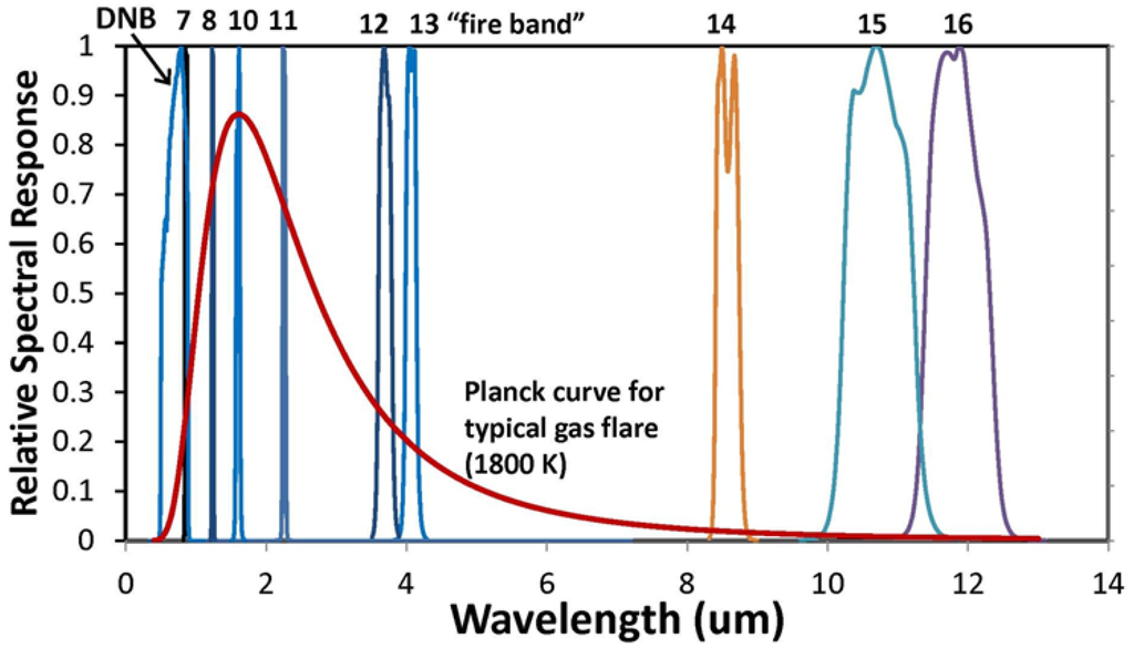
Figure 2. Relative spectral response of visible infrared imaging radiometer suite (VIIRS) bands and the Planck curve of typical gas flares at 1800 K. Day night band: DNB.

Figure 2. Relative spectral response of visible infrared imaging radiometer suite (VIIRS) bands and the Planck curve of typical gas flares at 1800 K. Day night band: DNB.

By detecting flare radiances in multiple spectral bands, it is possible to model Planck curves for gas flares. The temperature of the hot source is calculated using Wien’s displacement law:

T = b/ʎ_max

(1)

where T is temperature in kelvin (K), b is Wien’s displacement constant = 2897.8 K*μm and ʎ_max is the wavelength of peak radiant emissions.

The gas flares appear as graybodies because they are sub-pixel sources. The emission scaling factor (ε) is defined as the ratio between the observed radiances and the radiances for an object at that temperature filling the entire field of view. The source area (S) is calculated by multiplying ε by the size of the pixel footprint. Radiant heat (RH) is calculated using the Stefan–Boltzmann law:

RH = σT⁴S

(2)

where RH = radiant heat in megawatts (MW), σ = the Stefan–Boltzmann constant, T is temperature in K and S = source area in square meters.

Figure 2 shows spectral bands collected by VIIRS at night. Bands M7-10 are daytime spectral bands that continue to be collected at night, enabling unambiguous detection of combustion sources at 0.87 µm, 1.24 µm and 1.6 µm. Nighttime collection with the M11 band at 2.2 µm, which will improve detection and quantification of gas flares, has been approved for VIIRS and is expected to commence in 2016. The solid red line is the Planck curve for an 1800 K object, typical of a gas flare. The M10 spectral band records the peak radiant emissions from the typical gas flare.

3. Methods

3.1. Visible Infrared Imaging Radiometer Suite Nightfire Processing

The VIIRS Nightfire (VNF) algorithm [8] was applied to all of the usable nighttime VIIRS data from 2012. The usable record started 1 March 2012 and ran to the end of December, 2012. This processing included the detection of subpixel hot sources in five spectral bands (M7, M8, M10, M12 and M13). Redundant “bow-tie” pixels found along the outer portions of the swath were marked for exclusion in the output. The location (latitude, longitude) of the hot pixels, spectral radiances, satellite zenith angle and cloud state were recorded in the output. While all detected pixels were recorded in the output, local maxima were marked. As cloud cover falsely provides a ‘no flaring’ signal, pixel cloud states were extracted from VIIRS using a cloud mask (VCM) [10], so that these non-detections can be ignored. While the VCM generally successfully identifies cloud cover, it sometime identifies gas flares as clouds due to spectral confusion in the mid-wave infrared. To address this, VNF removes isolated patches of cloud where these coincide with M10 detections.

Planck curve fitting was applied to the detected pixels. Pixels with detection in M12 and M13 were processed with dual Planck curve fitting, with one Planck curve for the background and one for the hot source. From the Planck curve fits, temperature (K) and source area (m²) were calculated. A single hot source Planck curve fit is developed for pixels that lack detection in the M12 and M13 spectral bands.

Planck curve fitting cannot be performed on the pixels with detection in only a single spectral band. This is a common occurrence for small gas flares detected only in the M10 spectral band. The M10-only pixel detections were treated using a different set of processing steps for incorporation in the flared gas estimates (Section 3.5).

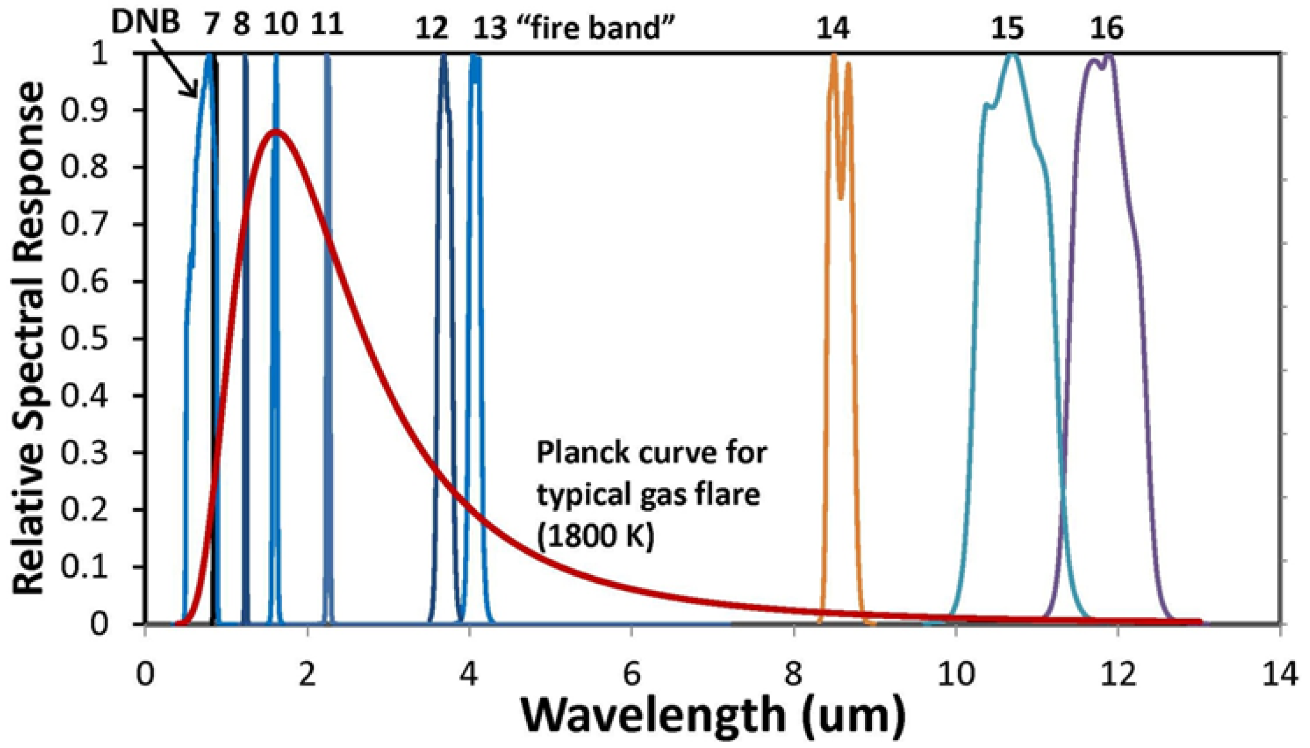
Examination of the results on a temperature versus source area basis reveals that there were two primary data clusters (Figure 3). There is a low temperature detection set, peaking in the 800–1200 K range, dominated by biomass burning. The high temperature set (above 1450 K) is dominated by gas flares, with peak numbers of flares in the 1700–1800 K range.

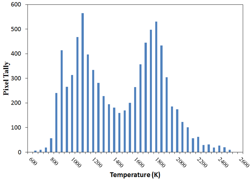
Figure 3. Temperature histogram for a single day of VIIRS Nightfire (VNF) data. The distribution is bimodal, with the majority of gas flares falling in the range from 1500 K to 2000 K. Biomass burning, industrial sites and volcanoes have temperatures in the 600–1300 K range. The range from 1300 K to 1500 K is a crossover zone between gas flares and biomass burning.

Figure 3. Temperature histogram for a single day of VIIRS Nightfire (VNF) data. The distribution is bimodal, with the majority of gas flares falling in the range from 1500 K to 2000 K. Biomass burning, industrial sites and volcanoes have temperatures in the 600–1300 K range. The range from 1300 K to 1500 K is a crossover zone between gas flares and biomass burning.

3.2. Analyzing Atmospheric Effects

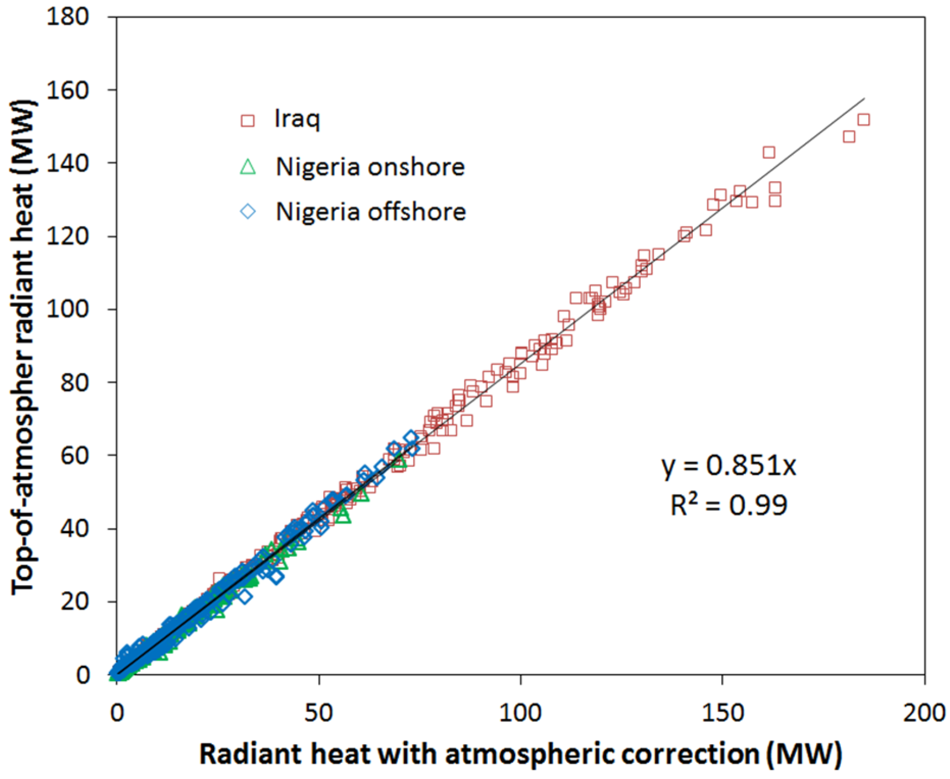
The VIIRS measures top-of-atmosphere (TOA) radiances. In some spectral bands, there can be substantial losses in radiance from the Earth’s surface to the TOA from atmospheric absorption and scatter. A study was conducted to analyze the effects of atmospheric variations on the VNF data. The study was based on a flare in Iraq (dry atmosphere) and two flares in Nigeria (moist atmosphere, onshore and offshore). Data included in the analysis spanned from 1 March 2012 to 31 December 2014. The analysis included all available satellite zenith angles. An atmospheric correction was developed for each of the VIIRS observations using the MODerate Resolution Atmospheric TRANsmission (MODTRAN) model [11] parameterized by atmosphere temperature, pressure and water vapor profiles, as well as ground temperature derived from simultaneously-acquired advanced technology microwave sounder (ATMS) data and a surface elevation model. For each observation, RH (MW) was calculated with and without the atmospheric correction. It was found that there is a strongly coherent linear relationship between the TOA and atmospherically-corrected RH data (Figure 4). We attribute this to the fact that the M10 spectral band is in a clear atmospheric window. Based on these results, the study was conducted with the uncorrected TOA radiances.

Figure 4. Radiant heat (RH) for three gas flares, with and without atmospheric correction. Sites include onshore and offshore flares in Nigeria (moist atmosphere) and a flare in Iraq (dry atmosphere).

Figure 4. Radiant heat (RH) for three gas flares, with and without atmospheric correction. Sites include onshore and offshore flares in Nigeria (moist atmosphere) and a flare in Iraq (dry atmosphere).

3.3. Identifying Gas Flaring Sites

It is not possible to adequately separate gas flares from other hot sources based solely on temperature due to the overlap between high temperature biomass burning and low temperature gas flaring (Figure 3). To separate gas flares from fires, we use both temperature and persistence. To accomplish this, we built a global 15 arc second grid tallying the number of times an M10 detection occurred during the year. The vast majority of biomass burning events could be filtered out by excluding single and double detections. Manual editing was used to mask out the few remaining biomass burning events.

The remaining sites were divided into three classes based on their temperature records: (1) sites where the maximum temperature exceeded 1400 K; these were taken to be gas flares; (2) sites where temperatures never exceeded 1400 K; these are primarily industrial sites; and (3) sites with single band, M10 detections, where temperature could not be calculated. If the “no temperature” sites were within 10 kilometers of a gas flare, they were classed as potential gas flares and were subsequently resolved by visual inspection of satellite images. Finally, a water-shedding algorithm was used to separate conjoined gas flare features. A raster to vector algorithm was used to draw vectors defining the outlines of the individual gas flaring sites.

3.4. Building a Global Gas Flaring Database

A database was built to hold the time series of gas flaring detections from the individual VIIRS observations. The purpose of the database is to enable rapid extraction of the time series of VNF data for individual sites. The database has three tables, each with the spatial extensions. Table 1 is used to store all VNF detections as individual points. This includes the latitude and longitude of the pixel center, radiances from the individual spectral bands, view geometry and specification of local maxima within clusters of adjacent pixels. Table 2 stores boundaries for individual sites with the polygon geometry. The third table stores the date/time and the cloud state conditions for all satellite observations for the centroid points of the individual sites. A typical database query will select all of the VNF detections within an individual site polygon and fill the gaps when the flare was not detected with the dates and the cloud state observed at the site center.

3.5. Assigning Temperatures to M10-Only Flare Detections

Small flares often have detection only in a single band, M10, the location of peak radiant emissions for typical gas flares. In these cases, it is not possible to model a Planck curve to derive temperature and source area, and there is insufficient information therefore to calculate the RH with the Stefan–Boltzmann law. We develop two methods for assigning temperatures to M10-only gas flare detections. The first method is used in cases where the flare site had observations on other nights with Planck curve fits. In this method, the M10-only detections were assigned the average temperature for flare observations from the same site. The second method is used for cases where the flare site never has observations with Planck curve fits. In this case, a temperature is assigned from the nearest flare site having Planck curve fits. Using these methods for assigning temperatures, it was possible to calculate source areas and RH values for weak flare detections based on the M10 radiance.

3.6. Adjusting Flare Area Estimates for View Angle Differences

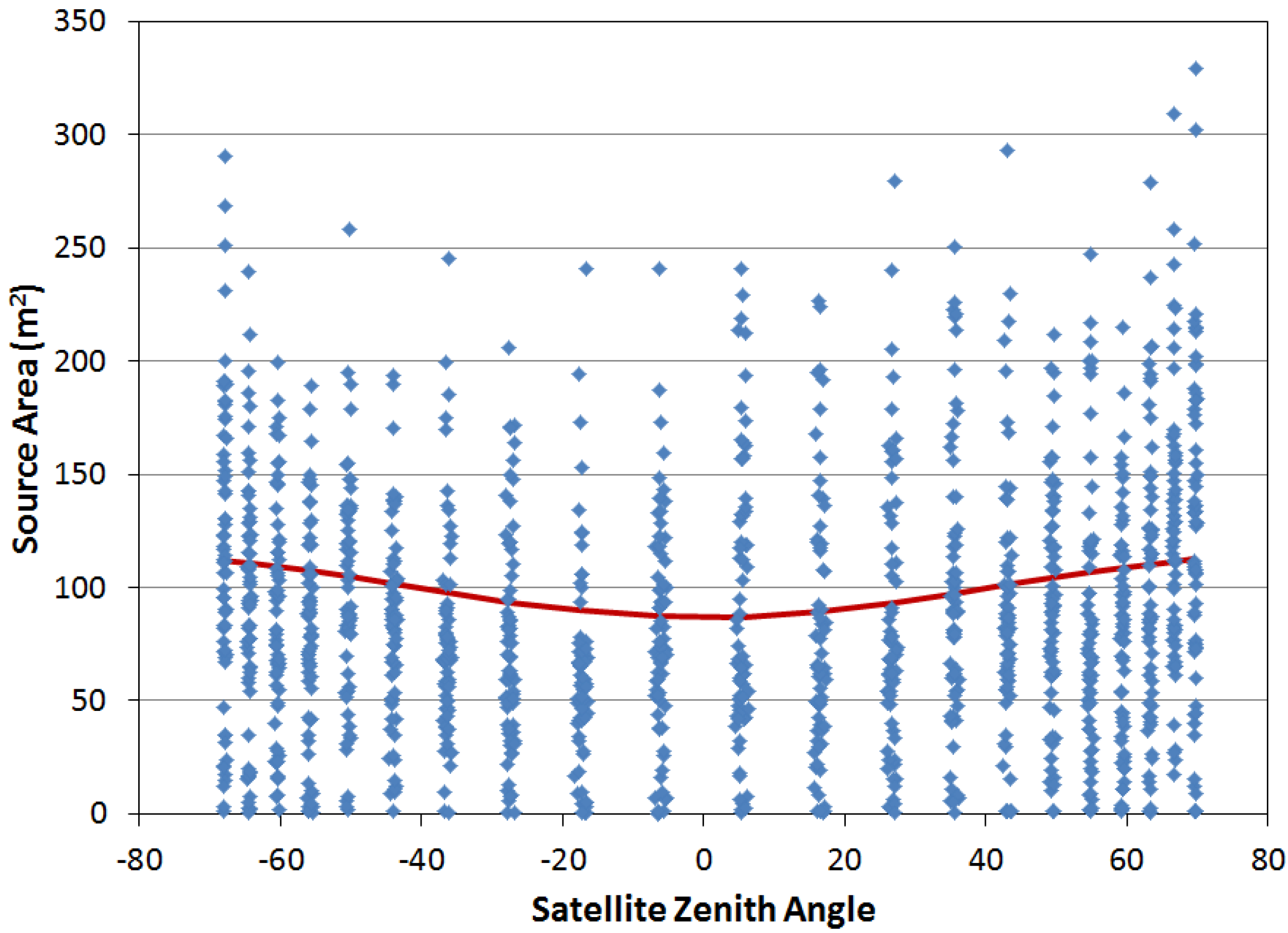
VIIRS observes the Earth at satellite zenith angles ranging from zero (nadir) to 70 degrees (edge of scan). In examining the observed signals from flares, we found that flares tend to have higher radiance when viewed at high satellite zenith angles. Our interpretation of this phenomena is that flares are typically taller than they are wide due to the buoyancy of the hot gas relative to the surrounding air (Figure 1). Thus, flare footprints appear larger when viewed from the side and smaller when viewed from straight above (the nadir view). The expression of this in VIIRS data is that the flares have higher radiance when viewed at an oblique angle when compared to the nadir, yet the temperature remains stable across all viewing angles. This results in larger source areas for flares when viewed at the edge-of-scan.

The three-dimensional shape of flares can be modeled as an ellipsoid, based on the apparent size of flares versus the satellite zenith angle (Figure 5). Using the approach developed by Jekrard [12], it is possible to derive the ellipticity or height (H) versus width (R) ratios of individual flares. For a vertically-standing flare, the footprint viewed by satellite from a zenith angle α will be:

$$S\left(\mathsf{\alpha },H,R\right)=\mathsf{\pi }R\sqrt{\left(H^2+R^2-\left(H^2-R^2\right)\cos 2\mathsf{\alpha }\right)/2}$$

(3)

Testing indicated that the calibration to flared gas volumes had a higher coefficient of determination (R²) if the source size was adjusted to the side view. For frequently-observed flares, it is generally possible to calculate the ellipticity, in which cases, the source sizes were adjusted to a horizontal side view or satellite zenith angle of 90 degrees. For flares with infrequent detection, we used the average ellipticity of 1.6.

Non-linear regression of Equation (3) to the set of average flare footprints S(α_i) from different satellite zenith angles α_i can estimate the flare shape H/R. Typical flares have ellipticities in the range of 1–4, with an average of 1.6.

Figure 5. Variation in flare area estimates as a function of satellite zenith angle. The red line is the best fit line based on an elliptical model of the flare shape.

Figure 5. Variation in flare area estimates as a function of satellite zenith angle. The red line is the best fit line based on an elliptical model of the flare shape.

3.7. Discrimination of Flare Types

Flare sites were divided into upstream (or production) sites, downstream processing sites and flares at LNG terminals. This was based on spatial databases [13] containing 658 refineries and 35 LNG terminals combined with visual inspection of high spatial resolution images available in Google Earth. The upstream sites include oil and natural gas production facilities. Downstream sites are primarily refineries, identified either from the database or based on the spatial extent of infrastructure and large numbers of circular storage tanks. In some cases, oil refineries are adjacent to LNG terminals, with each site having flares. In this case, the LNG section was identified based on the presence of LNG carrier loading infrastructure and LNG storage tanks.

3.8. Calibration to Estimate Gas Flaring Volumes

RH with units of MW, is calculated from temperature and source size using the Stefan–Boltzmann law (Equation (2)). Although the efficiency of gas combustion at the flare and variations in gas composition (gas heating value) somewhat affect the relationship between gas volume entering a flare and the RH emitted, there should be a reasonably consistent relationship between the reported flare volumes and the estimated RH. We attempted to develop a calibration for estimating flared gas volumes based on the monthly sum of RH estimates (normalized for cloud cover and the number of valid nighttime observations) versus reported flaring from individual sites in Nigeria, Texas and North Dakota. Over the limited range of data available, the calibration appeared linear. When applied globally, however, the linear calibration resulted in unrealistically high flared gas volumes for the largest ~100 flares out of the >7000 detected globally. This result implied that there is a non-linear relationship between RH and flared gas volumes, with RH growing in a logarithmic fashion relative to flared gas volume.

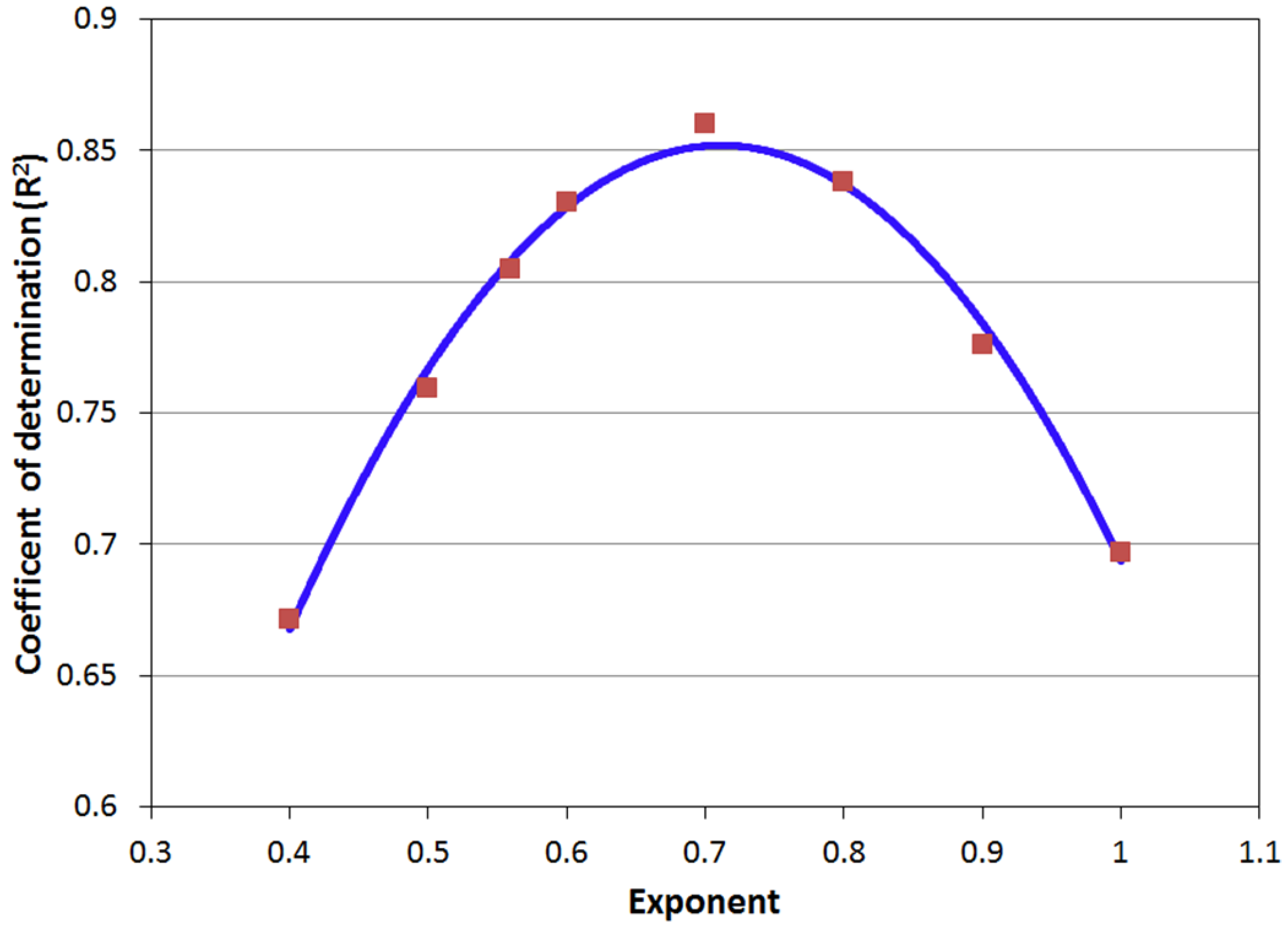
To address this issue, we developed a non-linear calibration using national-level reporting of upstream flaring (plus venting) for 47 countries provided by Cedigaz [14], plus state-level reporting for Texas and North Dakota. Non-linearity was introduced by applying an exponent to the source area in the calculation of a modified RH estimate, RH', for each flare. As part of the calibration process, the value of the exponent was tuned to achieve the highest possible R² coefficient of determination between reported flare volumes and RH' (Figure 6). As vented gas does not contribute to RH emissions, we assumed that the quantity of reported venting was negligible. This was reasonable, as gas venting is rare and generally not reported by oil field operators. For the calibration, annual RH' estimates from all of the upstream gas flaring sites within the national boundaries were summed, with normalization for cloud cover and the number of valid nighttime observations.

Cedigaz includes only flare volumes at oil fields in its reported data. In Russia, in particular, there is a substantial volume of flaring at non-associated gas and gas condensate fields, which is not included in the Cedigaz estimates. Indeed, the RH' for flaring in all of Russia is high relative to the Cedigaz reported number (Figure 7). To remedy this, the Russian flares were associated with vector maps of oil fields, natural gas fields and gas condensate fields, and only the RH' for flares related to oil fields were used for the calibration.

To determine the optimal exponent for modulating the source areas for estimating RH', source areas were modulated using exponents ranging from 0.4 to 1.0 and evaluating the coefficient of determination (R²) between RH' and the reported data. The highest R² occurred for an exponent of 0.7 (Figure 6).

Figure 6. The exponent applied to the flare source area was tuned to 0.7 to yield the highest coefficient of determination (R²).

Figure 6. The exponent applied to the flare source area was tuned to 0.7 to yield the highest coefficient of determination (R²).

The resulting calibration is shown in Figure 7. To estimate the slope in the linear equation BCM = slope × RH’ we use a standard linear regression through the origin. The confidence intervals for the total sum ± BCM are derived from the 95% confidence intervals of the regression slope multiplied by the total sum of the observed RH'.

Figure 7. Calibration for estimating flared gas volumes from VIIRS-derived RH based on Cedigaz reported data. The dashed red lines indicate the positions of the 95% confidence intervals for the billion cubic meter (BCM) prediction errors. Note that the Russian data used in the regression was filtered to remove flares in natural gas and gas condensate fields, since the flaring in these areas is not represented in the Cedigaz gas flaring estimates.

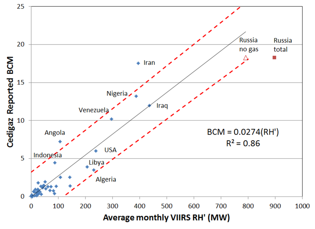
Figure 7. Calibration for estimating flared gas volumes from VIIRS-derived RH based on Cedigaz reported data. The dashed red lines indicate the positions of the 95% confidence intervals for the billion cubic meter (BCM) prediction errors. Note that the Russian data used in the regression was filtered to remove flares in natural gas and gas condensate fields, since the flaring in these areas is not represented in the Cedigaz gas flaring estimates.

3.9. Calculation of Flared Gas Volumes

The calibration from Figure 7 was applied to each individual flare site worldwide. In addition to the gas flare volume, the location, average temperature, average source area and percent frequency of detection were calculated.

4. Results

The analysis produced results identifying the locations of flares sites and flared gas volume estimates for 2012. These can be aggregated to national level to understand the global distribution of flaring and national potential for reducing CO₂ emissions through reductions in flaring.

4.1. Number of Flaring Sites

A total of 7467 flare sites were identified in 2012 (Figure 8). Of these, 6802 were upstream flares, 628 were downstream sites (predominantly refineries) and 37 flares were found at LNG terminals. The USA had the largest number of flare sites, with 2399 (Figure 9). Russia had the second largest number of flare sites (1053), less than half the USA tally. Flare numbers by country trail off rapidly below Russia, with Canada (332), Nigeria (325) and China (309).

Figure 8. Spatial distribution of natural gas flaring in 2012.

Figure 8. Spatial distribution of natural gas flaring in 2012.

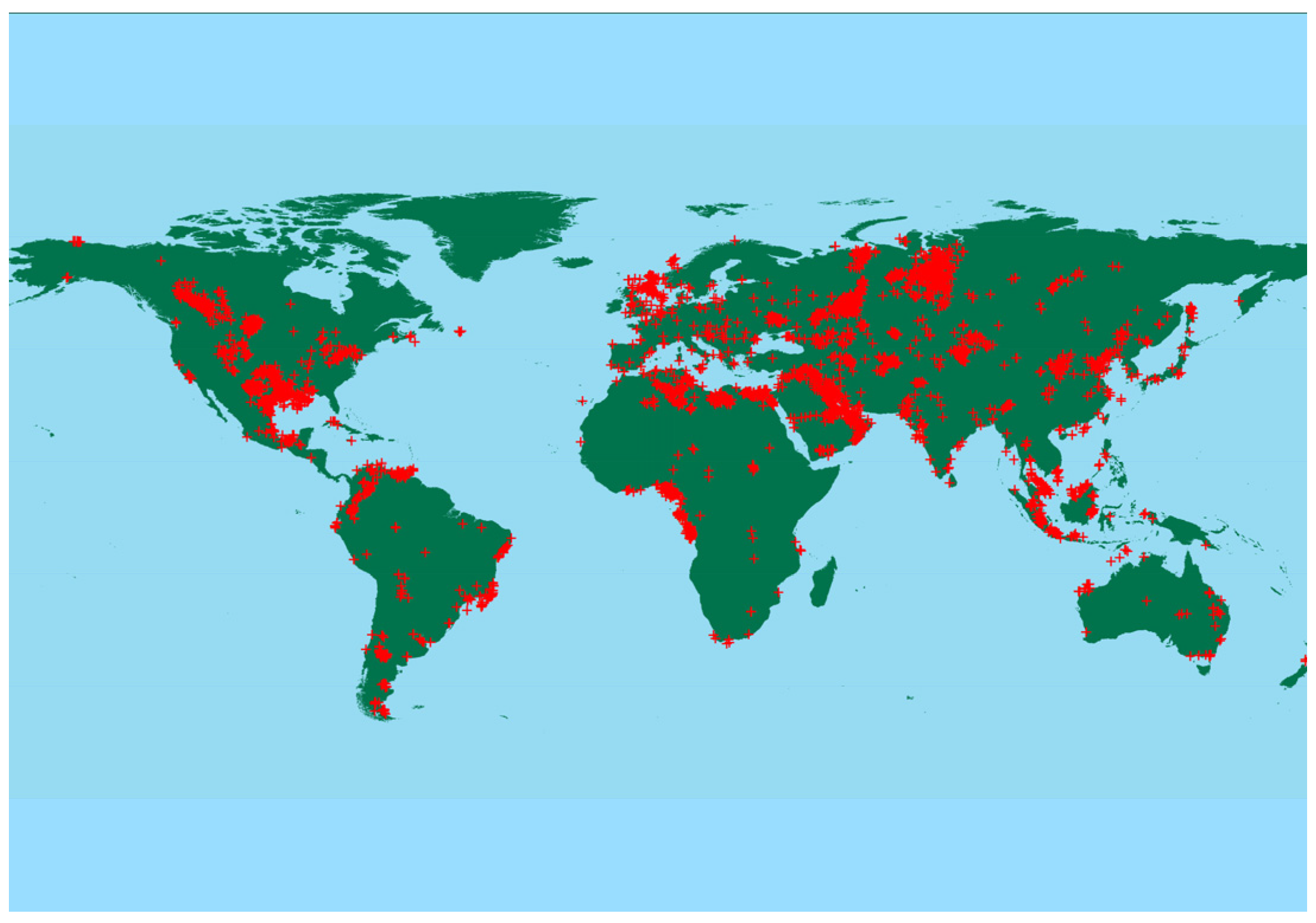
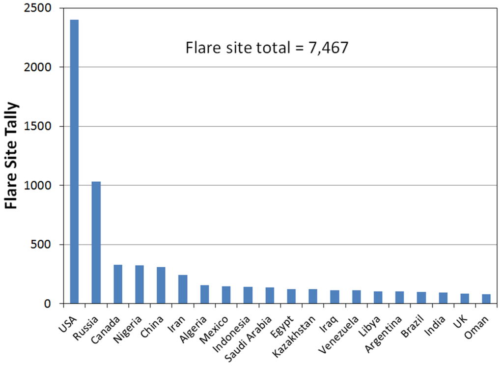
Figure 9. Flare tally by country for 2012.

Figure 9. Flare tally by country for 2012.

4.2. Flared Gas Volume Estimates for Individual Flaring Sites

An output file was generated listing annual flared gas volume estimates for all of the detected flares. The output lists each flare site’s latitude and longitude, average flare temperature, the percent frequency of detection, the normalized sum of RH’ and the annual flared gas volume estimate. In addition to the tabular data, a Keyhole Markup Language (KML) file was produced to enable a review of the results in Google Earth. The KML for 2012 is included as a supplemental file with this publication.

Figure 10 shows the estimated flare volumes for each of the flare sites identified with VIIRS data. It is a classic exponential distribution, with high flare volumes concentrated in a relatively small percentage of the flare sites and large numbers of sites with small flared gas volumes. Half of the flared gas volume is concentrated at fewer than 400 flares, and 90% of the flaring occurs at just 30% of the sites. The largest flare found (Figure 10), located 7 km southeast of Punta de Mata in Venezuela, had an estimated flared gas volume of 1.13 billion cubic meters (BCM). The smallest flare had a 2012 gas flaring volume of 28,431 cubic meters, located in the Lekhwair oil field, Oman. Thus, from smallest to largest, the flared gas volumes mapped by VIIRS span five orders of magnitude.

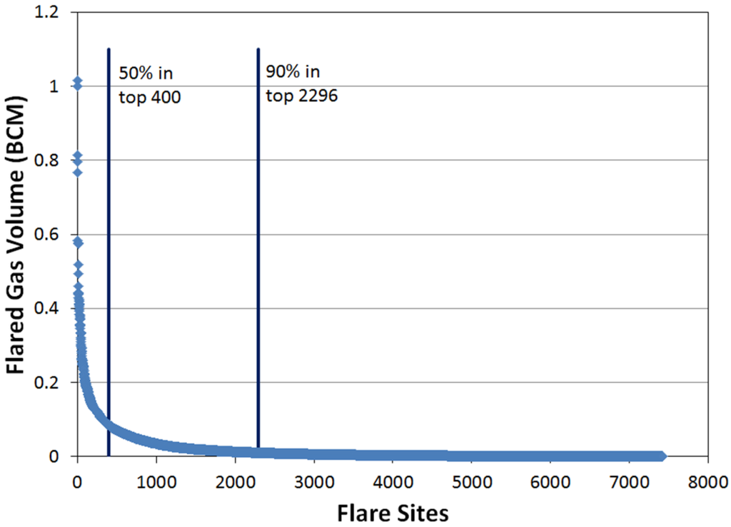
Figure 10. VIIRS estimate flared gas volumes for 7467 gas flares, worldwide. This includes both upstream, downstream and LNG terminal flare sites.

Figure 10. VIIRS estimate flared gas volumes for 7467 gas flares, worldwide. This includes both upstream, downstream and LNG terminal flare sites.

4.3. National- and Global-Level Estimates

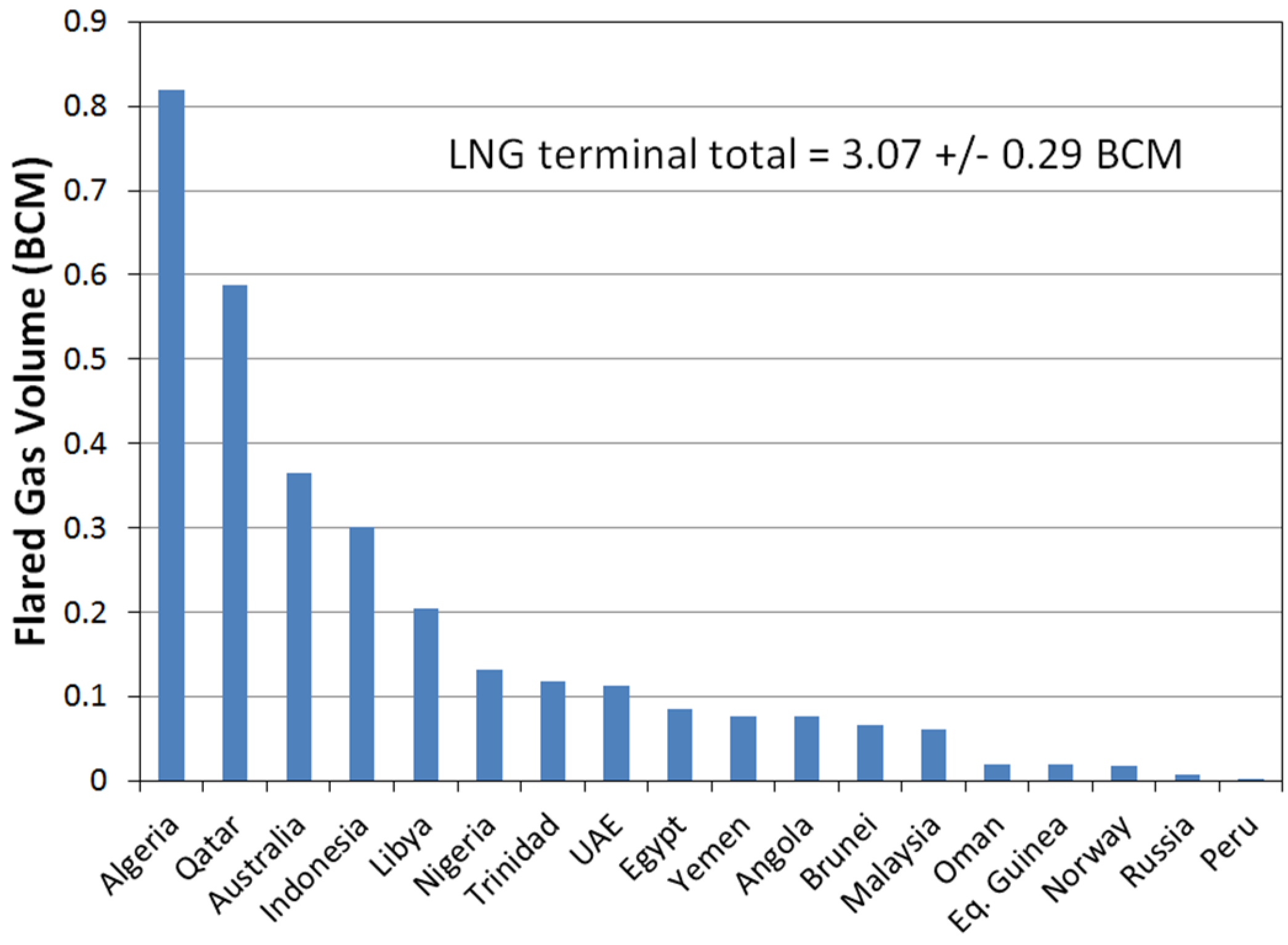
National-level flared gas volumes were calculated by summing the estimates from individual flare sites within the national boundaries and associated exclusive economic zones. The global total flared gas volume is estimated at 143 ± 13.6 BCM. The results can be further divided into upstream, downstream and LNG terminals. Upstream flaring was found in 88 countries; with total flared gas volume in 2012 estimated at 129.4 ± 12.2 BCM (Figure 11). Russia leads in estimated upstream flaring with 24.6 BCM, followed by Iraq (11.9), Iran (10.7), Nigeria (10.5), Venezuela (8.1) and the USA (6.5). Downstream flaring (Figure 12) was found in 85 countries with a total of 10.7 ± 1.0 BCM. Algeria leads in estimated downstream flaring with 1.4 BCM, followed by Iran, Qatar, Mexico and Saudi Arabia. Estimated flaring at LNG liquefaction plants totaled 3.1 ± 0.29 BCM, with Algeria leading with 0.82 BCM (Figure 13).

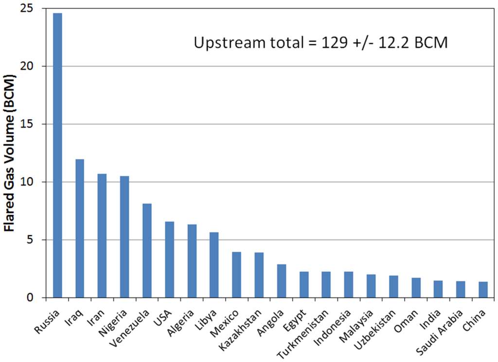
Figure 11. Top 20 countries for upstream gas flaring in 2012.

Figure 11. Top 20 countries for upstream gas flaring in 2012.

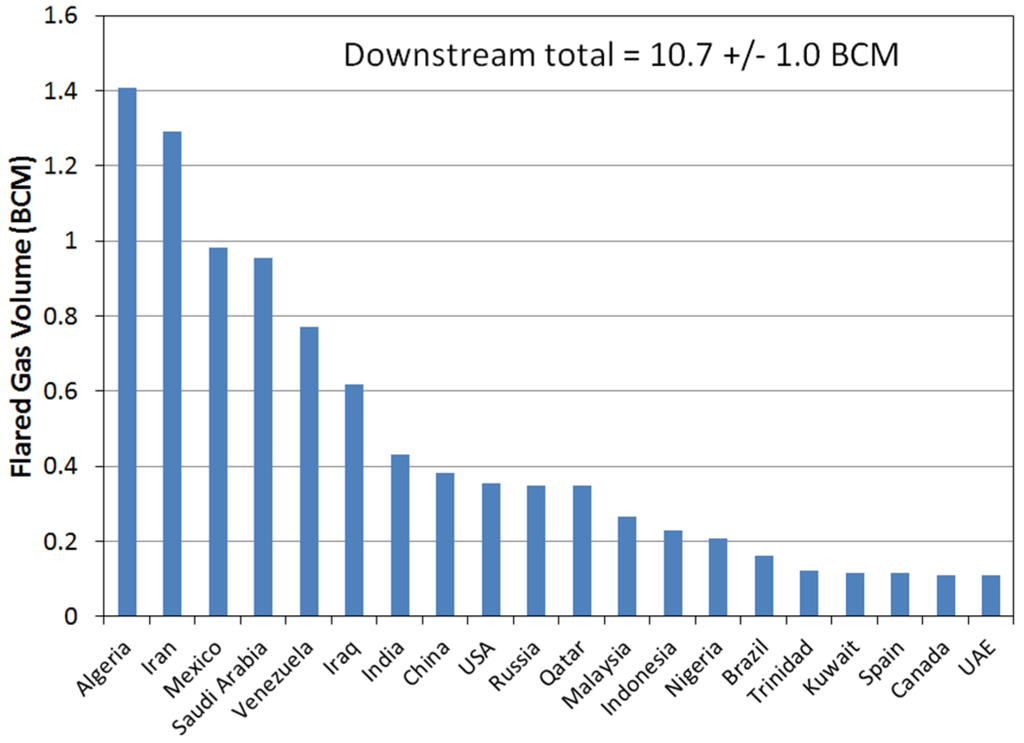
Figure 12. Top 20 countries for downstream gas flaring in 2012.

Figure 12. Top 20 countries for downstream gas flaring in 2012.

Figure 13. 18 countries with LNG terminal gas flaring in 2012.

Figure 13. 18 countries with LNG terminal gas flaring in 2012.

4.4. Comparison with Defense Meteorological Satellite Program Satellite Estimates

The last year where DMSP estimates of flared gas volumes were produced was 2012. DMSP orbit degradation from 2013 onward resulted in solar contamination that made it impossible to produce global data for estimating flared gas volumes.

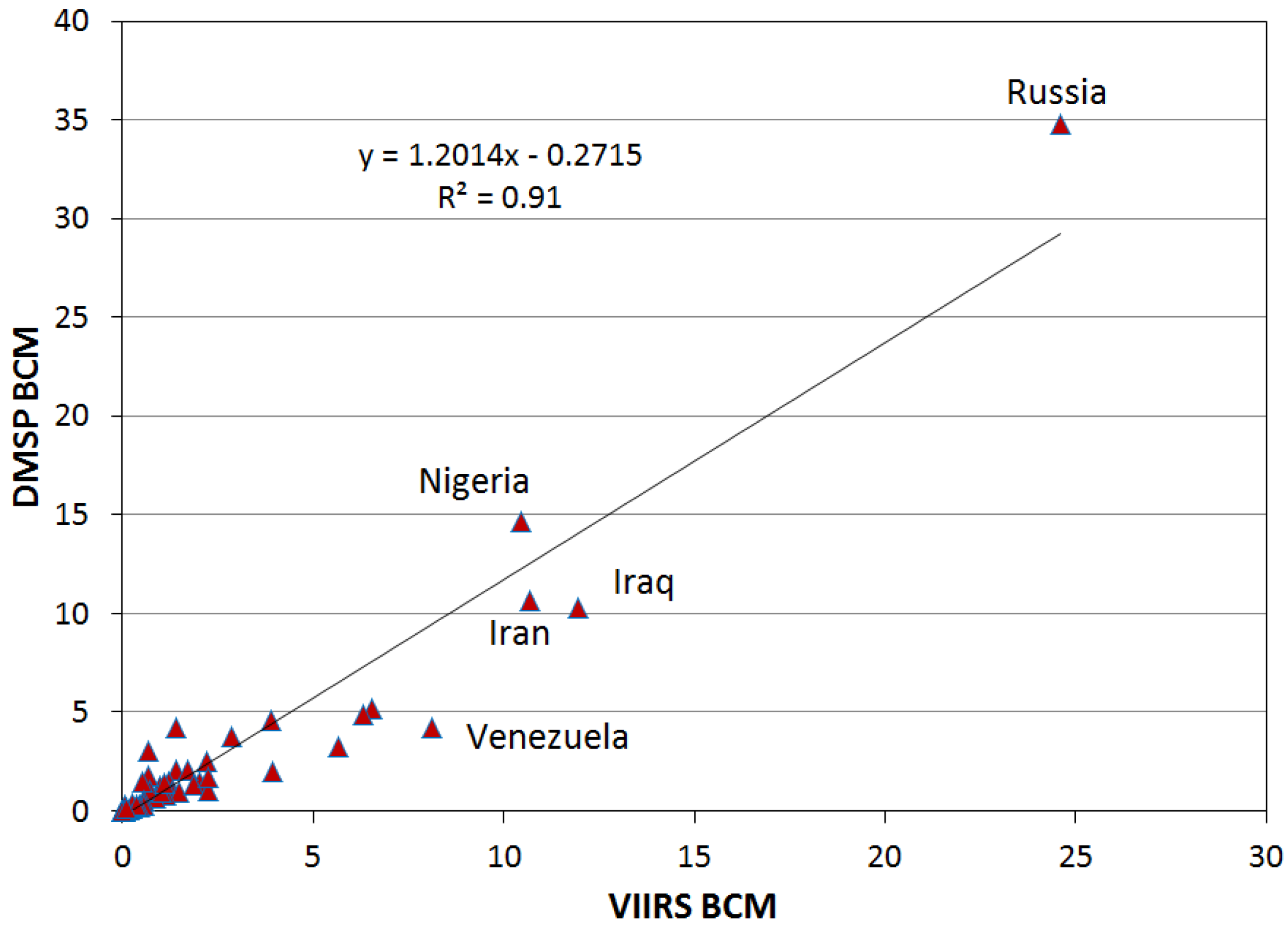
The 2012 global flaring estimate from VIIRS (143 BCM) is 4% higher than the DMSP estimate for the same year (137.4 BCM). The DMSP and VIIRS estimates for individual countries are highly correlated in most cases (Figure 14). There are several factors that may be contributing to the differences between the flared gas volume estimates between DMSP and VIIRS. Firstly, the DMSP sensor sensitivity to electric lighting made it impossible to identify gas flares imbedded in urban areas. VIIRS does not suffer from this drawback and has identified a substantial number of flaring sites that could not be identified in DMSP data. Secondly, the DMSP’s inability to distinguish between flare radiant emissions and electric lighting may have resulted in overestimates of flared gas volumes at heavily lit locations. Third, the center core of many gas flaring detections made with DMSP were saturated, meaning that the signal was truncated by the limited dynamic range of the DMSP instrument. In contrast, no saturation was encountered in gas flare observations in the M10 spectral band. Fourth, the DMSP low light imaging data have no in-flight calibration. An empirical intercalibration was used to reduce sensor differences in the flared gas estimation [7]. This issue is resolved with VIIRS, which is widely regarded as a well calibrated instrument. Fifth, the DMSP calibration for estimating flared gas volumes excluded Russian data, since it was impossible to separate flaring in oil versus gas areas at that time due to the lack of field-specific vectors. Finally, the multispectral VIIRS data provides samples across 99% of the Planck curve modelling of a flare’s radiant energy, as compared to 2% with the single DMSP band.

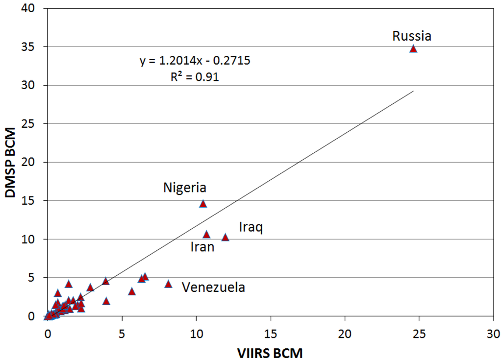
Figure 14. VIIRS versus DMSP flared gas estimates for 2012.

Figure 14. VIIRS versus DMSP flared gas estimates for 2012.

5. Conclusions

Using a series of processing steps, it is now possible to conduct global surveys to identify gas flaring sites and estimate flared gas volumes using nighttime VIIRS data. A survey of global gas flaring in 2012 found 7467 flaring sites worldwide, with an estimated 143 (±13.6) BCM of flared gas volume. The quantity of upstream (production related) flaring was estimated at 129.4 (±12.2) BCM, downstream flaring at 10.7 (±1.01) BCM and flaring at LNG liquefaction plants estimated at 3.07 (±0.29) BCM. While the USA had the largest number of individual flare sites, Russia led in terms of the largest flaring volume.

The VIIRS instrument has substantial advantages over other satellite sensors in terms of global monitoring of gas flaring. VIIRS collects global data every 24 h, providing repeat observations that enable numerous cloud-free observations of each site to be made over the course of a year. VIIRS is unique in the collection of near-infrared and SWIR data at night that has proven to be extremely useful for detecting flares and measuring their radiant output. The VIIRS M10 spectral band, centered at 1.6 µm, covers the peak radiant emissions for gas flares. The other two bands that collect at night are at 0.75 and 0.9 µm, recording radiances on the leading edge of gas flaring radiant emissions. At night, these three spectral bands record unambiguous radiant emissions from gas flares and other hot sources. These are augmented with radiance measurements from two traditional fire detection spectral bands in the 4-µm region. Planck curve fitting of the hot source radiances yields estimates of the temperature (K), source size (m²) and, hence, RH (MW) of the hot sources. Flares can be distinguished from other hot sources based on their high temperature and persistence.

While VIIRS has a substantial number of favorable characteristics, it has two primary shortcomings of which the data users should be aware. The first shortcoming is the inability to derive temperature, source size and RH for weak detections made on small gas flares. The Planck curve fitting requires detection radiances in at least two spectral bands. There is a class of small flares where detection occurs only in the M10 spectral band, the location of the peak radiant emissions from most flares. These M10-only events can also arise from biomass burning and industrial sites. With no Planck curve fit, there is no direct calculation for RH. We developed methods to assign temperatures to the M10-only detections; however, these observations are not as good as the multispectral Planck curve fit observations. This single band detection problem on small gas flares will be resolved when nighttime M11 collections are added to the VIIRS data stream.

The second shortcoming arises from the temporal sampling limitations of the VIIRS instrument. VIIRS collects global data every night, but the dwell time of VIIRS on a flaring site is a fraction of a second. For steady and continuous flares, this temporal sampling appears to be adequate. However, VIIRS under-samples intermittent or rarely active flares. This under-sampling lowers the probability of detection and decreases the accuracy of flared gas estimates for flares with highly variable flared gas volumes.

We investigated the impact of applying an atmospheric correction using two flares in a humid tropical environment (onshore and offshore) and one flare in a dry desert environment. The atmospheric correction boosted the RH, but the effects across the three sites were highly linear. Our conclusion is that no atmospheric correction is required for gas flare detection made with the Nightfire algorithm. We attribute this to the high transmissivity of the atmosphere in the 1.6 μm window, where the gas flares typically have their highest radiant output.

Gas flares tend to be taller than they are wide due to the buoyancy of the heated air mass. Because VIIRS views gas flaring sites over a wide range of view angles, a substantial portion of the variation in RH estimates can be attributed to the viewed source size varying as a function of view angle. We developed a method for characterizing the average ellipticity of individual flares by analyzing the source size as a function of satellite zenith angle. We use the ellipticity to estimate the source size for all flares as viewed from the horizontal, which presents the largest apparent source area. This increases the coefficient of determination (R²) in the calibration to estimate flared gas volumes.

A calibration for estimating flared gas volumes has been developed based on national-level data for upstream flaring reported by Cedigaz. For this calibration, the VIIRS data for Russia were filtered to only include flares at oil production facilities, since this is the only type of flaring reported in the Cedigaz data.

Despite the good correlation for many countries, there remains a considerable spread between the Cedigaz reported data and the VIIRS observed RH (Figure 7). For instance, the Cedigaz estimate for Iran (17.55 BCM) is high relative to the observed RH'. As a result, the VIIRS estimated flared gas volume for Iran (12.54 BCM) is 29% lower than the Cedigaz number. Other countries where the VIIRS estimates are lower than the Cedigaz numbers include Nigeria, Venezuela, the USA, Angola and Indonesia. Countries where the VIIRS estimates are higher than the Cedigaz numbers include Russia, Iraq, Libya and Algeria. In the future, it may be possible to improve the VIIRS gas flaring calibration using observations of flaring sites with metered flare volumes spanning a substantial portion of the range found in the VIIRS data.

This paper reports on results for the year 2012. Results from 2013, 2014 and 2015 will be available in the near future. The VIIRS data on flared gas volumes should be useful in carbon cycle studies, identification of sites for natural gas utilization projects, calculating carbon intensities of fuels and tracking the progress of efforts to reduce gas flaring. Such projects can rely on the availability of VIIRS data from NOAA for the next several decades.

Because flaring burns off a potentially valuable fuel commodity, it is one of the obvious places to focus efforts to reduce the carbon loading on the atmosphere as it represents. Making use of natural gas that would otherwise be flared could reduce the consumption of other fuels, thus lowering the total volume of carbon emissions to the atmosphere. Flared gas volume represents about 3.5% of total worldwide natural gas consumption and 19.8% of U.S. natural gas consumption in 2012 [15]. If used to fuel vehicles, it could power 74 million automobiles in the USA based on an average of 25 miles per gallon of gasoline [16] and 13,476 miles per year [17].

In summary, we have developed a systematic set of algorithms and methods that can be used on a repeated basis to identify gas flaring sites worldwide, with estimation of flared gas volumes. With this capability, VIIRS can provide detailed, site-specific data for tracking efforts to reduce natural gas flaring.

References

- Peylin, P.; Law, R.M.; Gurney, K.R.; Chevallier, F.; Jacobson, A.R.; Maki, T.; Niwa, Y.; Patra, P.K.; Peters, W.; Rayner, P.J.; et al. Global Atmospheric Carbon Budget: Results from an ensemble of atmospheric CO2 inversions. Biogeosciences 2013, 10, 6699–6720. [Google Scholar] [CrossRef]
- Sonibare, J.A.; Akeredolu, F.A. Natural gas domestic market development for total elimination of routine flares in Nigeria’s upstream petroleum operations. Energy Policy 2006, 34, 743–753. [Google Scholar] [CrossRef]
- Sonia, Y.; Witcover, J.; Kessler, J. Status Review of California’s Low Carbon Fuel Standard—Spring 2013 Issue; Research Report UCD-ITS-RR-13-06; Institute of Transportation Studies, University of California: Davis, CA, USA, 2013. [Google Scholar]
- Anejionu, O.C.D.; Blackburn, G.A.; Whyatt, J.D. Detecting gas flares and estimating flaring volumes at individual flow stations using MODIS data. Remote Sens. Environ. 2014, 158, 81–94. [Google Scholar] [CrossRef]
- Casadio, S.; Arino, O.; Serpe, D. Gas flaring monitoring from space using the ATSR instrument series. Remote Sens. Environ. 2012, 116, 239–249. [Google Scholar] [CrossRef]
- Chowdhury, S.; Shipman, T.; Chao, D.; Elvidge, C.D.; Zhizhin, M.; Hsu, F.-C. Daytime gas flare detection using Landsat-8 multispectral data. In Proceedings of the IEEE International Geoscience Remote Sensing Symposium, Quebec City, QC, Canada, 13–18 July 2014; pp. 258–261.
- Elvidge, C.D.; Ziskin, D.; Baugh, K.E.; Tuttle, B.T.; Ghosh, T.; Pack, D.W.; Erwin, E.H.; Zhizhin, M. A Fifteen Year Record of Global Natural Gas Flaring Derived from Satellite Data. Energies 2009, 2, 595–622. [Google Scholar] [CrossRef]
- Elvidge, C.D.; Zhizhin, M.; Hsu, F.-C.; Baugh, K.E. VIIRS Nightfire: Satellite Pyrometry at Night. Remote Sens. 2013, 5, 4423–4449. [Google Scholar] [CrossRef]
- Giglio, L.; Descloitres, J.; Justice, C.O.; Kaufman, Y.J. An enhanced contextual fire detection algorithm for MODIS. Remote Sens. Environ. 2003, 87, 273–282. [Google Scholar] [CrossRef]
- Kopp, T.J.; Thomas, W.; Heidinger, A.K.; Botambekov, D.; Frey, R.A.; Hutchison, K.D.; Iisager, B.D.; Brueske, K.; Reed, B. The VIIRS Cloud Mask: Progress in the first year of S-NPP toward a common cloud detection scheme. J. Geophys. Res. Atmos. 2014, 119, 2441–2456. [Google Scholar] [CrossRef]
- Berk, A.; Anderson, G.P.; Acharya, P.K.; Shettle, E.P. MODTRAN 5.2. 1 User’s Manual; Spectral Sciences Inc.: Burlington, MA, USA; Air Force Research Laboratory: Hanscom Air Force Base, MA, USA, 2011. [Google Scholar]
- Jekrard, H.G. Transmission of Light through Birefringent and Optically Active Media: The Poincaré Sphere. J. Opt. Soc. Am. 1954, 44, 634–640. [Google Scholar] [CrossRef]
- ArcGIS Shapefiles for Global Crude Oil Refinereis and LNG Liquifaction Terminals; Environmental Systems Research Institute (ESRI): Redlands, CA, USA, 2014.
- Cedigaz National Flared Gas Volumes. Available online: http://www.cedigaz.org/products/natural-gas-database.aspx (accessed on 8 September 2015).
- Natural Gas Statistics, U.S. Energy Information Administration. Available online: http://www.eia.gov (accessed on 25 October 2015).
- Monthly Monitoring of Vehicle Fuel Economy and Emissions. University of Michigan, Transportation Research Institute. Available online: http://www.umich.edu/~umtriswt/EDI_sales-weighted-mpg.html (accessed on 7 December 2015).
- Average Annual Miles per Driver by Age Group. Department of Tranportation, Federal Highway Administration. Available online: https://www.fhwa.dot.gov/ohim/onh00/bar8.htm (accessed on 7 December 2015).
© 2015 by the authors; licensee MDPI, Basel, Switzerland. This article is an open access article distributed under the terms and conditions of the Creative Commons by Attribution (CC-BY) license (http://creativecommons.org/licenses/by/4.0/).