5.1. Scenario 1: Simulation under Constant Ambient Temperature Conditions
A population of ACs of similar characteristics can be used as a control group [
22,
23]. We choose the downtown area of the city of Nanjing, China for this research, where there are 18,000 ACs of 10,000 residents participating in the demand response plan. Parameters of ACs in the group are as follows: thermal resistance
, thermal capacitance
, thermal power
. When the ambient temperature is constant (e.g., 32 °C), the parameters of the two order transfer function of the aggregate AC group are shown in
Table 2. In this scenario the parameters remain unchanged.
First, we do not have any control over the AC population. Therefore the temperature set point would stay fairly stable, and the total power demand of the whole AC population is shown in
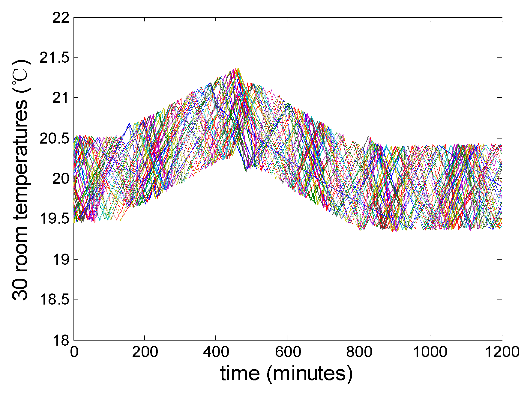
Figure 10. The temperature of 30 random air-conditioned rooms among the population is presented in
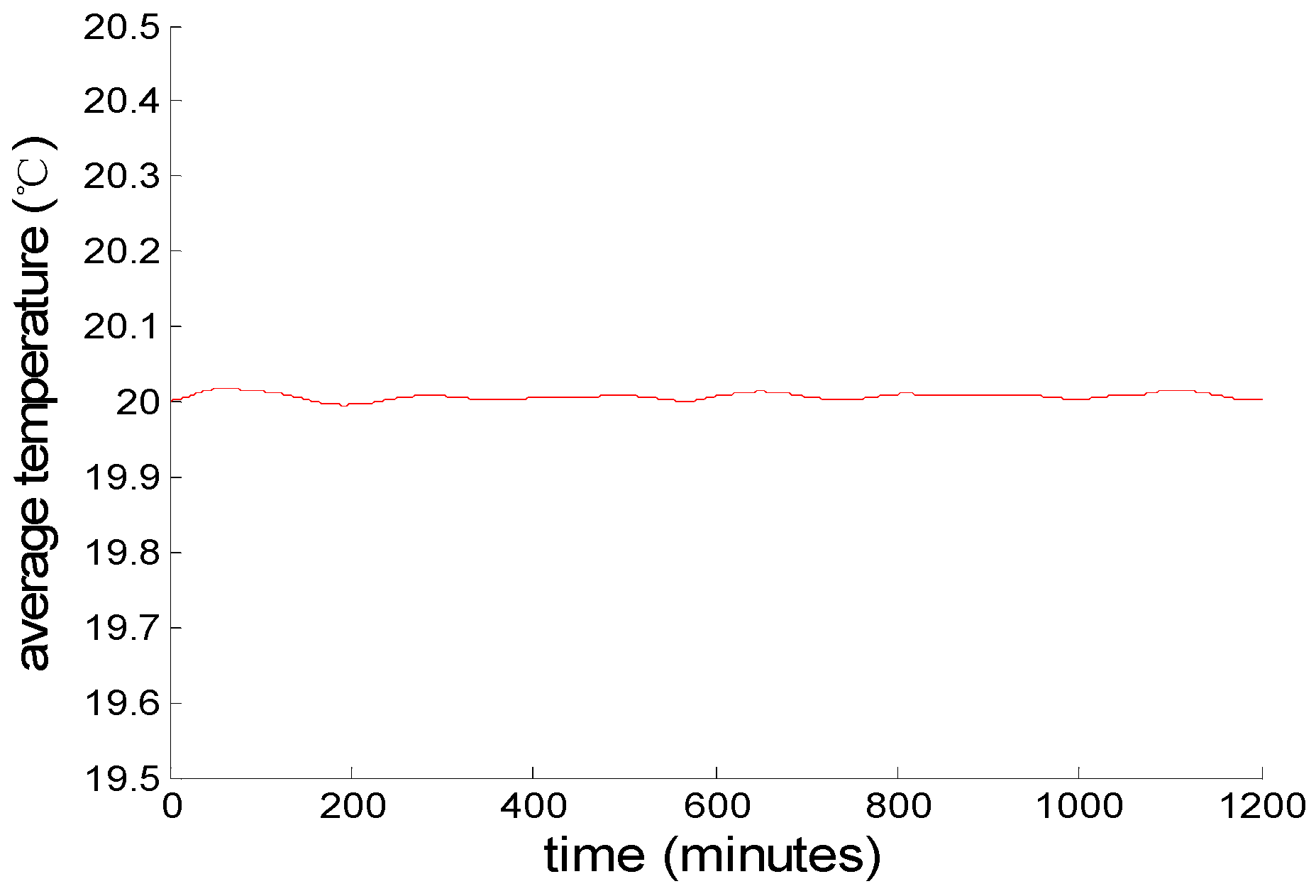
Figure 11, and the mean temperature inside the house of all ACs is presented in
Figure 12. The simulations were run in MATLAB (The MathWorks, Inc., Natick, MA, USA.) on a desktop computer equipped with an Intel Corei5-3230M 2.60GHz CPU, 4.00 GB memory, and 64 bit Windows 8 operating system.
Figure 10,
Figure 11 and
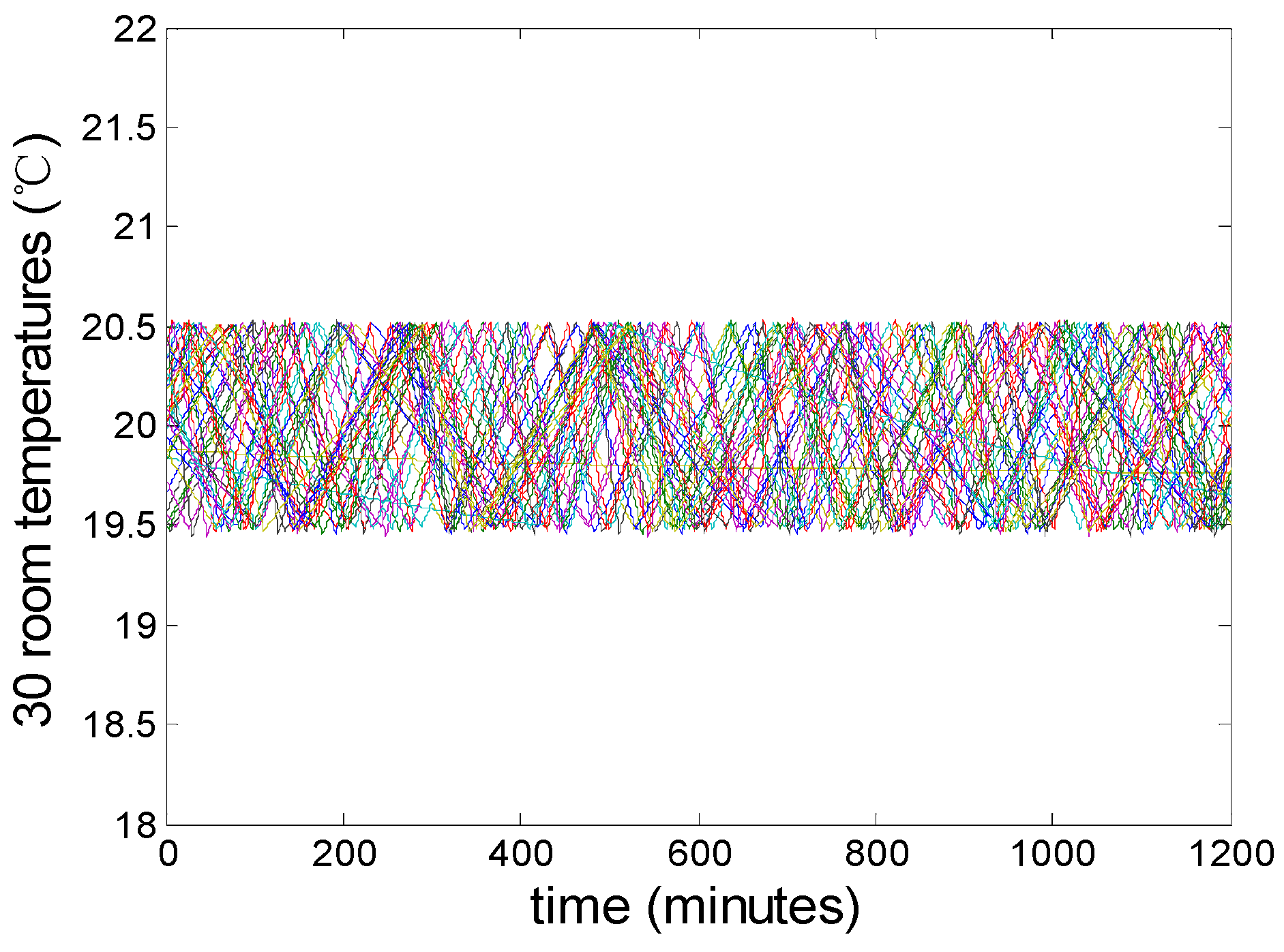
Figure 12 show that, without any control, the AC group will keep running independently. The profile of the aggregated demand of AC group is gentle, the duty cycle in steady state is 0.467. The temperatures of 18,000 air-conditioned rooms are uniformly distributed between 19.5–20.5 °C. The hysteresis width, which determines the upper and lower limits of temperature inside the air-conditioned rooms, is 1 °C. Besides, the mean temperature of all AC rooms is close to the temperature set point 20 °C.
A scenario analysis by varying the temperature set point offset to control the aggregated power demand of air-conditionings is started. Assuming that at the initial stage, 44.6% of the ACs are on, while the rest of them are off, the whole load control scenario is divided into three stages. For the first 100 min, the ACs run independently without any control. The second stage is from 100 to 350 min, during which the grid is in a peak load period. There is a power shortage and therefore needs a 20% reduction of air conditioning load, which is equivalent to 4.3 MW. The load aggregator will raise the temperature set point of the ACs to achieve peak load shifting. The third stage takes place between 350 and 600 min, when the peak load period of the power grid is over, it needs an additional 20% increase of air conditioning load to meet the power consumption of the off-peak period. The load aggregator will drop the temperature set point of the ACs to achieve a satisfactory comfort level. The load management scenario finalizes at
t = 600 min. In this scenario, the two order transfer function of the AC group remains unchanged because of the constant ambient temperature, as is shown in
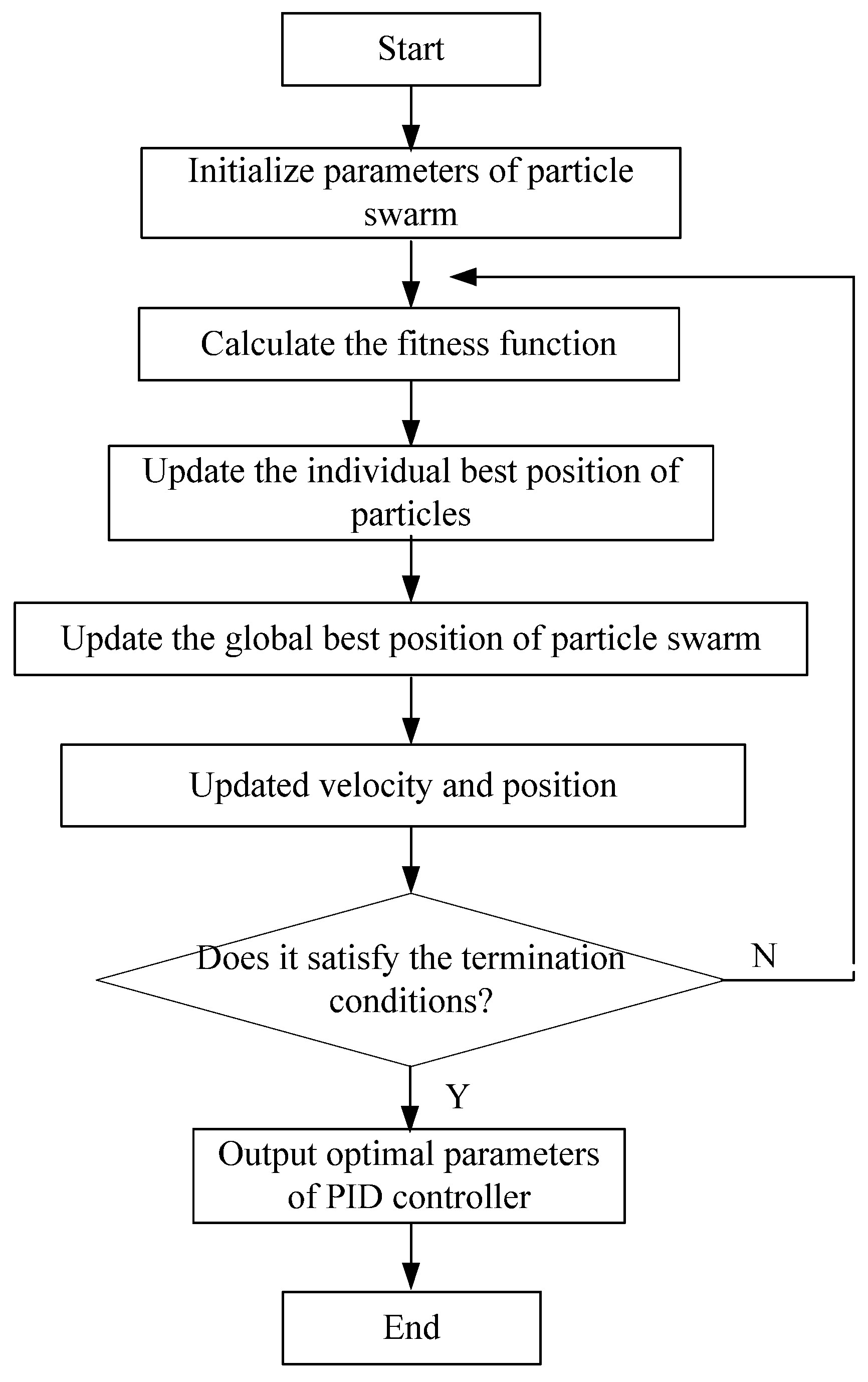
Table 2. The particle swarm optimization algorithm is applied to tune parameters for the PID controller. The parameters of the PSO algorithm are set as follows: population size
m = 100, dimension
D = 3, the 3 parameters
Kp,
Ki and
Kd, to be optimized are in the range of 0–300, the inertia weight
w = 0.6, the maximum number of iterations
t = 200, acceleration coefficients
.
Figure 10.
Total power demand of the whole AC population.
Figure 10.
Total power demand of the whole AC population.
Figure 11.
The temperature of 30 random air-conditioned rooms among the population.
Figure 11.
The temperature of 30 random air-conditioned rooms among the population.
Figure 12.
The mean temperature inside the houses of all ACs.
Figure 12.
The mean temperature inside the houses of all ACs.
The IEAT index is chosen as the fitness function, with the minimum fitness value being 0.1. The particle velocity is between [−1, 1]. How to select the parameters of the PSO algorithm in detail is explained in [
24,
25].
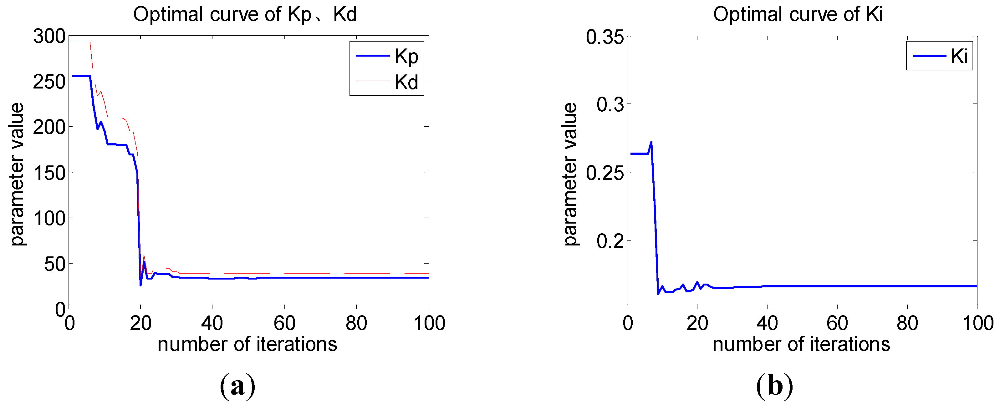
Figure 13a,b shows the optimization of PID parameters
Kp,
Ki and
Kd by using the PSO algorithm, and
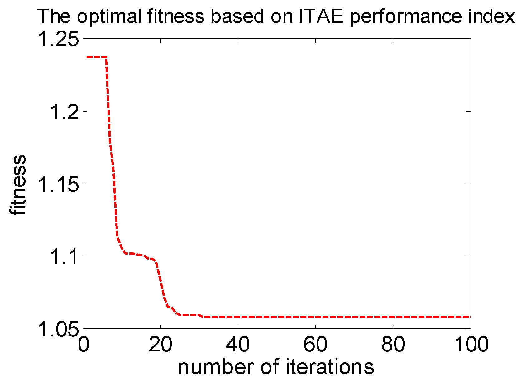
Figure 14 shows a variation of the ITAE performance index.
Figure 13.
The optimization of PID parameters by using PSO algorithm. (a) Kp, Kd; (b) Ki.
Figure 13.
The optimization of PID parameters by using PSO algorithm. (a) Kp, Kd; (b) Ki.
Figure 14.
A variation of the integrated time and absolute error (ITAE) performance index.
Figure 14.
A variation of the integrated time and absolute error (ITAE) performance index.
With the increase of the number of iterations of the particle swarm, the ITAE performance index, which is considered as the fitness function, gradually stabilizes at around 1.06. Therefore, we get the optimal PID parameters and the performance index as shown in
Table 3, in which we tune PID parameters by using the particle swarm optimization algorithm and make a comparison of tuning results with the Ziegler-Nichols method. The parameters
ts represents settling time, and
tp represents peak time. In order to demonstrate the advantages of the PSO algorithm, we compared it with the classical Ziegler-Nichols method on tuning PID parameters of the two order transfer function model for aggregated ACs [
26]. Simulation results indicate that, although the peak time of the tuning process is slightly longer, the optimized controller based on the PSO algorithm outperforms the conventional one greatly in the settling time, overshoot and performance index.
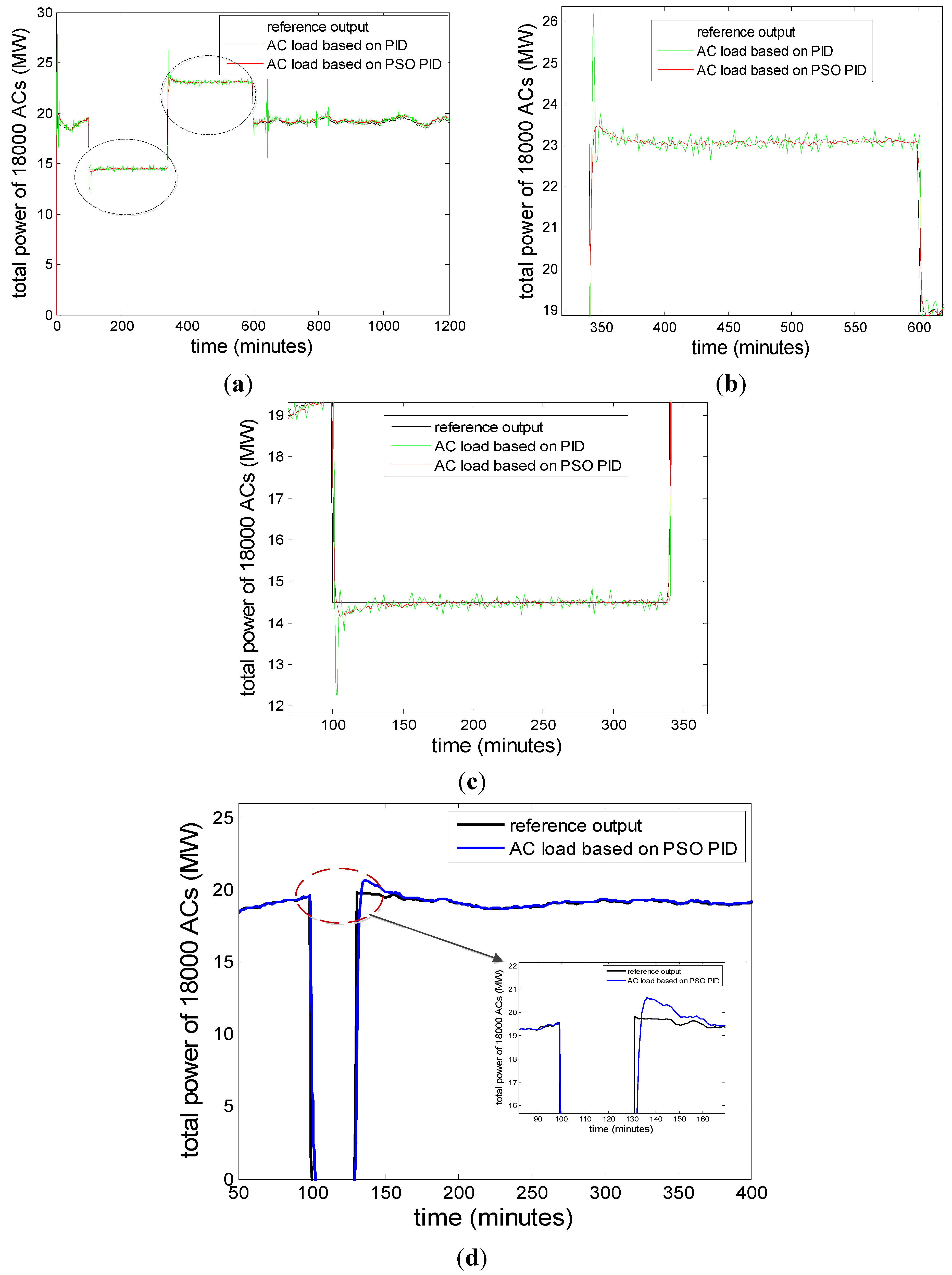
Figure 15 shows the comparison between the desired reference value of the aggregated demand of a population of ACs for load shifting, the power output of the population based on conventional PID controller, and the power output of the population based on PSO tuning PID parameters, when the outdoor temperature is a constant 32 °C. In
Figure 15, the black curve is the ideal load control reference output, the green curve is the actual power output of the population using the Ziegler-Nichols method to tune PID parameters, and the red curve is the actual power output of the population using the particle swarm optimization algorithm to tune PID parameters.
Figure 15b,c is obtained by zooming in on the parts circled by a dotted curve in
Figure 15a, and show the effects of reducing the power output in 100–350 min and increasing the power output in 350–600 min, respectively.
Table 3.
Tuning proportional-integral-differential (PID) parameters using the Ziegler-Nichols method in comparison with the particle swarm optimization algorithm.
Table 3.
Tuning proportional-integral-differential (PID) parameters using the Ziegler-Nichols method in comparison with the particle swarm optimization algorithm.
| Parameters | PID Tuning Methods |
|---|
| Classic Z-N Algorithm | Particle Swarm Optimization (PSO) |
|---|
| 26.521 | 33.647 |
| 0.023 | 0.167 |
| 10.870 | 38.799 |
| 30.596% | 3.115% |
| 26.704 | 18.363 |
| 5.800 | 7.318 |
| Integrated Time and Absolute Error (ITAE) | 4.292 | 1.060 |
As can be seen from the figure, using PSO to tune PID parameters is significantly better than using the Z-N algorithm. In response to the step changes of reference values of load control at time 100 and 350 min, the Z-N tuning method has a larger overshoot, a longer settling time, a continuous oscillation throughout the control process and more glitches. In contrast, the control effect on PSO algorithm tuning PID parameters is quite satisfactory, and it meets with requires of rapidity, accuracy and stability of the control system.
We can also achieve a 100% load reduction by adjusting the expected reference value of the air conditioning load to zero.
Figure 15d shows the simulation results of the aggregated demand of n ACs in this extreme case. We assume that, there appears a serious power shortage and needs a 100% reduction of air conditioning load. The aggregated power consumption of ACs based on PSO tuning PID parameters drops to zero when the reference signal is applied at time
t = 100 min, and the whole stage continues for 30 min.
The cost of doing so is that all of the ACs have been switched off and the air temperature inside the house will gradually rise. From a technological perspective, we can achieve any arbitrary adjustment of ACs by using the proposed model and control strategy, but in a real-world scenario, if the duration of 100% load reduction is longer, it will affect the user’s comfort and lead to their dissatisfaction on a hot day. Thirty min later, the power demand increases to the initial value, and all of ACs return to the steady state without any parasitic oscillation.
Figure 16 shows the variation of the indoor temperature of 30 random ACs. The temperature hysteresis width
H = 1 °C. The air temperature inside the house changes in response to the variation of the temperature set point
u(
t). We also observe that, the ACs’ temperature set point can be controlled by the load aggregator who sets a higher value to reduce the load, as well as setting a lower value to increase the load. After 600 min, the control process is over, but the room temperature does not directly return to the initial value [19.5 °C, 20.5 °C]. Instead, it has undergone a nearly 200 min variable process, and the final stable temperature is slightly lower than the initial value. The reason for this phenomenon is that the characteristics of air conditioning itself make the load rebound before and after the load control event.
Figure 15.
(a), (b), (c) A comparison between the desired reference value of the aggregated demand of a population of ACs for load shifting, the power output of the population based on conventional PID controller, and the power output of the population based on PSO tuning PID parameters, when the outdoor temperature is constantly 32 °C. (d) The aggregated demand of n ACs in the extreme case of a 100% load reduction for 30 min.
Figure 16.
Variation of the indoor temperature of 30 random ACs in the population.
Figure 16.
Variation of the indoor temperature of 30 random ACs in the population.
Mehta
et al., proposed an advanced open loop method in [
27,
28,
29], which reduced two-way broadcasting to one-way and eliminated the problem of unwanted synchronization of TCLs with high quality control and without requiring a channel for consumer-to-grid communication. To quickly compensate for a mismatch between generation and load, the authors put forward strategies based on the timer-based safe protocols (SPs), including SP-1, SP-2 and SP-3, and focus on developing the algorithms to generate a set of power pulses that are useful in spinning reserve applications.
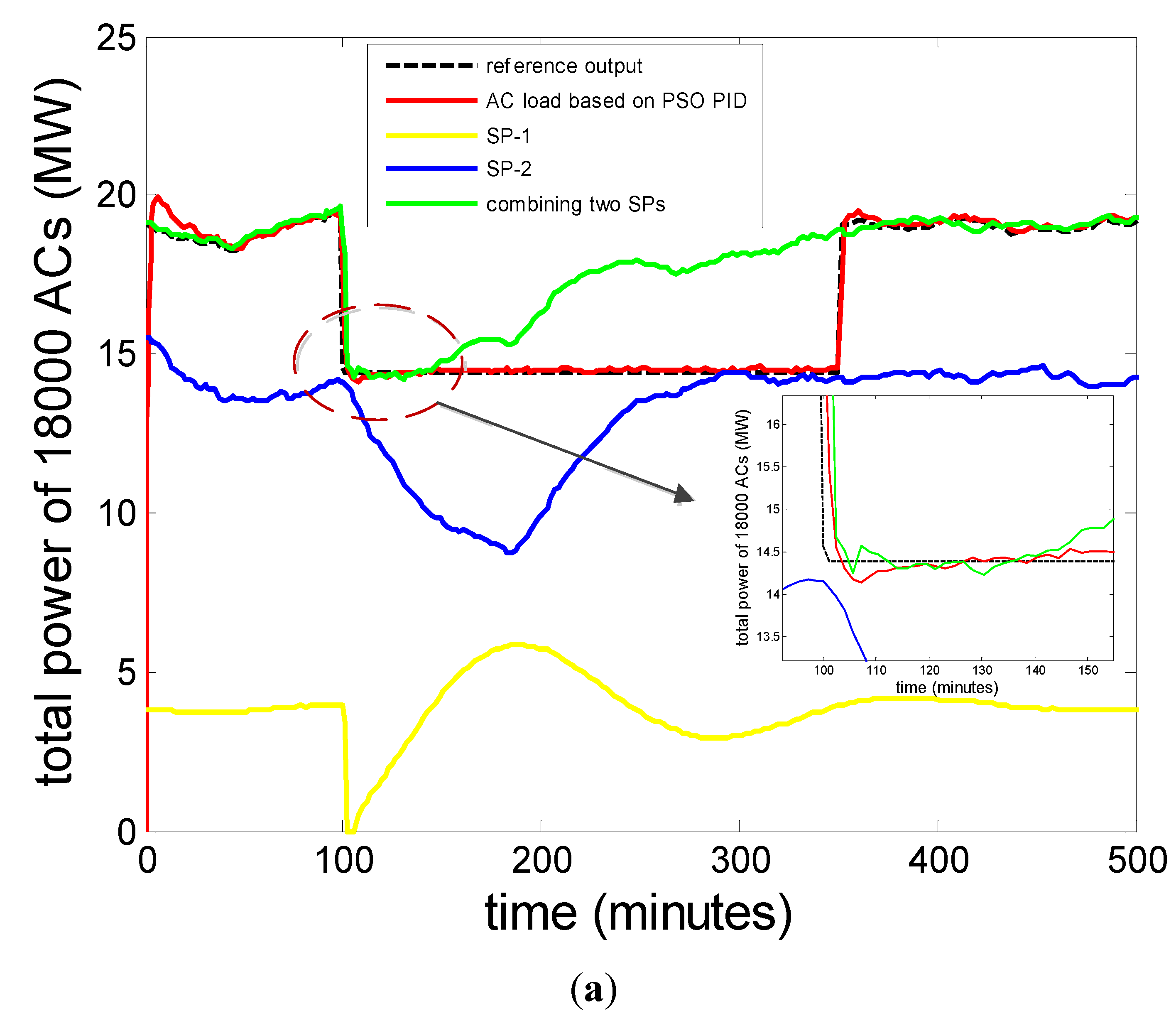
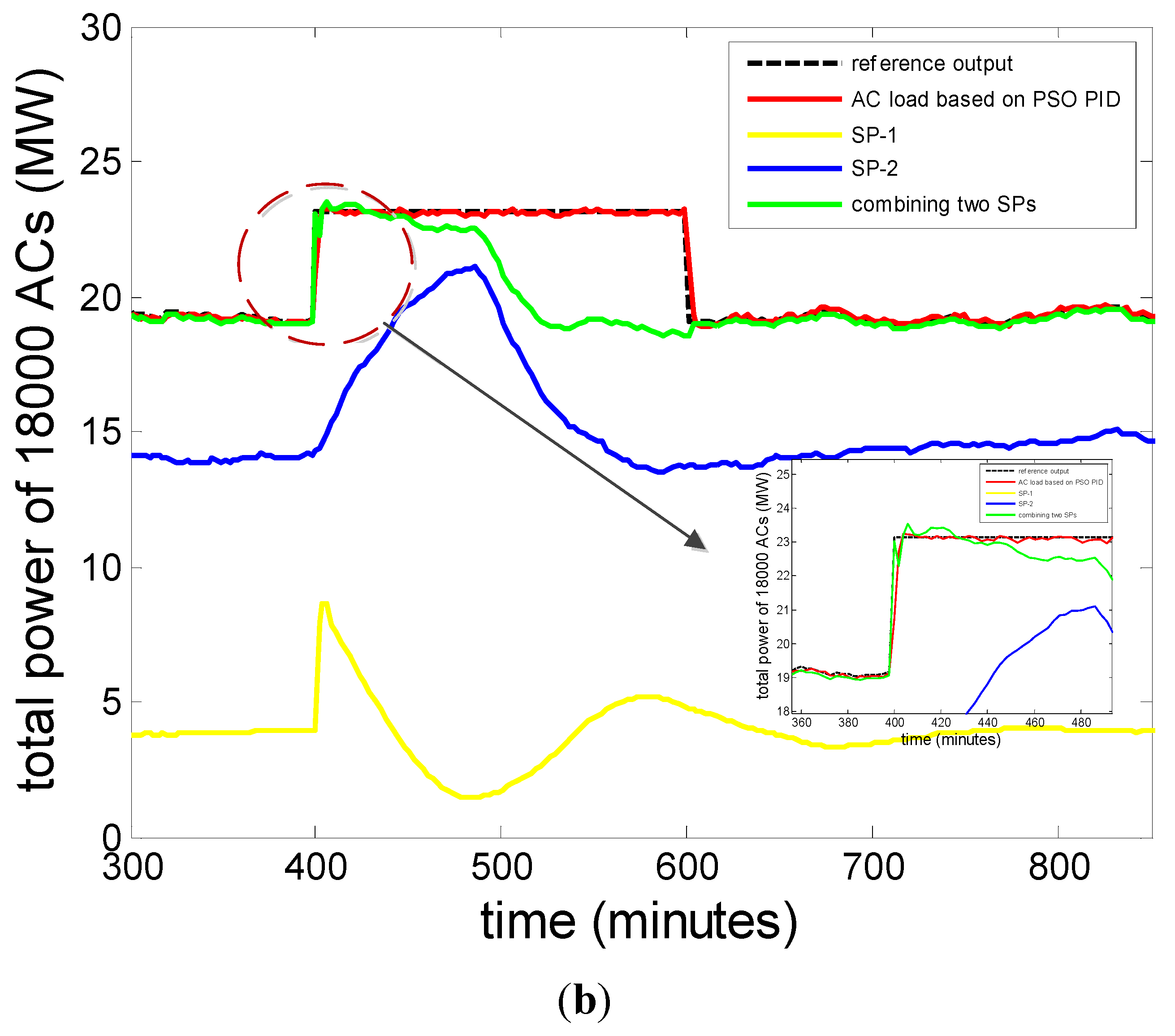
This paper presents a comparison of power demand response between the above hybrid SP protocol combining SP-1 and SP-2 and the proposed closed loop strategy in
Figure 17. The simulation scenario is unchanged, from 100 to 350 min, there needs a 20% reduction of air conditioning load (
Figure 17a), and an additional 20% increase of air conditioning load to meet the power consumption of the off-peak period (
Figure 17b).
Figure 17.
A comparison of power demand response between the proposed closed loop strategy and hybrid SP protocol combining SP-1 and SP-2. (a) Negative pulse: p = 0.2, ξ = 0.5 °C; (b) Positive pulse: p = 0.2, ξ = −0.5 °C.
Figure 17.
A comparison of power demand response between the proposed closed loop strategy and hybrid SP protocol combining SP-1 and SP-2. (a) Negative pulse: p = 0.2, ξ = 0.5 °C; (b) Positive pulse: p = 0.2, ξ = −0.5 °C.
The green line is the power response under hybrid SP protocol which combines SP-1 (yellow) and SP-2 (blue). How these protocols work in detail is explained in [
28,
29]. The proportion of the ACs undergoing SP-1 is
P = 0.2, and the rest of them follows SP-2. By combining two SPs, peak reduction can be achieved. It can be observed that from 100 to 160 min, and from 400 to 600 min, the power demand of ACs based on the hybrid protocol combing two SPs has been tracking the reference output closely. It responded to the signal instantly and maintained the low power at the expected value for an hour (the natural TCL cycle time), but in the remaining time, the green curve gradually deviates from the reference value, and is slowly saturating close to the initial value. In contrast, at all times during the control period (100–350 min and 400–600 min), the power demand curve based on the proposed model and control strategy (red) is tightly maintained.
Although there are many advantages, the SP strategy is an open loop approach, and cannot compensate for the output error. On the contrary, the proposed closed loop control can adjust the control signal according to the results to obtain a higher precision.
5.2. Scenario 2: Simulation under Variable Ambient Temperature Conditions
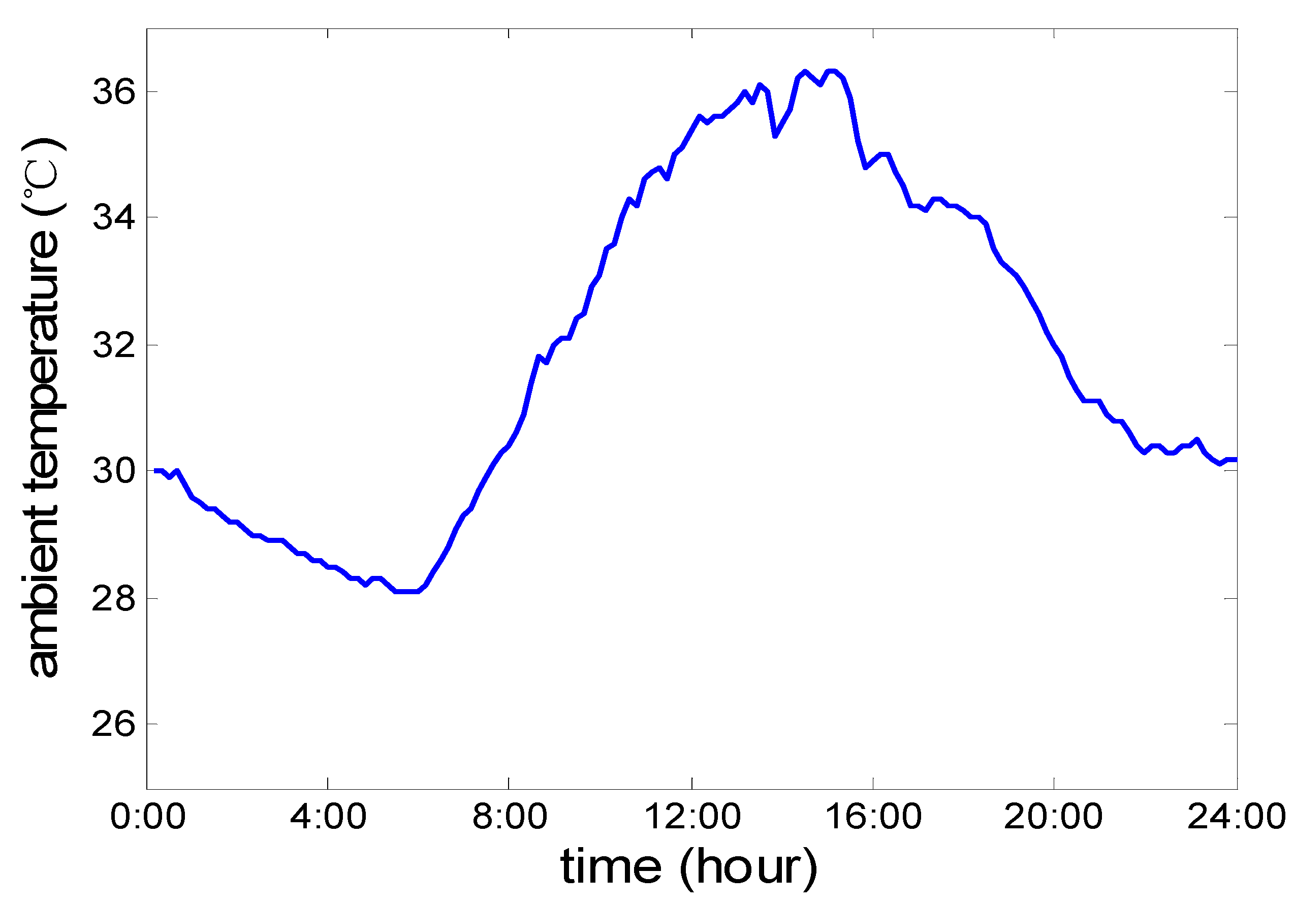
In this scenario, we consider a more realistic situation, which means an ever-changing ambient temperature. We choose 5 August 2014, which was a hot summer day, and the total load was very high. The temperature sensors of the weather station deployed in the area collect practical ambient temperatures once every 10 min. We draw the ambient temperature profile of 24 h as shown in
Figure 18. It is observed that from 12:00 to 15:00, the ambient temperature is high, and the maximum temperature is 36.3 °C.
Figure 18.
Realistic variable ambient temperature.
Figure 18.
Realistic variable ambient temperature.
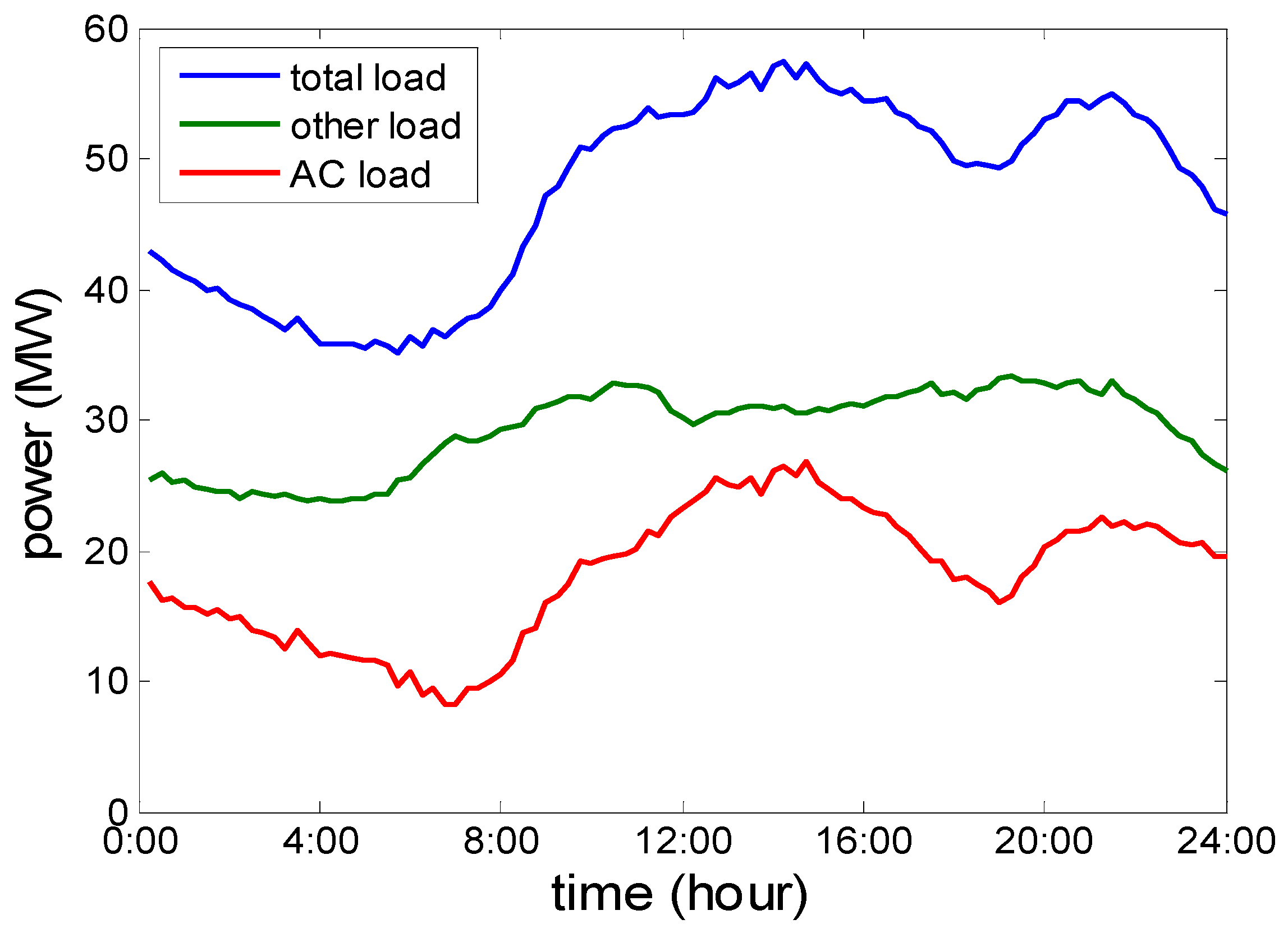
Figure 19 represents 24 h power load of a downtown area in Nanjing, China, where there are 18,000 ACs of 10,000 residents operating on the hot day 5 August 2014. The real data for the load profile, which was collected every 15 min, was provided by State Grid Nanjing power supply company. The real-time temperature on the same day, which was collected every 10 min, was provided by the Jiangsu Provincial Meteorological Bureau. In
Figure 19, the top blue curve is the 96 points load characteristic curve of the customers in the area on the maximum load day. We simulated the load values each second, by using the method of spline interpolation. Peak hours are from 10:30 a.m. to 16:00 p.m. and from 20:00 p.m. to 22:00 p.m. During these periods, the electricity demand outstrips supply, and a power shortfall will appear. As can also be seen, a low load period is from 4:00 a.m. to 8:00 a.m. The maximum load is 5.75 MW and the minimum load is 3.51 MW, and the load peak and off-peak difference is 38.96% of the maximum load. The bottom red curve in
Figure 19 is for the baseline load of 18,000 ACs. The curve is obtained by simulating the two order linear time invariant transfer function model, which is based on the parameters in
Table 1 and the ambient temperature curve in
Figure 19. The total load characteristic curve minus the AC load curve based on the TF model is the green curve of the non-air conditioning load, which is in the middle of the figure.
The population consists of 18,000 ACs. Assuming that at the initial moment, 44.6% of the ACs are on, while the rest of them are off, the whole load control scenario is divided into two stages. The first stage is from 12:00 p.m. to 16:00 p.m., when the grid is in a peak load period. We decide to cut the peak load of ACs to 2 MW. The load aggregator will raise the temperature set point of the ACs to achieve peak load shifting. The second stage takes place between 4:00 a.m. and 8:00 a.m., when the peak load period of the power grid is over, we decide to increase the load of ACs to 1.2 MW to maintain the power consumption of the trough period. The load aggregator will drop the temperature set point of the ACs to realize users’ comfort recovery.
In this scenario, the two order transfer function model of air conditioning is no longer linear time invariant, and instead, it is changing with time. The model parameters vary with the outdoor temperature in the case of equivalent thermal resistance, thermal capacitance and other parameters remaining unchanged.
Figure 19.
24 h power load of a downtown area of Nanjing, China where there are 18,000 ACs of 10,000 residents operating on the hot day 5 August 2014.
Figure 19.
24 h power load of a downtown area of Nanjing, China where there are 18,000 ACs of 10,000 residents operating on the hot day 5 August 2014.
There are two ways to solve this problem. This paper mainly focuses on the load control of ACs to achieve peak load shifting. Since the peak load duration is not long, the first method takes the average of the ambient temperature at intervals of half an hour within the required period of peak load shifting. In less than half an hour, it can be assumed that the ambient temperature is constant. During the period when ACs are participating in demand response, the change of the ambient temperature is not dramatic, especially for the existence of the heat island effect in the city center area. Therefore another method calculates the parameters of the transfer function whenever the outdoor temperature changes 0.5 °C. If the temperature variation is within 0.5 °C, the transfer function of the model is believed to remain unchanged.
In this paper, we adopt the second method. According to the different ambient temperature, the two order transfer function parameters are shown in
Table 4. The numbers in
Table 4 are subsequently calculated by using Equations (21)–(27). The relevant AC parameters used in the calculation can be found in
Table 2. In the process of calculation, the ACs’ other parameters are as follows:
,
and
, all of which remain unchanged.
. The period when ACs could be controlled by the load aggregator is from 4:00 a.m. to 8:00 a.m. and from 12:00 p.m. to 16:00 p.m. Thus, according to the real-time ambient temperature on the warmest day, 5 August 2014, the research scope is identified as (28 °C, 32 °C) and (34 °C, 36 °C).
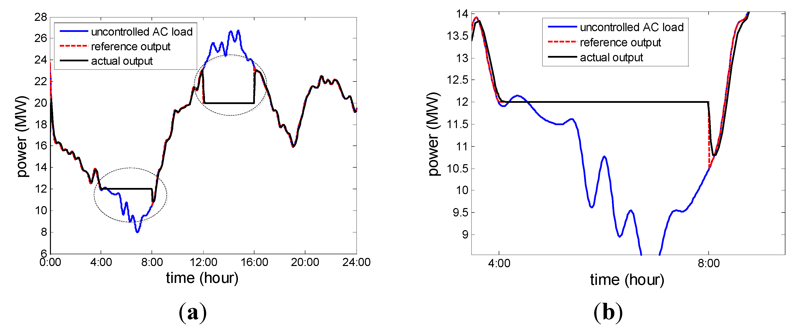
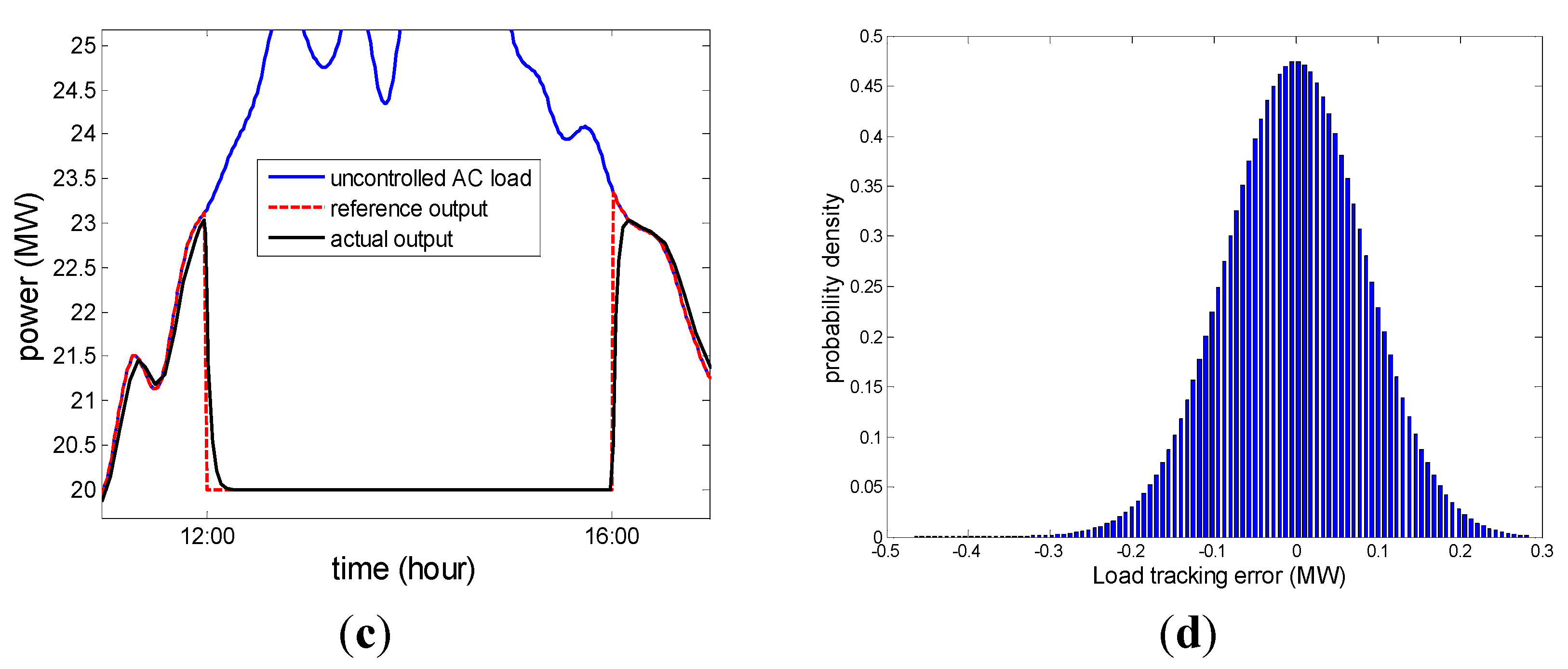
Figure 20 illustrates the effect of the AC load control based on the PSO tuning parameters of the PID controller for load shifting on a hot day when the ambient temperature continues to change. In
Figure 20a, the upper blue curve represents the aggregated power 18,000 ACs without any control, the middle red dashed curve is the desired AC load reference value for load shifting, and the solid black line at the bottom represents the actual output power of AC load based on PSO tuning parameters of the PID controller.
Figure 20b,c is obtained by zooming in on the parts circled by a dotted curve in
Figure 20a. They show the effects of increasing the power output from 4:00 a.m. to 8:00 a.m. and reducing the power output from 12:00 p.m. to 16:00 p.m, respectively.
Figure 20d shows the probability density distribution of the tracking error between the actual output and the reference value.
Table 4.
Parameters of two order transfer function model for ACs.
Table 4.
Parameters of two order transfer function model for ACs.
| Ambient Temperature (°C) | Dss(θ) | r | ξ | ωn | b0 | b1 | b2 |
|---|
| 28 | 0.285 | 0.431 | 0.259 | 0.022 | 0.168 | 0.007 | 0.285 |
| 28.5 | 0.303 | 0.431 | 0.259 | 0.023 | 0.190 | 0.007 | 0.303 |
| 29 | 0.321 | 0.431 | 0.259 | 0.024 | 0.213 | 0.008 | 0.321 |
| 29.5 | 0.339 | 0.431 | 0.259 | 0.026 | 0.237 | 0.008 | 0.339 |
| 30 | 0.357 | 0.431 | 0.259 | 0.027 | 0.263 | 0.009 | 0.357 |
| 30.5 | 0.375 | 0.431 | 0.259 | 0.028 | 0.290 | 0.010 | 0.375 |
| 31 | 0.393 | 0.431 | 0.259 | 0.030 | 0.318 | 0.011 | 0.393 |
| 31.5 | 0.411 | 0.431 | 0.259 | 0.031 | 0.347 | 0.011 | 0.411 |
| 32 | 0.429 | 0.431 | 0.259 | 0.033 | 0.378 | 0.012 | 0.429 |
| 34 | 0.500 | 0.431 | 0.259 | 0.038 | 0.515 | 0.016 | 0.500 |
| 34.5 | 0.518 | 0.431 | 0.259 | 0.039 | 0.552 | 0.017 | 0.518 |
| 35 | 0.536 | 0.431 | 0.259 | 0.041 | 0.591 | 0.018 | 0.536 |
| 35.5 | 0.554 | 0.431 | 0.259 | 0.042 | 0.631 | 0.019 | 0.554 |
| 36 | 0.571 | 0.431 | 0.259 | 0.043 | 0.672 | 0.019 | 0.571 |
Based on the discussions above, one can draw the conclusion that through the PID controller based on the PSO algorithm, the output power of 18,000 ACs can be controlled by adjusting the temperature set point offset. Throughout the control period, the output power of the air conditionings has been following the reference value closely, and the tracking error is small. During peak hours, the load aggregator can reduce the power of ACs by up to 6 MW, and maintain the total load of n ACs at about 20 MW. To some extent, the power shortage has been eased. In peak-off hours, the load aggregator can increase the power of ACs by 4 MW to make the load curve smoother, and maintain the total load of n ACs at about 12 MW.
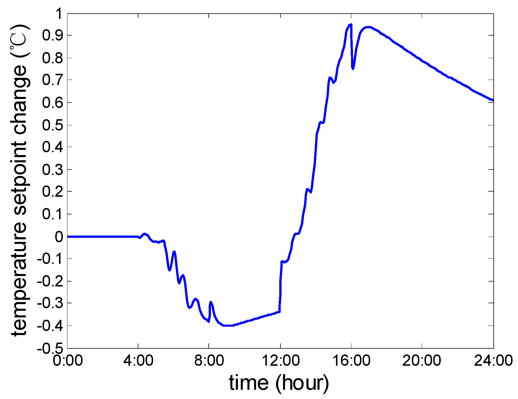
Figure 21 shows the variation of ACs’ temperature set point offset, which is also the control signal of the two order transfer function model for the air conditioning group. The range of air conditioning set point temperature is [−0.4 °C, 0.95 °C].
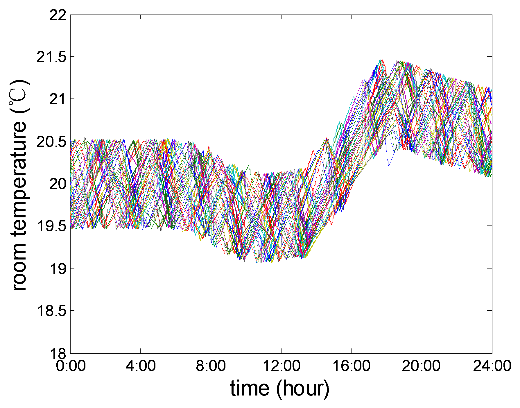
Figure 22 shows the variation of the indoor temperature of 30 random ACs. The hysteresis width of the room temperature, which varies with the air conditioning temperature set point
u(
t), has remained unchanged
H = 1 °C. The figure illustrates such a process: the ACs’ temperature set point can be controlled by the load aggregator who sets a higher value to reduce the load as well as setting a lower value to increase the load. The variation range of the indoor temperature is [19.1 °C, 21.4 °C]. Therefore, load control can be achieved without affecting human comfort level.
Figure 20.
(a), (b), (c) A comparison between the aggregated power of 18,000 ACs without any control, the desired AC load reference value for load shifting, and the actual output power of AC load based on PSO tuning parameters of the PID controller. (d) Probability density distribution of the tracking error between the actual output power and the reference value. The model is simulated for a hot day, and the ambient temperature continues to change.
At 16:00, when the load control period is over, the temperature set point offset does not return to 0. Instead, it continues changing (in
Figure 21) and the room temperature does not directly return to the initial value [19.5 °C, 20.5 °C] (in
Figure 22). The reason for this phenomenon is that, within the short time for the air-conditioning chillers to restart after shutdown, the power demand is usually significantly higher. This is the pattern of the air conditioning which makes the load rebound before and after the load control event. In order to bring the load curve back to the state before controlling, such as the curve after 16:00 p.m. in
Figure 20a, a continuous control is required for some time after the load management.
Figure 21.
The variation of ACs’ temperature set point offset.
Figure 21.
The variation of ACs’ temperature set point offset.
Figure 22.
The variation of the indoor temperature of 30 random ACs.
Figure 22.
The variation of the indoor temperature of 30 random ACs.
The novelty provided in this section is as follows: in the variable ambient temperature scenario, the two order transfer function model of air conditioning is no longer linear time invariant, and instead it changes over time. The model parameters vary with the outdoor temperature. This paper puts forward two suggestions to solve this problem, and we adopt the second one.


