
Magnetic Field Equivalent Current Analysis-Based Radial Force Control for Bearingless Permanent Magnet Synchronous Motors

Abstract
:1. Introduction
2. Magnetic Field Equivalent Current-Based Analysis of Radial Suspension Forces
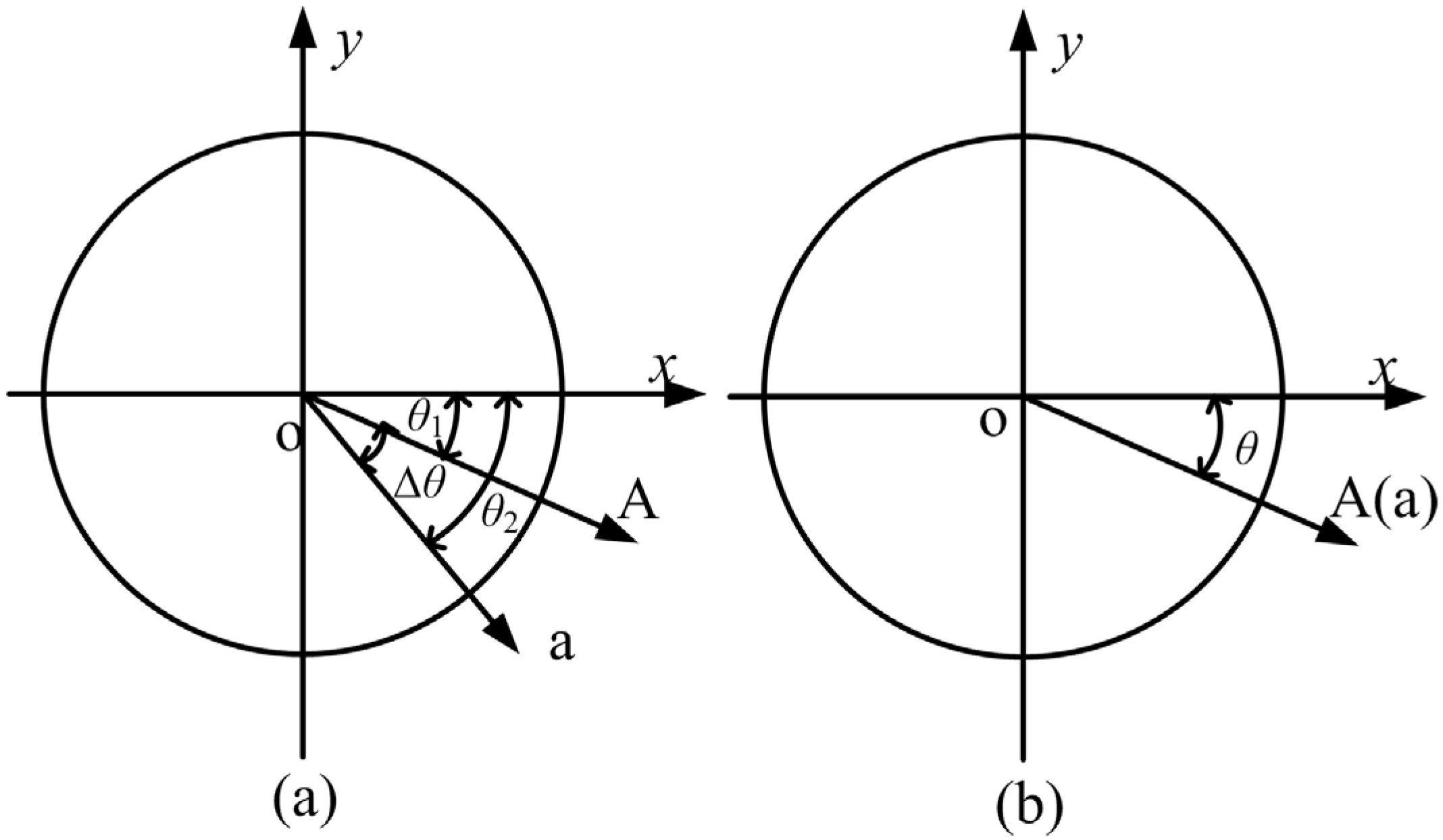
2.1. Fundamental Theory of the Magnetic Field Equivalent Current Analysis Method


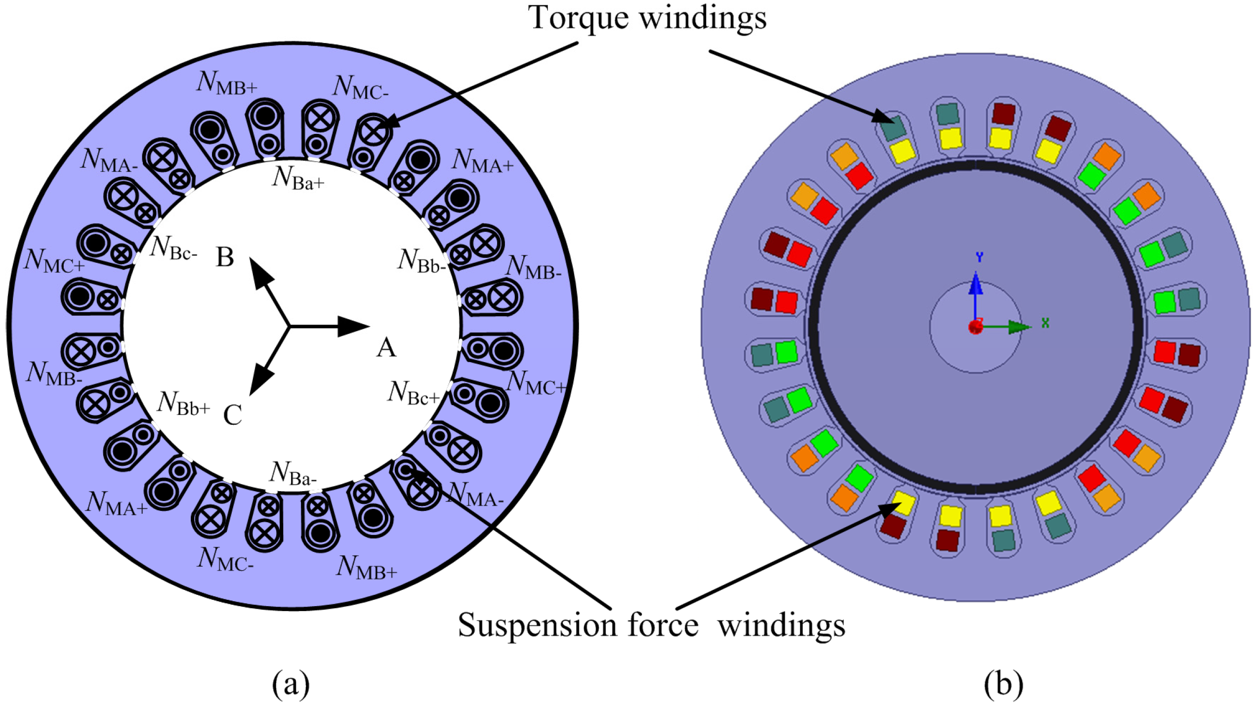
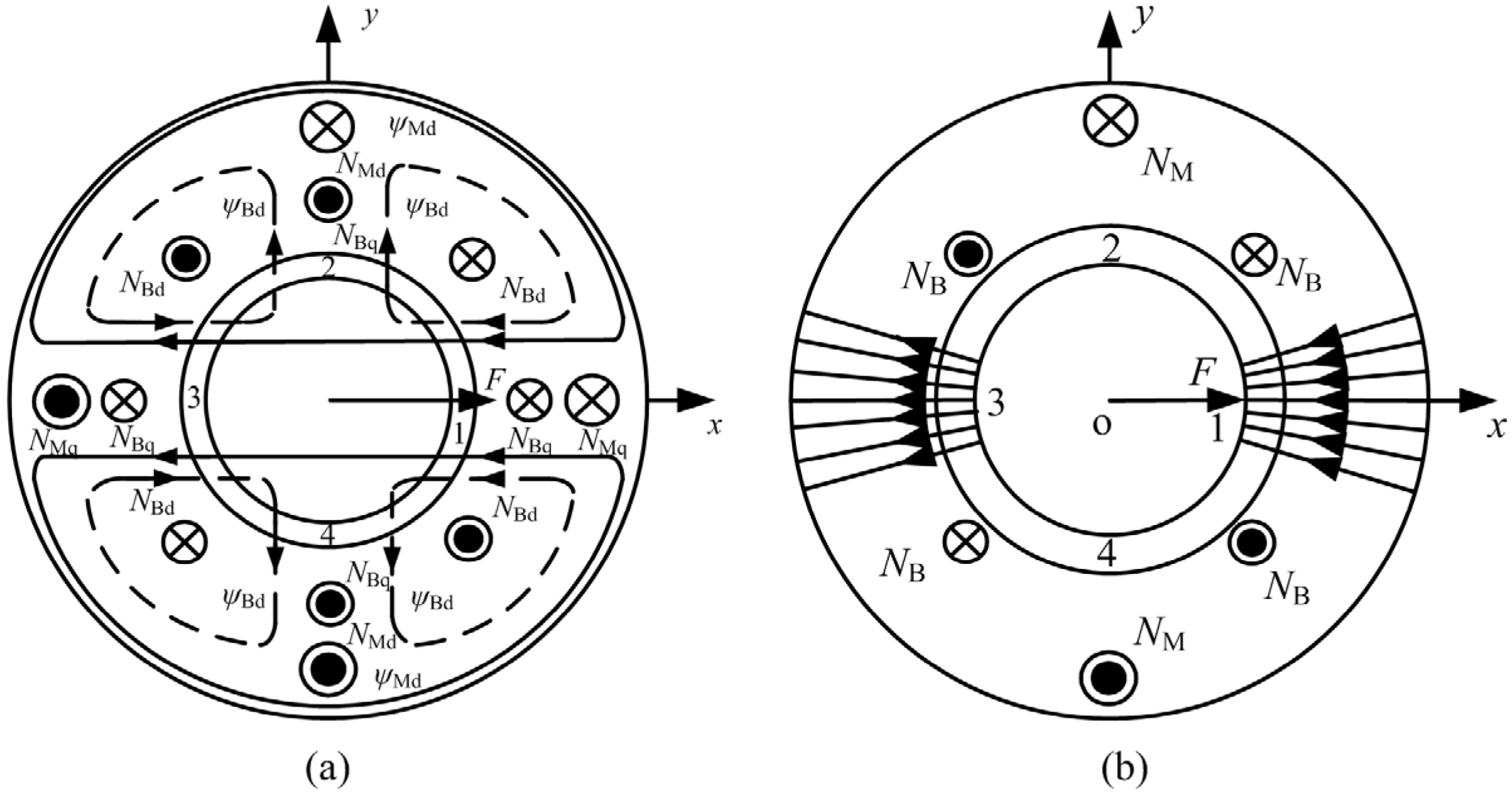
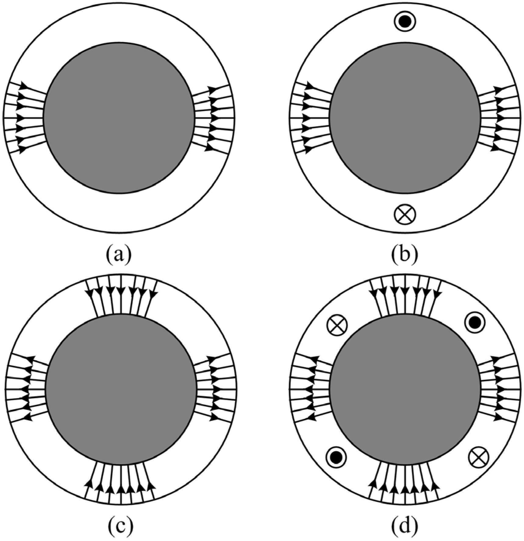
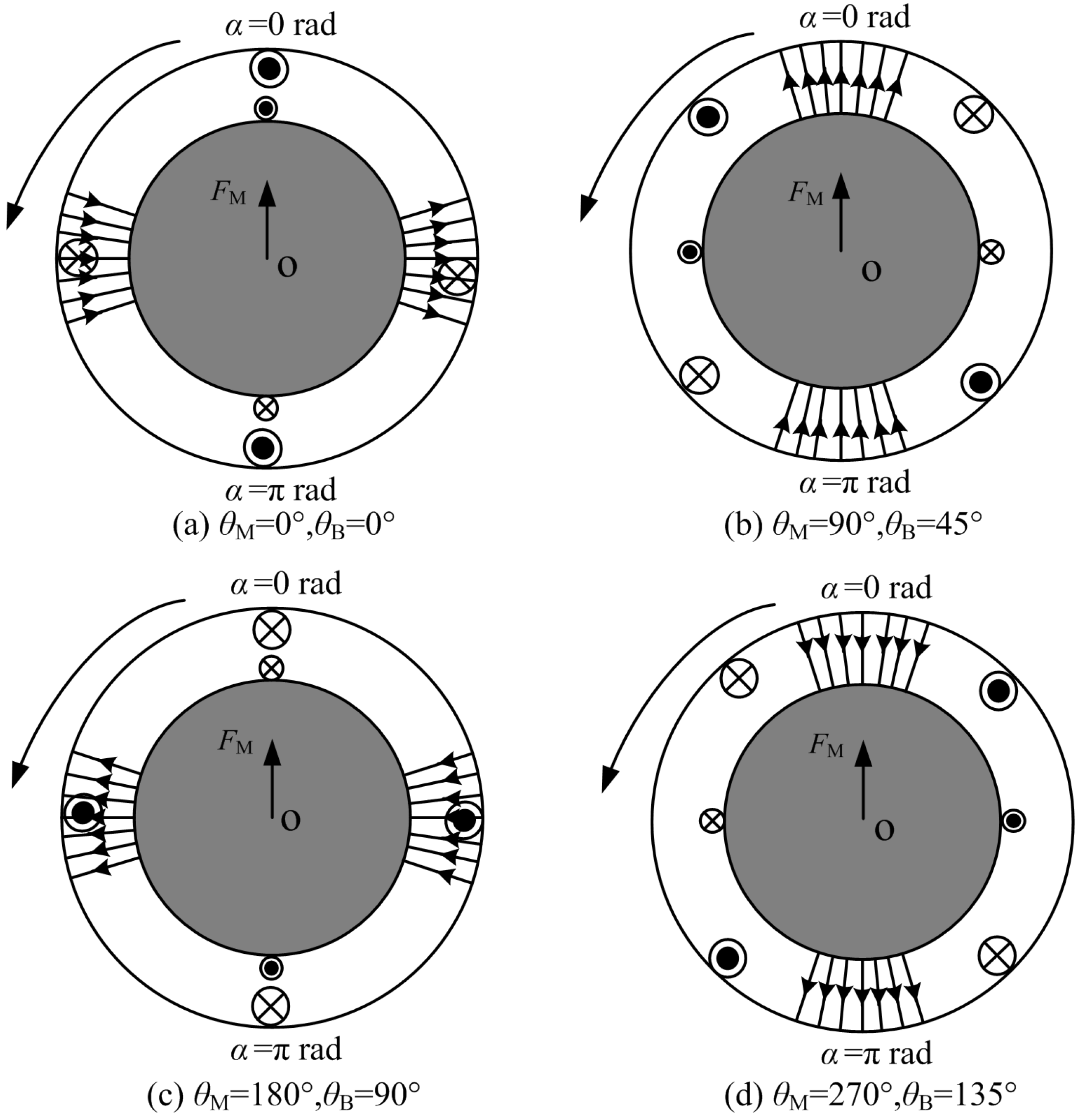
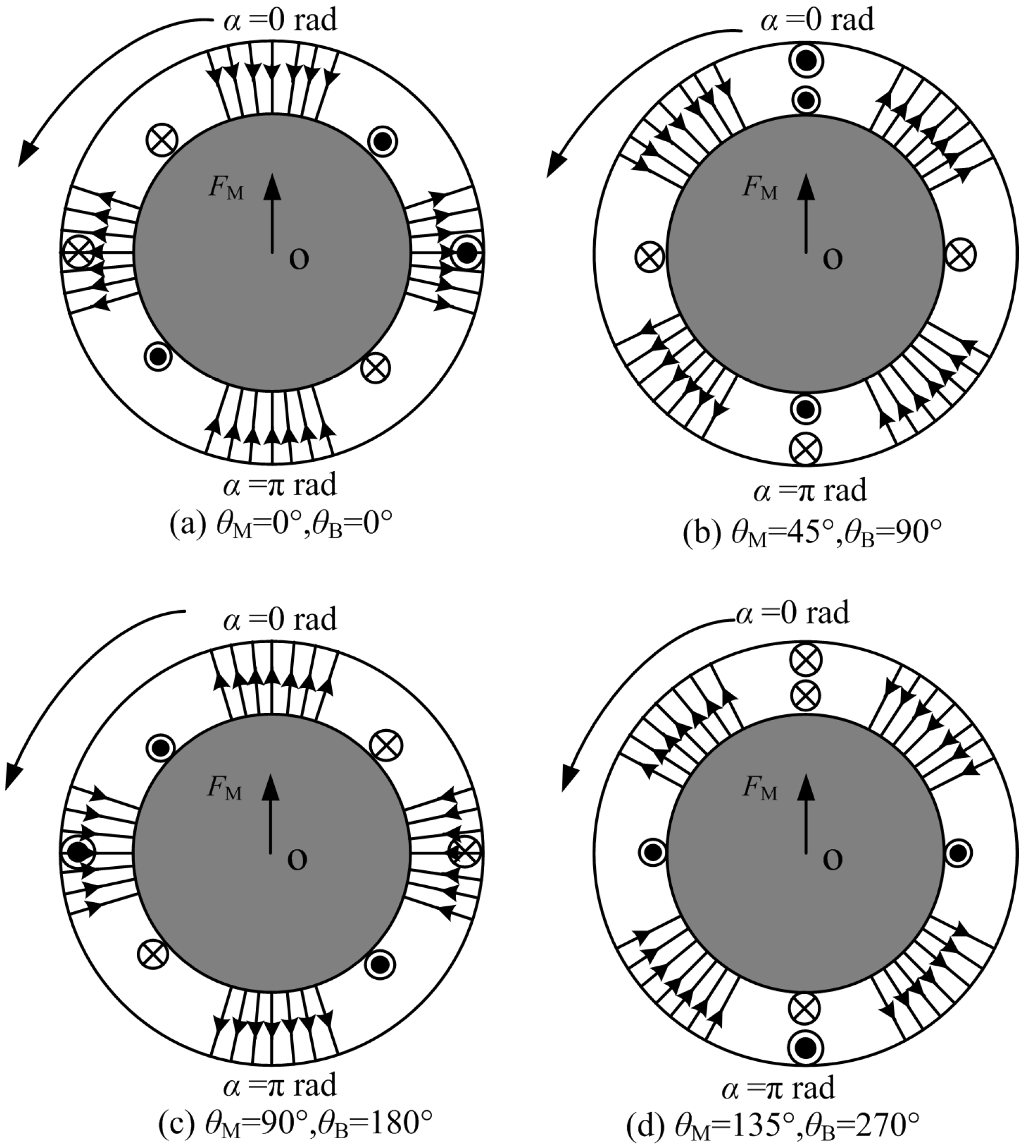
2.2. The Principle of Radial Suspension Force Generation for the BPMSM
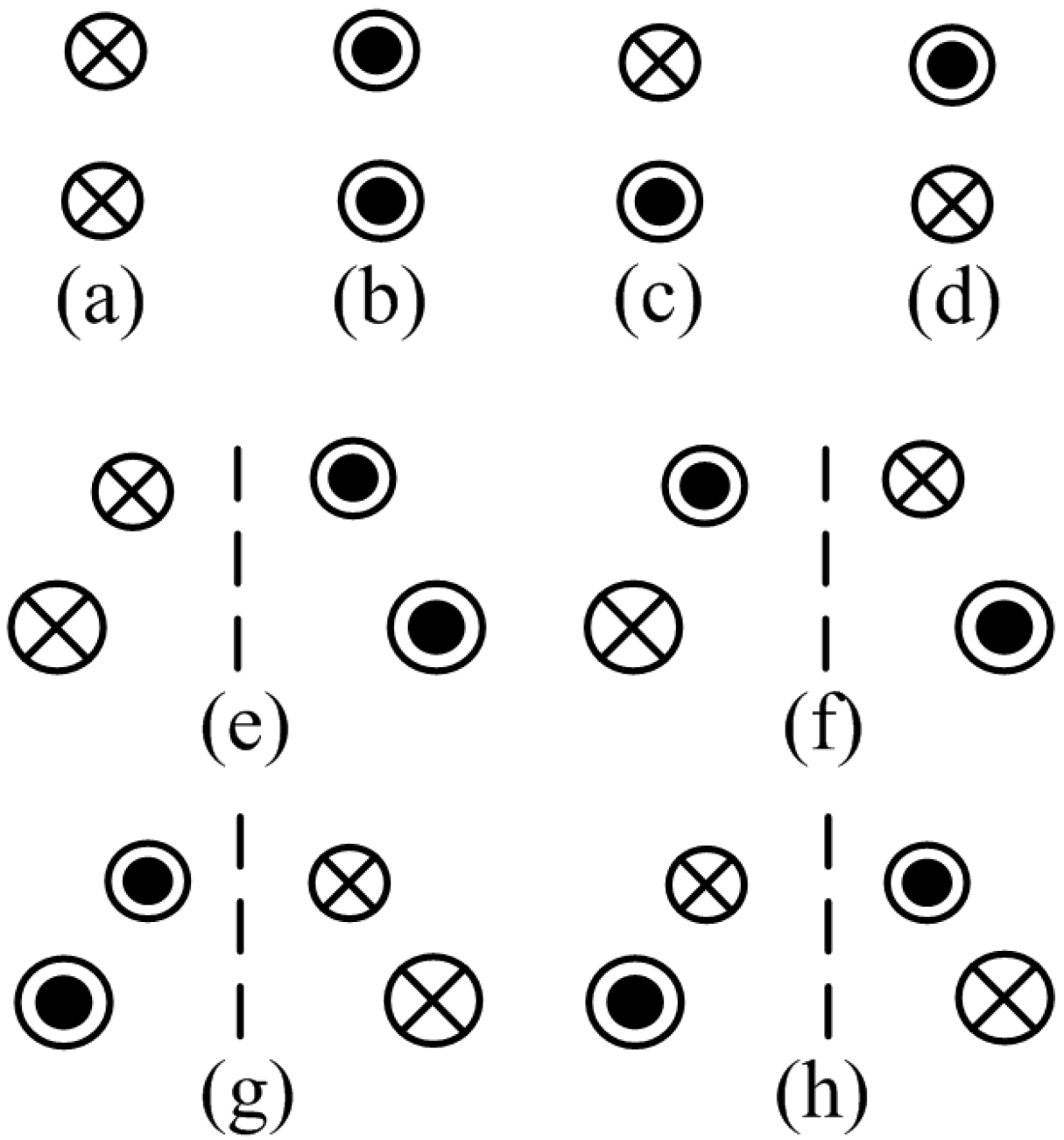
3. Analysis on Producing Stable Radial Suspension Force for the BPMSM


4. Mathematical Model of Radial Suspension Force for the BPMSM
4.1. Analytical Model of Radial Suspension Force for the BPMSM
4.2. Analytical Model of Electromagnetic Torque for the BPMSM
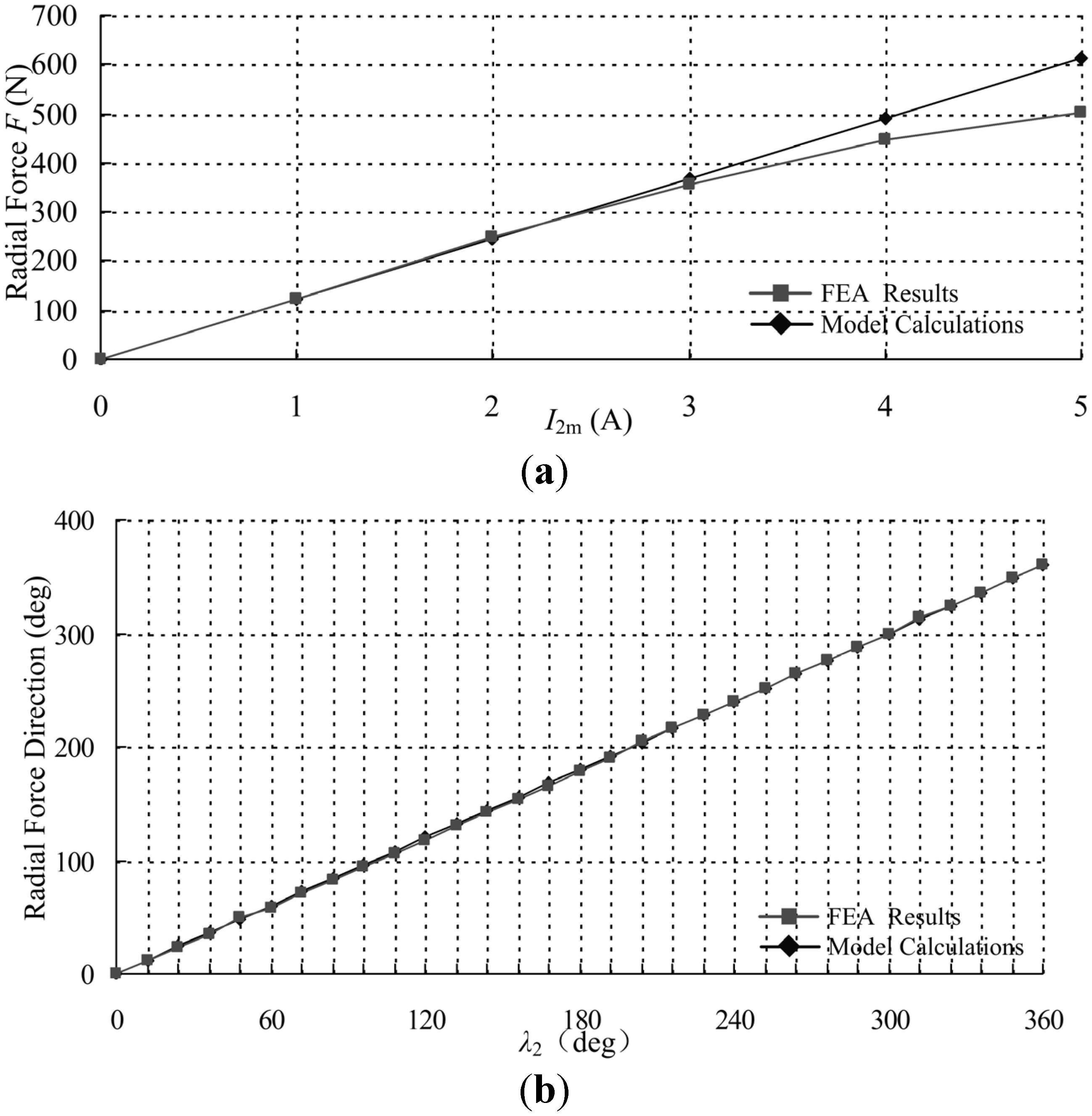
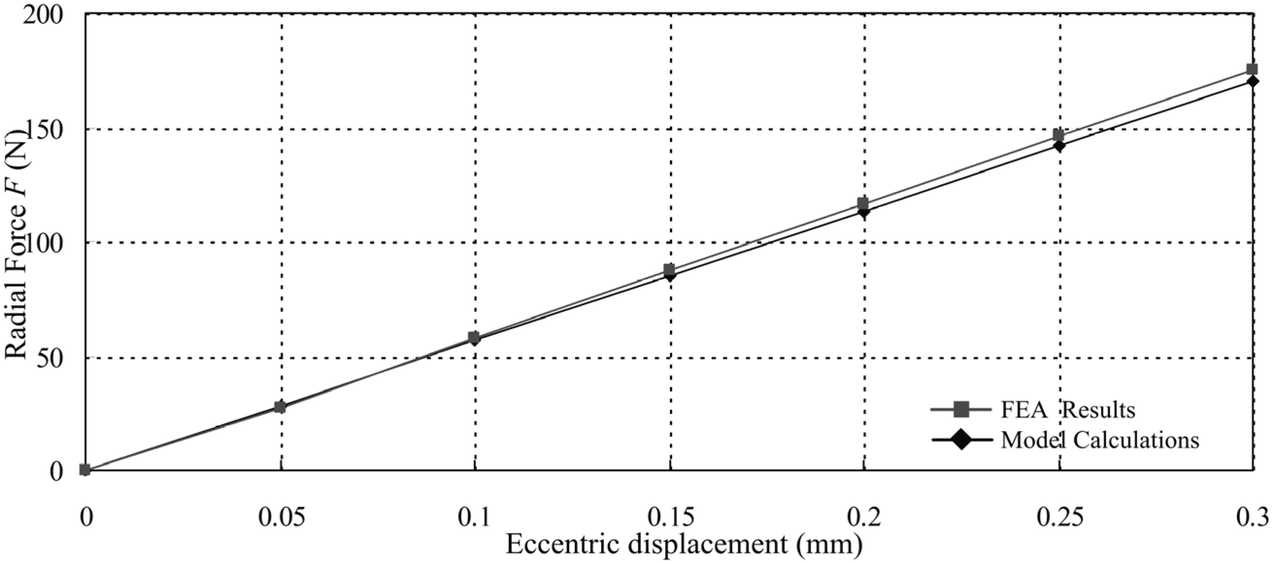
4.3. FEA Validation of the Model

| Parameter | Symbol | Vaule |
|---|---|---|
| Motor unit geometry and torque system data | ||
| Rated mechanical power | PN | 500 W |
| Stator slot count | Q | 24 |
| Stator inner diameter | dsi | 75 mm |
| Stator outer diameter | dso | 120 mm |
| Rotor outer diameter | dro | 73 mm |
| Auxiliary bearing thickness | ha | 0.7 mm |
| Pole pair count | PM | 1 |
| Torque winding wire diameter | Ф | 0.71 mm |
| Turns of torque winding per one slot | NM | 22 |
| Stacking coefficient | ks | 0.95 |
| Number of winding parallel ways | aM | 1 |
| Winding connection | Y | - |
| Mechanical air gap length | g | 1 mm |
| Permanent magnetic material | - | NdFeB |
| Coercive force | Hc | −890 kA/m |
| Magnet thickness | hm | 2 mm |
| Magnet remanence at 20°C | Br | 1.1 T |
| Suspension force system data | ||
| Pole pair count | PB | 2 |
| Turns of suspension force winding per one slot | NB | 22 |
| Number of winding parallel ways | aB | 1 |
| Winding connection | Y | - |
| Force/current coefficient | km | 122.325 N/A |
| Force/displacement coefficient | kecc | 568.02 N/mm |

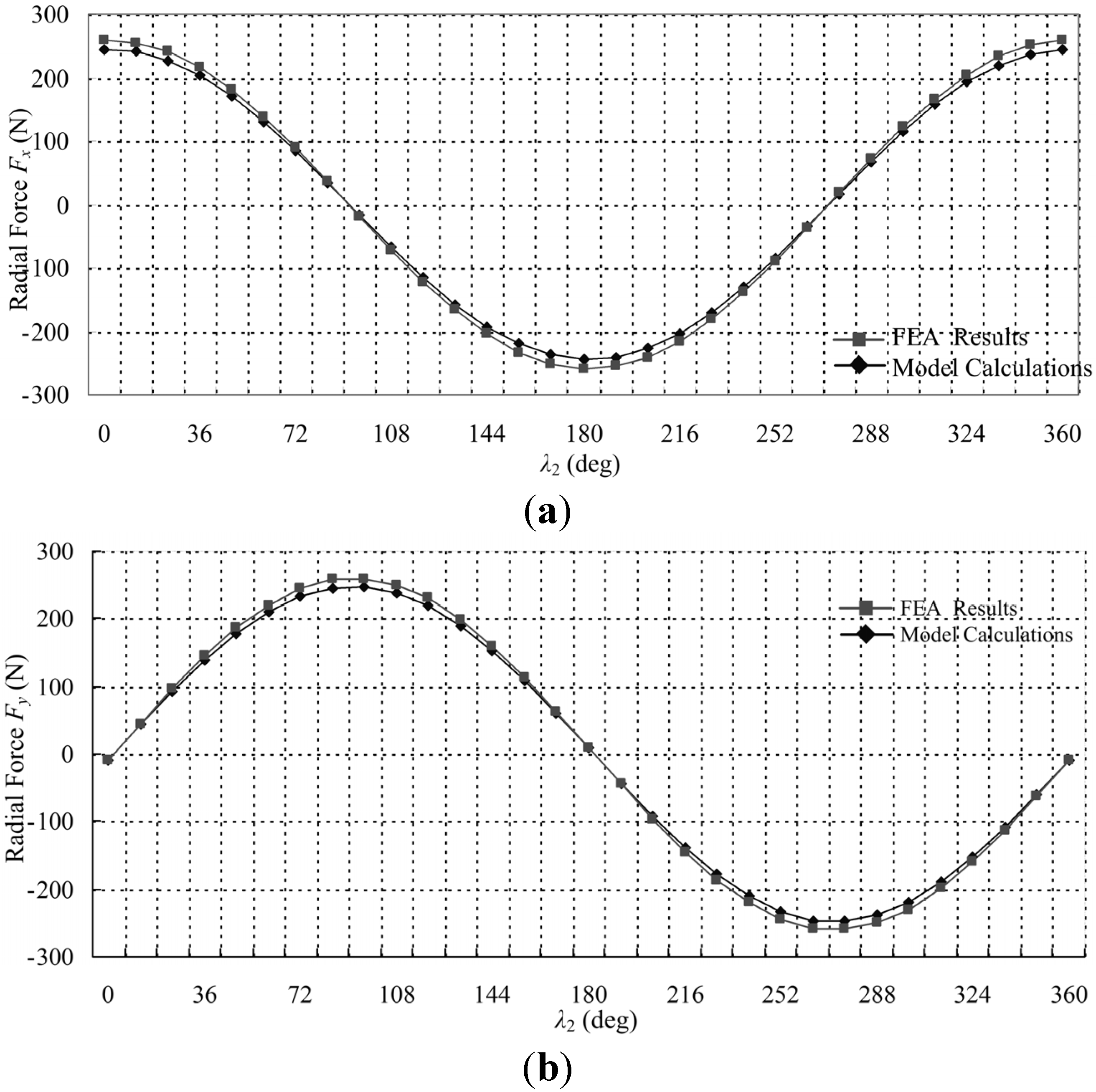

| IBm (A) | The FEA results (N) | Mathematical model values (N) | Error |
|---|---|---|---|
| 1 | 123.5032 | 122.325 | 0.96% |
| 2 | 247.6507 | 244.65 | 1.23% |
| 3 | 365.9582 | 366.975 | 2.73% |
| 4 | 448.0844 | 489.3 | 8.42% |
| 5 | 501.6163 | 611.625 | 17.99% |
| Eccentric displacement (mm) | The FEA results (N) | Mathematical model values (N) | Error |
|---|---|---|---|
| 0.1 | 28.4 | 27.34 | 1.99% |
| 0.2 | 113.604 | 116.462 | 2.51% |
| 0.3 | 170.46 | 174.953 | 2.67% |
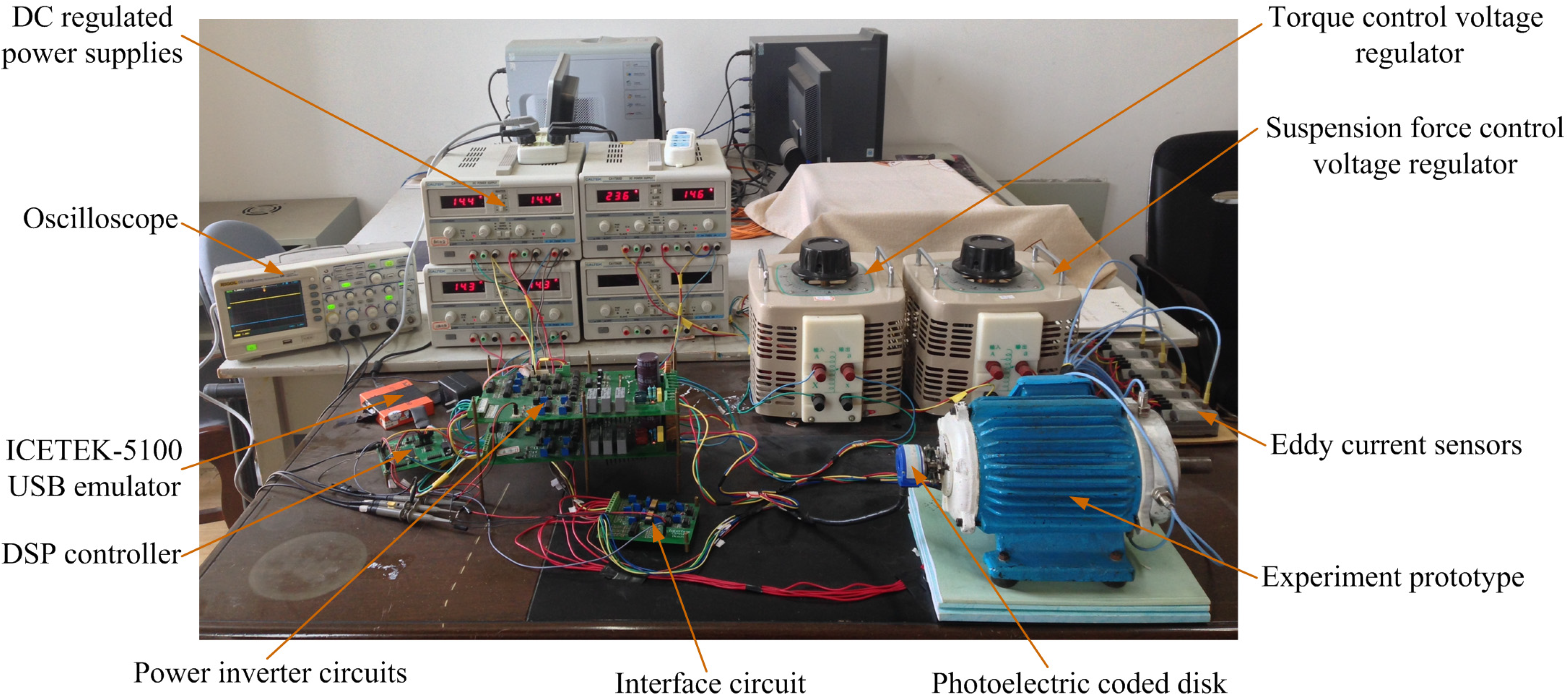
5. Experimental System for the BPMSM
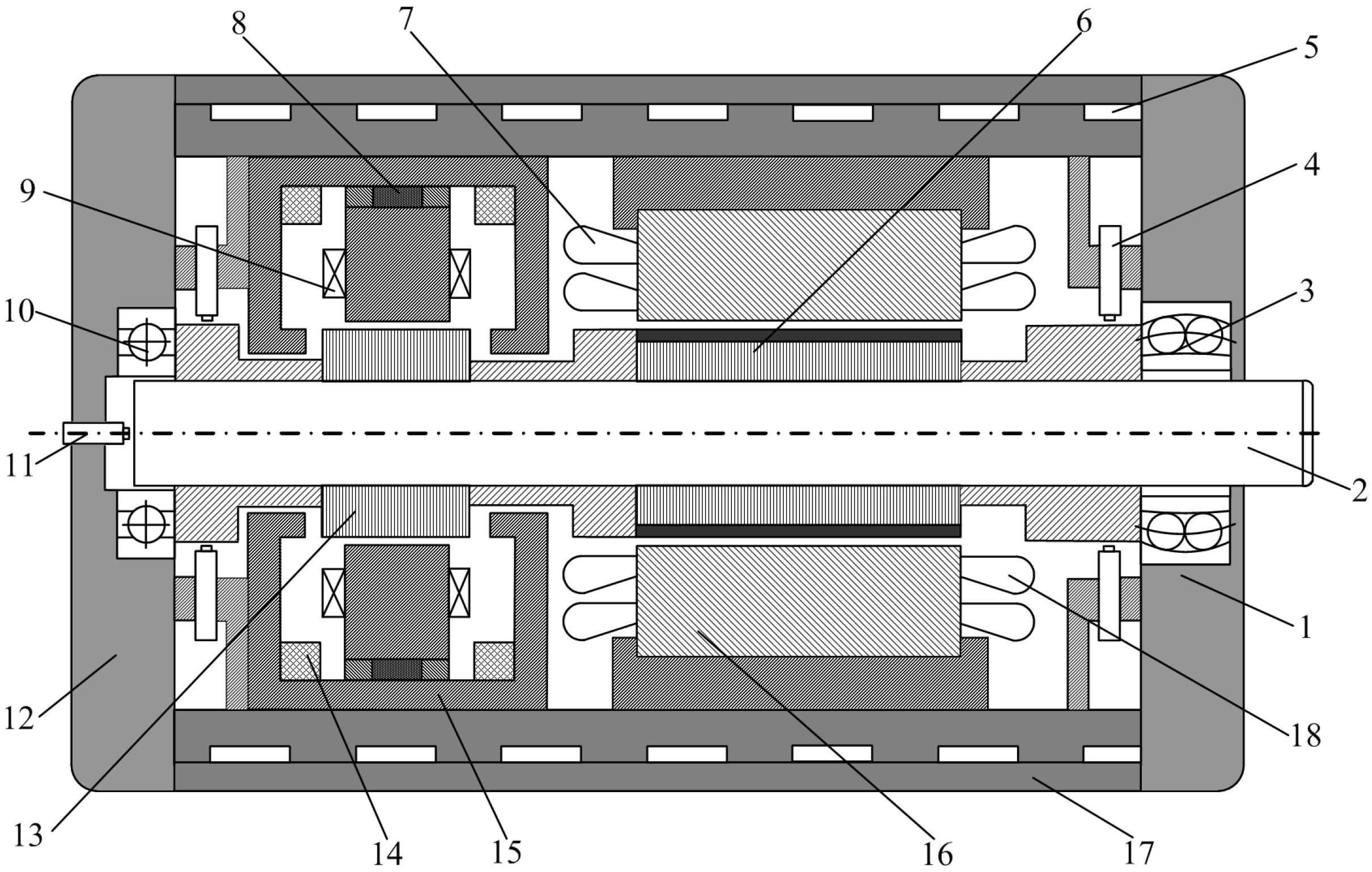
5.1. Prototype Machine Structure

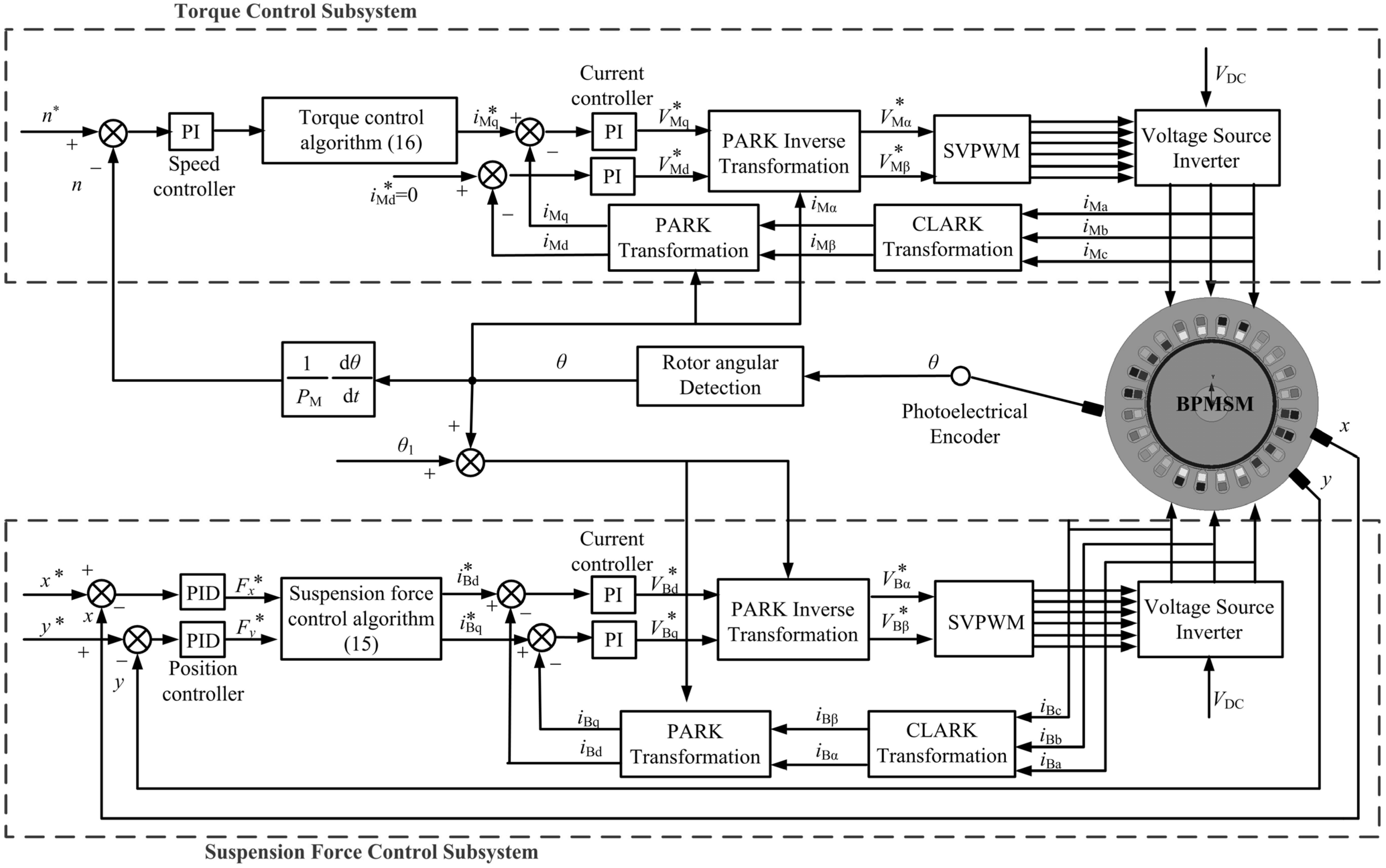
5.2. Control of Torque and Radial Suspension Force for the BPMSM

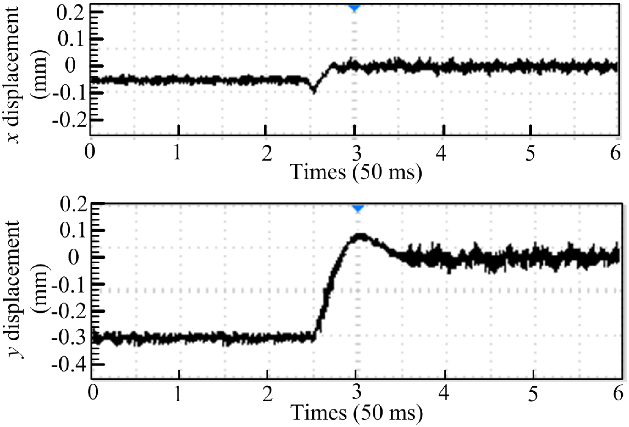
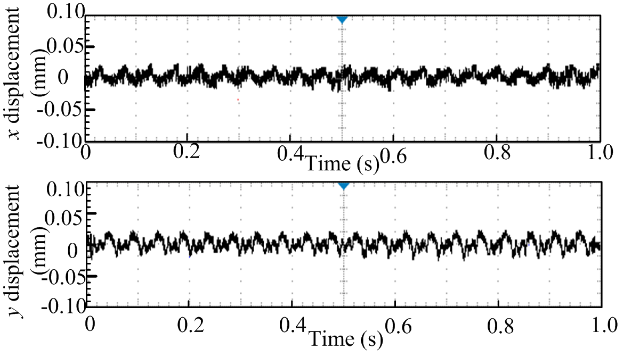
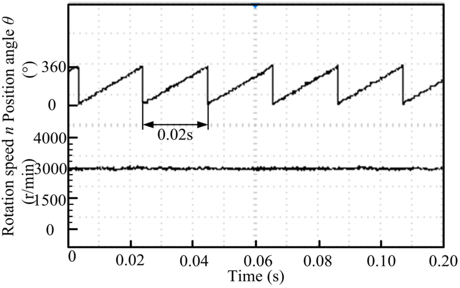
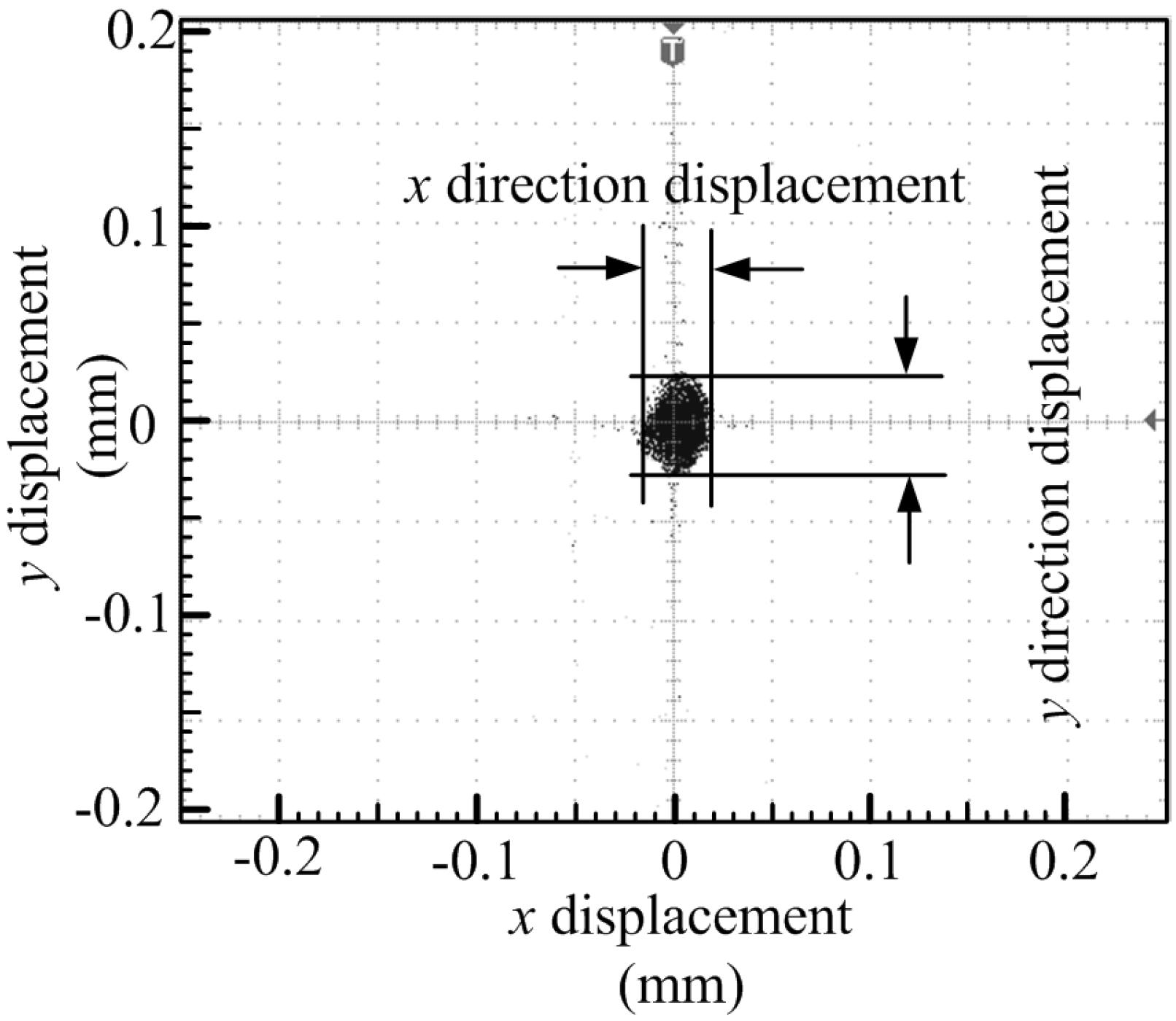
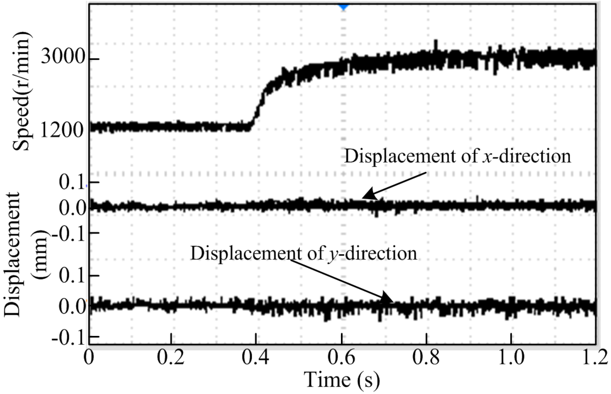
6. Analysis on Experimental


7. Conclusions
Acknowledgments
Author Contributions
Conflicts of Interest
References
- Baumgartner, T.; Burkart, R.M.; Kolar, J. Analysis and Design of a 300-W 500 000-r/min Slotless Self-Bearing Permanent-Magnet Motor. IEEE Trans. Ind. Electron. 2014, 61, 4326–4336. [Google Scholar] [CrossRef]
- Nguyen, Q.D.; Ueno, S. Modeling and control of Salient-Pole Permanent Magnet Axial-Gap Self-Bearing Motor. IEEE Trans. Mechatron. 2011, 16, 516–528. [Google Scholar] [CrossRef]
- Qiu, Z.J.; Deng, Z.Q.; Wang, X.L.; Meng, X.L. Study on the Modeling and Control of a Permanent-magnet-type Bearingless Motor Considering Rotor Eccentricity and Lorenz Force. Proc. Chin. Soc. Electr. Eng. 2007, 27, 64–70. [Google Scholar]
- Zhu, H.Q.; Cheng, Q.L.; Wang, C.B. Modeling of bearingless permanent magnet synchronous motor based on mechanical to electrical coordinates transformation. Sci. China Ser. E 2009, 52, 3736–3744. [Google Scholar] [CrossRef]
- Ooshima, M.; Miyazawa, S.; Chiba, A.; Nakamura, F.; Fukao, T. A rotor design of a permanent magnet-type bearingless motor considering demagnetization. In Proceedings of the Power Conversation, Nagaoka, Japan, 3–6 August 1997; pp. 655–660.
- Sun, X.D.; Zhu, H.Q.; Zhang, T. Nonlinear decoupling control for 5 degrees-of-freedom bearingless permanent magnet synchronous motor. In Proceedings of the Power Electronics and Motion Control Conference, Wuhan, China, 17–20 May 2009.
- Kascak, P.; Jansen, R.; Dever, T.; Loparo, K.; Nahorny, A. Motoring performance of a conical pole-pair separated bearingless electric machine. In Energyteck; IEEE: New York, NY, USA, 2011; pp. 1–6. [Google Scholar]
- Zhang, S.; Luo, F.L. Direct control of radial displacement for bearingless permanent-magnet-type synchronous motors. IEEE Trans. Ind. Electron. 2009, 56, 542–552. [Google Scholar] [CrossRef]
- Sun, X.D.; Zhu, H.Q.; Zhang, T. Sliding mode variable structure control for radial suspension forces of bearingless permanent magnet synchronous motor based on inverse system method. In Proceedings of the Power Electronic and Motion Control Conference, Wuhan, China, 17–20 May 2009.
- Sun, X.D.; Zhu, H.Q.; Pan, W. Decoupling control of bearingless permanent magnet-type synchronous motor using artificial neural networks-based inverse system method. Int. J. Model. Ident. Control 2009, 8, 114–121. [Google Scholar] [CrossRef]
- Khoo, W.K.S. Bridge configured winding for polyphase self-bearing machines. IEEE Trans. Magn. 2005, 41, 1289–1295. [Google Scholar] [CrossRef]
- Zhang, S.R.; Luo, F.L. Direct Control of Radial Displacement for Bearingless Permanent-Magnet-Type Synchronous Motors. IEEE Trans. Ind. Electron. 2009, 56, 542–552. [Google Scholar] [CrossRef]
- Amrhein, W.; Silber, S.; Nenninger, K. Levitation forces in bearingless permanent magnet motors. IEEE Trans. Magn. 1999, 35, 4052–4054. [Google Scholar] [CrossRef]
- Chiba, A.; Fukao, T.; Ichikawa, O.; Oshima, M.; Takemoto, M.; Dorrell, D.G. Magnetic Bearings and Bearingless Drives; Elserver: Amsterdam, The Netherland, 2005; p. 400. [Google Scholar]
- Chiba, A.; Hanazawa, M.; Fukao, T.; Rahman, M.A. Effects of magnetic saturation on radial suspension force of bearingless synchronous reluctance motors. IEEE Trans. Ind. Appl. 1996, 32, 354–362. [Google Scholar] [CrossRef]
- Li, H.; Zhu, H.Q. Bearingless motor’s radial suspension force control based on virtual winding current analysis. In Proceedings of the Electrical Machines and Systems (ICEMS), Hangzhou, China, 22–25 October 2014; pp. 2141–2146.
- Pillay, P.; Krishnan, R. Modeling of permanent magnet motor drives. IEEE Trans. Ind. Election. 2002, 35, 537–541. [Google Scholar] [CrossRef]
- Sun, X.D.; Chen, L.; Yang, Z.B.; Zhu, H.Q.; Zuo, W.Q.; Shi, K. Modeling of a Bearingless Permanent Magnet Synchronous Motor Considering Rotor Eccentricity and Coupling Relationship of Windings. Trans. CES 2013, 28, 63–70. [Google Scholar]
- Zhu, H.Q.; Wei, J. Radial suspension force modeling on interior bearingless permanent magnet synchronous motors. Electr. Mach. Control 2013, 5, 45–50. [Google Scholar]
- Zhu, H.Q.; Wu, L.; Li, T.H.; Sun, Y.K. Suspension principle of rotor and decoupling control for bearingless permanent magnet-type synchronous motors. J. Southeast Univ. (Nat. Sci. Edit.) 2005, 35, 34–38. [Google Scholar]
- Inagaki, K.; Chiba, A.; Rahman, M.A.; Fukao, T. Performance characteristics of inset-type permanent magnet bearingless motor drives. In Proceedings of the Power Engineering Society Winter Meeting, Singapore, 23–27 January 2000; pp. 202–207.
- Deng, Z.Q.; Qiu, Z.J.; Wang, X.L.; Yan, Y.G. Study on rotor flux orientation control of permanent magnet bearingless synchronous motors. Proc. Chin. Soc. Electr. Eng. 2005, 25, 48–52. [Google Scholar]
- Munteanu, G.; Binder, A.; Schneider, T.; Funieru, B. No-load tests of a 40 kW high-speed bearingless permanent magnet synchronous motor. In Proceedings of the 2010 International Symposium on Power Electronics Electrical Drives Automation and Motion (SPEEDAM), Pisa, Italy, 14–16 June 2010; IEEE: New York, NY, USA; pp. 1460–1465.
- Yajima, S.; Takemoto, M.; Tanaka, Y.; Chiba, A.; Tadashi, F. Total efficiency of a deeply buried permanent magnet type bearingless motor equipped with 2-pole motor windings and 4-pole suspension windings. In Proceedings of the Power Engineering Society General Meeting, Tampa, FL, USA, 24–28 June 2007; IEEE: New York, NY, USA; pp. 1–7.
© 2015 by the authors; licensee MDPI, Basel, Switzerland. This article is an open access article distributed under the terms and conditions of the Creative Commons Attribution license (http://creativecommons.org/licenses/by/4.0/).
Share and Cite
Zhu, H.; Li, H. Magnetic Field Equivalent Current Analysis-Based Radial Force Control for Bearingless Permanent Magnet Synchronous Motors. Energies 2015, 8, 4920-4942. https://doi.org/10.3390/en8064920
Zhu H, Li H. Magnetic Field Equivalent Current Analysis-Based Radial Force Control for Bearingless Permanent Magnet Synchronous Motors. Energies. 2015; 8(6):4920-4942. https://doi.org/10.3390/en8064920
Chicago/Turabian StyleZhu, Huangqiu, and Hui Li. 2015. "Magnetic Field Equivalent Current Analysis-Based Radial Force Control for Bearingless Permanent Magnet Synchronous Motors" Energies 8, no. 6: 4920-4942. https://doi.org/10.3390/en8064920
APA StyleZhu, H., & Li, H. (2015). Magnetic Field Equivalent Current Analysis-Based Radial Force Control for Bearingless Permanent Magnet Synchronous Motors. Energies, 8(6), 4920-4942. https://doi.org/10.3390/en8064920