Optimizing Capacities of Distributed Generation and Energy Storage in a Small Autonomous Power System Considering Uncertainty in Renewables

Abstract

This paper explores real power generation planning, considering distributed generation resources and energy storage in a small standalone power system. On account of the Kyoto Protocol and Copenhagen Accord, wind and photovoltaic (PV) powers are considered as clean and renewable energies. In this study, a genetic algorithm (GA) was used to determine the optimal capacities of wind-turbine-generators, PV, diesel generators and energy storage in a small standalone power system. The investment costs (installation, unit and maintenance costs) of the distributed generation resources and energy storage and the cost of fuel for the diesel generators were minimized while the reliability requirement and CO₂ emission limit were fulfilled. The renewable sources and loads were modeled by random variables because of their uncertainties. The equality and inequality constraints in the genetic algorithms were treated by cumulant effects and cumulative probability of random variables, respectively. The IEEE reliability data for an 8760 h load profile with a 150 kW peak load were used to demonstrate the applicability of the proposed method.

1. Introduction

Small standalone power systems are found on offshore islands and indigenous areas in mountains. This paper addresses the generation expansion planning involving wind-turbine generators (WTG), photovoltaic (PV), diesel generators, and energy storage (ES) for small standalone power systems to meet the restriction of fuel emissions [1,2]. Many works have addressed the generation expansion planning in small standalone power systems [3,4,5,6,7,8,9,10,11,12,13,14,15,16,17,18,19]. Existing methodologies fall into three categories: reliability, optimization-, and enumeration-based methods. With respect to reliability-based methods, Billinton presented a methodology for sizing the WTG and PV array, considering investment cost, loss of power supply probability (LPSP) and loss of load probability (LOLP) [3]. Ai compared the optimal sizes of a WTG/PV hybrid system with the annual LPSP values [4]. Nelson proposed a method using system load matching and LPSP, in which the number of WTGs was treated as an independent variable and the number of PV arrays was treated as a dependent variable [5]. Diaf considered different types and capacities of renewable sources to yield the desired reliability indices using the smallest “levelized cost of energy” [6].

Optimization-based methods were originally developed to reduce the investment, operating and fuel costs of distributed generation resources [7,8,9,10,11,12,13,14,15,16]. Katsigiannis combined simulated annealing and tabu search to solve the optimal capacities of WTG and PV in small autonomous power systems [7]. Vrettos and Papathanassiou investigated the capacity of the hybrid system components (diesel, WTG, and ES) by conducting a parametric analysis and then optimized the values using genetic algorithms [8]. Belfkira used the DIviding RECTangles (DIRECT) algorithm to optimize the number and types of components of the hybrid system, ensuring that the total cost of the system was minimized and that the system demand was completely covered [9]. Cabral et al. minimized both costs of PV arrays and energy storage system while considering reliability constraints and uncertain irradiation levels [10]. Lujano-Rojas et al. employed artificial neural networks to acquire the expected values of net present cost (NPC) and reliability and used genetic algorithms to minimize the operational cost of the system [11]. The probability of a determined level of reliability must be guaranteed in a certain grade. Lujano-Rojas et al. optimized both the NPC and the energy index of unreliability [12]. NPC is the cost throughout the operative lifetime of the system, comprising the annualized capital cost and the annualized replacement cost. Kaviani et al. in [13] and Chen in [14] minimized the system costs involving investment, replacement, and operation and maintenance plus loss of load costs using particle swarm optimization (PSO). Borhanazad et al. minimized the sum of weighted cost and reliability index to balance the cost-effectiveness of the system and the quality of service in a microgrid using PSO [15]. Sharafi and ELMekkawy optimized the cost, reliability and fuel emission simultaneously using ε-constrained PSO [16].

Apart from reliability- and optimization-based methods, the enumeration method was designed to compare different types and sizes of distributed generation units in terms of investment, operation and fuel costs. Diaf et al. estimated the appropriate dimensions of a stand-alone hybrid PV/wind system that guaranteed the energy autonomy of a typical remote consumer with the lowest levelized cost of energy (LCE) [17]. Kaldellis assessed the smallest capacity of the wind turbine using its nominal power, capacity factor and mean power coefficient [18]. Recently, Luna-Rubio et al. briefly reviewed sizing methodologies and hybrid energy metrics (such as reliability and net present value) that have been developed in recent years [19].

The above works have the following limitations:

(a)

Most of the aforementioned studies address only one (reliability, optimization or enumeration methods) approach to optimizing the capacities of distributed generation resources. Although the work of Lujano-Rojas considered both optimal investment and reliability [12], detailed treatment was not given. The cost of loss of load was considered in Kaviani’s [13] and Chen’s works [14]; however, it is difficult to gain the cost of loss of load. Borhanazad’s work is improper from the perspectives of mathematics because two equal weighting factors were assigned to the cost and reliability index in [15]. The disadvantages in the Sharafi and ELMekkawy’s method are that the upper limits of three individual objectives have to be given heuristically [16]. These limitations arise from the fact that the application of two of these methods becomes very complex.

(b)

ES is crucial in a small autonomous power system as it increases reliability and reduces the emission of greenhouse gases. However, some studies did not investigate this factor [3,13].

(c)

The load and power generated by renewables are uncertain. Traditional approaches yield only deterministic solutions [3,4,5,6,7,8,9,13,14,15,16,17,18] because probability operations are very complex. Although some works concerned the uncertainties in renewable energies, their treatments were simplified [10,11,12]. Cabral et al. only utilized the average power output obtained by the maximum power of the PV generator and the probability density function (PDF) [10]. In order to simplify the calculation embedded in the optimization, Lujano-Rojas et al. used artificial neural networks in order to avoid Monte Carlo simulations [11]. Lujano-Rojas et al. also investigated the hourly average wind speed obtained by complex autoregressive moving average (ARMA) model and two algorithms to evaluate the inverse of cumulative distribution function (CDF) [12]. However, simplified average wind speed/power [10,12] may lead to inaccurate results; a complex but approximate method like [11] needs many computation times. Thus, efficient computation is needed to avoid complex probabilistic calculations and maintain acceptable accuracy.

(d)

Restrictions on greenhouse gas emissions are critical in both large grids and small autonomous power systems [1,2]. According to electricity acts in different countries, the restrictions of fuel emissions are allocated to the supply participants in the power market. Most works have not considered this factor [3,4,5,6,7,8,9,10,11,12,13,14,15,17,18] except for Sharafi and ELMekkawy’s work [16].

To address the above issues, this work minimizes the investment costs (installation and unit costs) of distributed generation (WTG, solar PV, diesel generation) and ES, and the fuel cost for diesel generators, while ensuring that the reliability requirement is met and the CO₂ emission constraint is satisfied.

The novelties and contributions of this paper are described as follows:

(a)

The factors of cost, reliability and fuel emission are considered simultaneously. Only cost is adopted in the objective function while both reliability and fuel emission are dealt easily with inequality constraints. In the above reviewed works, only Sharafi and ELMekkawy’s method considered all three factors using three individual objectives with heuristic upper bounds [16].

(b)

The load, wind power and PV power are modeled with random variables. This work uses cumulants of random variables incorporating with the Gram-Charlier series expansion to model the uncertainty in the optimization algorithm. The proposed method may assign the value of cumulative probability as a representative for the corresponding random variable. However, the works in [10,11,12] simplified the calculation of uncertainties using average quantities or ANN estimations.

(c)

The deterministic and stochastic results are compared and analyzed. It will be shown that the deterministic study yields a pessimistic solution with the largest cost among all approaches; large cumulative probabilities for renewable generations yield an optimistic solution.

The rest of this paper is organized as follows. Section 2 formulates the problem to be solved. Section 3 then presents the cumulant-based genetic algorithm. Section 4 summarizes the simulation results for a standalone power system with renewables, diesel generators and an energy storage system. Section 5 draws conclusions.

2. Problem Formulation

2.1. Assumptions

Unlike the traditional renewable energy planning in distribution systems [20,21], some assumptions concerning the optimizing capacity of distributed generation and ES in a small autonomous power system are made.

(1)

The system peak demand is small, of the order of several hundreds of kW. In this paper, the peak load in the small autonomous power system is 150 kW.

(2)

The system voltage level is low and the topology of the system is simple. In general, many feeders are connected to a single bus that supplies electric power to local customers.

(3)

The losses in the transformers and feeders are very small and can be ignored.

(4)

The infeasible voltage and line flow problems that are caused by outages can be neglected because only normal operating conditions are considered.

(5)

Historical meteorological data are available and meteorological conditions will be the same in the future (to the planning horizon). This assumption has been made in many existing works [4,5,6,7,9,15,16,17], and holds true when historical meteorological data over many years are considered. One year data are considered herein. Since the historical meteorological data are utilized, they are modeled as random variables with uncertainties. Meteorological data on wind speed and irradiation are converted into hourly wind power and PV power with uncertainties, respectively.

(6)

The future load profile is known. The IEEE 8760 h Reliability Test Data, which have been used elsewhere [3,13,22], is used. Owing to the load prediction, the hourly loads are modeled as random variables with uncertainties. This test system was developed in order to assess different reliability modeling and evaluation methodologies for the educational purpose [22]. The load profile in a year reflects the characteristics of power consumptions in different seasons, weekdays and weekends, days and nights, and even holidays. The test system provides ratios of loads at all hours with respect to the largest load, which is 150 kW in this paper. With these ratios, the load profile for 8760 h can be evaluated. This test system was also used in sizing the capacities of renewables in an autonomous power system in [3,13].

(7)

Reliability is quantified using the LOLP. The value of LOLP is specified by the supply quality to the customers. For example, LOLP = 0.01 means that the customers can only accept 87.6 h power shortage in a year. The maximum power generation of diesel generators and other distributed generation resources can be simplified by (1 − μ) × rating where the symbol μ is the unavailability. The unavailability can be ignored by setting μ = 0.

(8)

The unit sizes of distributed generation resources and ES are given. Those unit sizes are determined by the existing commercial sizes. Moreover, the unit sizes of diesel generator and wind turbine cannot be too large owing to transient stability problems in the power system. When a single large generator (like diesel generator and WTG) is in a condition of unplanned outage in a small power system, the inertias of the remaining diesel-based synchronous generators may be too small to stabilize the system frequency. A common practice to solve this problem is to impose a planning constraint on the unit sizes of diesel generators and WTG. This issue was also addressed in [3].

(9)

To simplify the study, only one year data (i.e., 8760 h) are concerned. That is, all powers from WTG, PV, ES and diesel generators, as well as loads, have individual 8760 values. The fuel cost of diesel generator in one year is evaluated herein. This proposed method may be extended to consider the annualized costs for the WTG, PV, ES and diesel generator using suitable life expectancy estimation models [13,14,15,16]. The replacement cost of ES is also needed to be estimated while suitable life expectancy estimation models are concerned. This can be achieved by modifying the cost coefficients by considering the net present cost and capital recovery factor without changing the proposed algorithm. Some other works also used one-year data without considering the lifetime of WTG, PV, ES, and diesel generator (see Table 1 in [16]).

Table 1. Cumulants of parts of load levels.

Mean of Load (kW)	k1	k2	k3~k8	Standard Deviation (kW)
10	10	1	0	0.333
50	50	5	0	1.667
100	100	10	0	3.333
150	150	15	0	5.000

Table 1. Cumulants of parts of load levels.

Mean of Load (kW)	k1	k2	k3~k8	Standard Deviation (kW)
10	10	1	0	0.333
50	50	5	0	1.667
100	100	10	0	3.333
150	150	15	0	5.000

2.2. Optimization

The studied problem can be formulated as an optimization problem, considering chronological data on hourly uncertain load, wind speed and irradiation/temperature.

2.2.1. Objective Function

The problem is to minimize the following objective function:

$$N_w\times (C_w+C_w^{in})+N_{pv}\times C_{pv}+N_{es}\times C_{es}+N_d\times (C_d+C_d^{in}+C_d^{fl})$$

(1)

where N_w, N_pv, N_es, and N_d represent the (unknown) numbers of WTG, PV, ES, and diesel generators, respectively. $C_w$, $C_{pv}$, $C_{es}$ and $C_d$ denote the known costs per unit for the WTG, PV, ES, and diesel generator, respectively. $C_w^{in}$ and $C_d^{in}$ are the costs per unit for installation of the WTG and the diesel generator, respectively. The installation costs of PV and ES are neglected herein because they are small compared with those of the WTG and diesel generator. Since the time interval considered in this paper is 1 h, the values of power (kW) and energy (kWh) of the ES are the same. $C_d^{fl}$ is the cost of fuel for the diesel generator. Specifically, the fuel cost for diesel generators at hour h can be modeled as a quadratic function as follows:

$$C_d^{fl}({\tilde{P}}_d(h))=a+b\cdot {\tilde{P}}_d(h)+c\cdot {\tilde{P}}_d{(h)}^2(\$/\mathrm{h})$$

(2)

where a ($/h), b ($/kWh) and c ($/kW²h) are the known cost coefficients. The symbol “~” denotes “probabilistic”. That’s, ${\tilde{P}}_d(h)$ denotes the unknown probabilistic kW generation from diesel generators at hour h.

2.2.2. Inequality Constraints

The superscripts “max” and “min” indicate maximum and minimum limits, respectively. The objective should be subject to the following inequality constraints.

(a)

N_w, N_pv, N_es and N_d must be smaller than their corresponding maximum limits ($N_w^{\max },$$N_{pv}^{\max },$$N_{es}^{\max },$ and $N_d^{\max }$), which are determined by the spaces needed for installation of these distributed generation resources and ES.

(b)

Reliability limit (loss of load probability):

LOLP ≤ LOLP^max

(3)

(c)

Greenhouse gas emission limit:

CO₂ ≤ CO₂^max

(4)

$$C{O}_2({\tilde{P}}_d(h))=d+e\cdot {\tilde{P}}_d(h)+f\cdot {\tilde{P}}_d{(h)}^2(\text{kg}/\mathrm{h})$$

(5)

(d)

State of charge (SOC) in the ES:

SOC^min ≤ SOC(h) ≤ SOC^max

(6)

Another way to enforce green gas emission is consideration of the carbon tax, which can be defined by $/ton, $/L or $/kWh depending on the regulations of different countries. Once $/ton, $/L or $/kWh are transformed properly to be $/kW, the carbon tax caused by the diesel generation could be appended as a term in the objective function.

Alsema showed that the CO₂ emission (20–30 g/kWh) produced from the PV modules in the manufacturing stage [23] was found to be much smaller than that produced from the traditional fossil fuel. Alsema concluded that the long-term PV systems can contribute significantly to the mitigation of CO₂ emissions. Therefore, the CO₂ emission produced from the PV modules is not considered herein.

2.3. Estimation of SOC

The ES is used to charge extra renewable energy and discharge energy to supply demand. The ES system should not be fully charged or discharged due to its chemical characteristics. This is characterized by its SOC. Before expressing the SOC(h) at hour h, total known chronological/probabilistic kW generations ${\tilde{P}}_w(h)$ and ${\tilde{P}}_{pv}(h)$ from the respective WTG and PV and total known probabilistic system load ${\tilde{P}}_L(h)$ at hour h should be defined first, as follows.

The probabilistic power generation ${\tilde{P}}_1(h)$ from a WTG unit is a function of the wind speed (m/s). An anemometer is 15 m high. Wind speed that is measured at this height must be converted to a value at 30 m (which is the height of the nacelle of a typical 25 kW WTG using the value of the friction coefficient, 0.14, for the ground). The probabilistic power generation ${\tilde{P}}_2(h)$ by a PV unit depends on temperature (°C) and irradiation (W/m²). Historical data were transformed to wind power and PV power according to their characteristic curves. For example, for a 25 kW wind turbine, the cut-in speed is about 5 m/s and the power generation becomes saturated near 10 m/s. The wind speed is high at night in winter; PV power is abundant in the daytime in summer. Let ${\tilde{P}}_w(h)$ = N_w × ${\tilde{P}}_1(h)$ and ${\tilde{P}}_{pv}(h)$ = N_pv × ${\tilde{P}}_2(h)$.

The chronological load profile ${\tilde{P}}_L(h)$ of the IEEE Reliability Test System (RTS) [22] for h = 1, 2, …, 8760 for a year is utilized in this paper.

Suppose that the charging/discharging mode of the ES is 1 C with SOC^max = 0.85 and SOC^min = 0.25. The charging/discharging rate of a battery is expressed in terms of its total storage capacity in Ah or mAh. For example, a rate of 1 C means that an entire 1.6 Ah battery would be discharged in one hour at a discharge current of 1.6 A. The rate of 1 C here is commonly used rates nowadays. An ES with the rate of 1 C can be utilized to compensate stochastically varying renewable power generations. The values of SOC^max and SOC^min herein are referred to [8,24].

Let η₁ and η₂ be the efficiencies of the ES in the charging and discharging modes, respectively. The unit size of a battery in the ES is Pb. Let ${\tilde{P}}_{dif}(h)$ be ${\tilde{P}}_w(h)+{\tilde{P}}_{pv}(h)-{\tilde{P}}_L(h)$. Then the SOC can be evaluated as follows:

$$SOC(h)=\{\begin{array}{ll}85\%\hspace{1em}\hspace{1em}\hspace{1em}\hspace{1em}\hspace{1em}\hspace{1em}\hspace{1em}\hspace{1em}\hspace{1em}\hspace{1em}\hspace{1em}\hspace{1em}\hspace{1em},& h=0\\ \min (SOC(h-1)+{\text{η}}_1\frac{{\tilde{P}}_{dif}(h)}{N_{es}\times Pb},85\%),& {\tilde{P}}_{dif}(h)\ge 0\\ \max (SOC(h-1)-{\text{η}}_2\frac{{\tilde{P}}_{dif}(h)}{N_{es}\times Pb},25\%),& {\tilde{P}}_{dif}(h)\le 0\end{array}$$

(7)

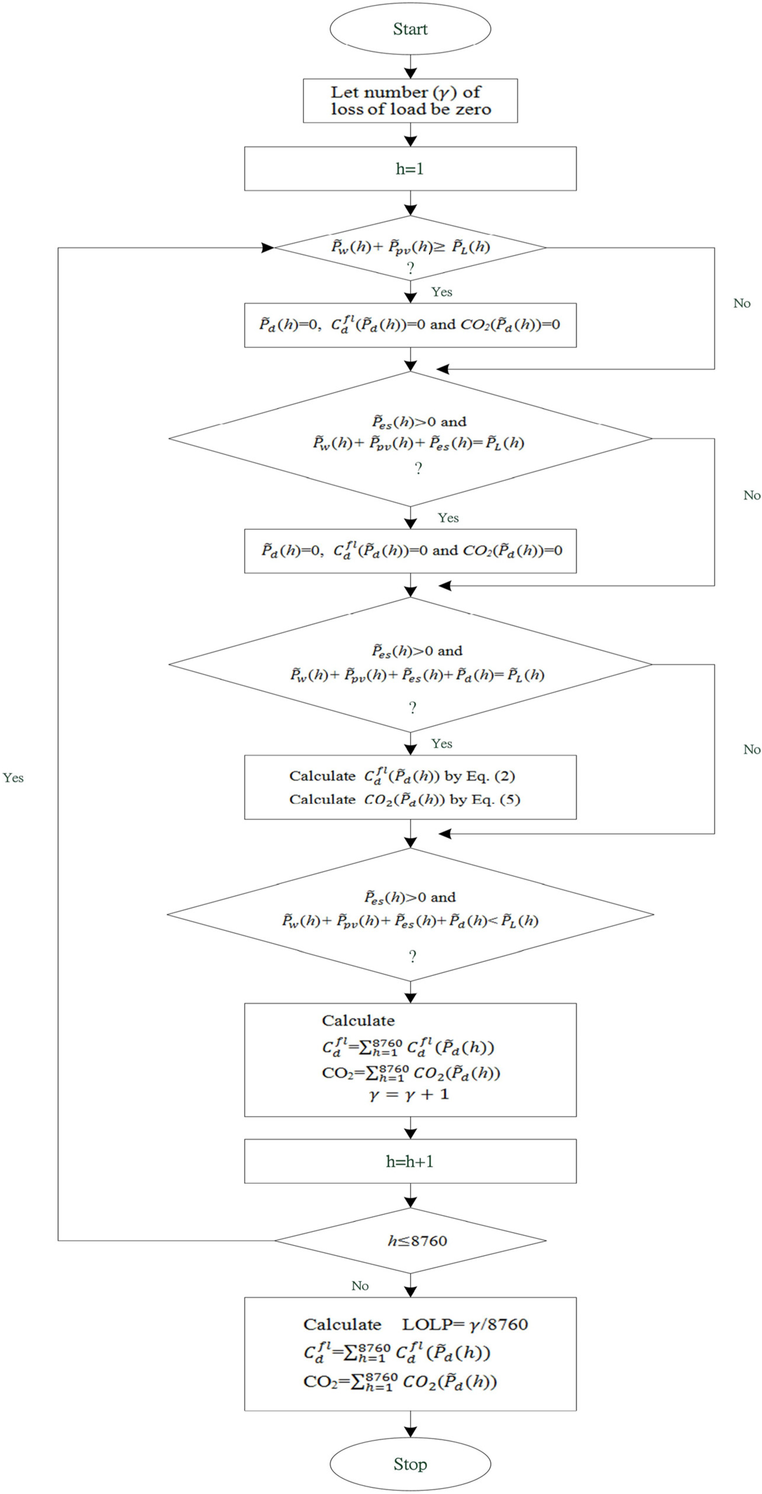
2.4. Estimation of LOLP and CO₂ Emission

The problem here is to determine the values of N_w, N_pv, N_es and N_d for given chronological data, including hourly probabilistic load, wind speed and irradiation/temperature over a period, for example 8760 h. Once these unknowns are evaluated by Genetic Algorithm (GA) herein, the LOLP in Equation (3) and the emission of CO₂ in Equation (4) can be determined using the chronological data. Let r be the index of the loss of load and ${\tilde{P}}_{es}(h)$ be the power generated by the ES at hour h. Figure 1 shows the flowchart for calculating the dependent variables, i.e., fuel cost, LOLP, and the emission of CO₂. Specifically, if ${\tilde{P}}_w(h)+{\tilde{P}}_{pv}(h)>{\tilde{P}}_L(h)$, then the ES is charging (${\tilde{P}}_{es}(h)$ <0); otherwise it is discharging (${\tilde{P}}_{es}(h)$ > 0).

Figure 1. Flowchart of calculating the fuel cost, LOLP and the emission of CO₂.

Figure 1. Flowchart of calculating the fuel cost, LOLP and the emission of CO₂.

The start and stop operations as well as the minimum operating powers of diesel generators should be considered in an operation problem, e.g., unit commitment and real power scheduling. However, in a planning problem, these factors were generally ignored [3,6,7,9,15,16]. In different load conditions, the efficiency of each diesel generator is different because the output power of each diesel generator is varied. In the planning stage, this factor can be ignored [3]; however, this issue incorporating with unit commitment should be considered in the operation stage.

3. Proposed Method

As described in Section 2, intermittent wind/PV and random load are modeled as probabilistic (stochastic) distributions in this paper. The steps for solving the problem are not straightforward because of the probabilistic/random variables with, for example, normal (Gaussian) or Weibull distributions, or discrete probabilities, and so on. Specifically, random variables are added and multiplied by convolution. Since convolution involves integration, searching an optimal solution requires considerable computational effort. To avoid convolution, this work utilizes cumulants and the Gram-Charlier series expansion to model the uncertainties of the renewable energies and loads [24,25].

3.1. Moment and Cumulant

The γ-th moment of a continuous random variable x is defined as follows:

$${\mathrm{\alpha }}_{\mathrm{\gamma }}={\displaystyle \underset{-\mathrm{\infty }}{\overset{\mathrm{\infty }}{\int }}{x}^{\mathrm{\gamma }}h(x)}dx$$

(8)

where $h(x)$ is the probability density function (PDF) of x. If a component $x_c$ of a discrete random variable χ has a corresponding probability $p_c$, then the γ-th moment of χ is defined as follows:

$${\mathrm{\alpha }}_{\mathrm{\gamma }}={\displaystyle {\sum }_{c=1}^{\mathrm{\infty }}{p}_c{x_c}^{\mathrm{\gamma }}}$$

(9)

The cumulants $k_{\mathrm{\gamma }}$ can be derived from the moments using recursion in closed forms as follows.

$$k_1={\mathrm{\alpha }}_1$$

(10)

$$k_2={\mathrm{\alpha }}_2-{\mathrm{\alpha }}_1^2$$

(11)

$$k_3={\mathrm{\alpha }}_3-3{\mathrm{\alpha }}_2{\mathrm{\alpha }}_1+2{\mathrm{\alpha }}_1^3$$

(12)

and so forth. The rest of the cumulants can be found elsewhere [25,26]. The terms $k_1$ and $k_2$ are defined as the expected value and the variance of the random variable, respectively. $k_{\mathrm{\gamma }}$ is generally neglected if $\mathrm{\gamma }\ge 9$.

3.2. Cumulant Effect

Let $X_k$, k = 1, 2, ..., K, be an independent random variable and $w_k$ be the k-th corresponding coefficients. Then the $\mathrm{\gamma }-th$ cumulant of ${\displaystyle {\sum }_{k=1}^K{w}_k\times X_k}$ equals the weighted sum of the K corresponding $\mathrm{\gamma }-th$ cumulants for $X_k$, k = 1, 2, ..., K. This equality is called the cumulant effect [27].

The cumulant effect is applied to compute the fuel cost in Equation (2) and the emission of CO₂ in Equation (5) without performing any convolution. Accordingly, the cumulants of ${\tilde{P}}_d$ are calculated first. The respective cumulants of fuel cost and the emission of CO₂ are then computed using the cumulant effect.

3.3. Expression of PDF Using Gram-Charlier Series Expansion

${\tilde{P}}_w(h)$, ${\tilde{P}}_{pv}(h)$ and ${\tilde{P}}_L(h)$ are given in terms of PDFs. Any dependent variable, such as ${\tilde{P}}_d(h)$, $C_d^{fl}$ (${\tilde{P}}_d(h)$), ${\tilde{P}}_{es}(h)$, and ${\tilde{P}}_{dif}(h)$, should therefore be expressed using PDFs. For example, the dependent variable ${\tilde{P}}_d(h)$ can be expressed by its PDF, as follows:

$$f(P_d(h))={\displaystyle \underset{P_d(h)}{\overset{\mathrm{\infty }}{\int }}N(P_d(h)})d{P}_d(h)+N({\overline{P}}_d(h)){\displaystyle \sum _{\mathrm{\gamma }=3}^8{a}_{\mathrm{\gamma }}}{H}_{\mathrm{\gamma }-1}(P_d(h))$$

(13)

Equation (13) is the Gram-Charlier series expansion. $H_{\mathrm{\gamma }-1}(P_d(h))$ is the Hermite polynomial [27]. The constant $a_{\mathrm{\gamma }}$ is the coefficient of the Hermite polynomial. $N(P_d(h))$ signifies the PDF for a normal distribution. ${\overline{P}}_d(h)$ is normalized $P_d(h)$.

3.4. Cumulative Probability

When the PDF of a dependent variable is gained using Equation (13), the representative of this dependent variable is the one for which the cumulative probability is ξ. This representative can be used to check the inequality constraints to evaluate the fuel cost in Equation (2) and to calculate SOC in Equation (7). From the viewpoint of statistics, we want to be as confident as possible when a population parameter is estimated. This is why confidence levels are generally very high. The most common confidence levels are 90%, 95%, and 99%. A 90% confidence interval approximately corresponds to the cumulative probability of 0.95 [28]. In this paper, ξ is set to be 0.95. Section 4 will investigate the effects of several possible values of ξ.

3.5. Genetic Algorithm

Searching the optimal N_w, N_pv, N_es and N_d in an autonomous power system is a probabilistic mixed integer programming (PMIP) problem. Specifically, the unknown N_w, N_pv, N_es, and N_d are integer variables and the unknown dependent variables at hour h are probabilistic. Traditional MIP cannot find optima [29] because variables and constraints are implicit and nonlinear, as shown in Equations (2)–(7).

In this paper, the GA is used to solve Equations (1)–(7). The variables N_w, N_pv, N_es, and N_d are regarded as a chromosome (gene string or individual) acting like independent variables, while others are the dependent ones. The lengths of binary bits required to specify N_w, N_pv, N_es, and N_d are 5, 8, 4, and 3, respectively. The chromosomes undergo crossover and mutation following their crossover and mutation rates, respectively [30].

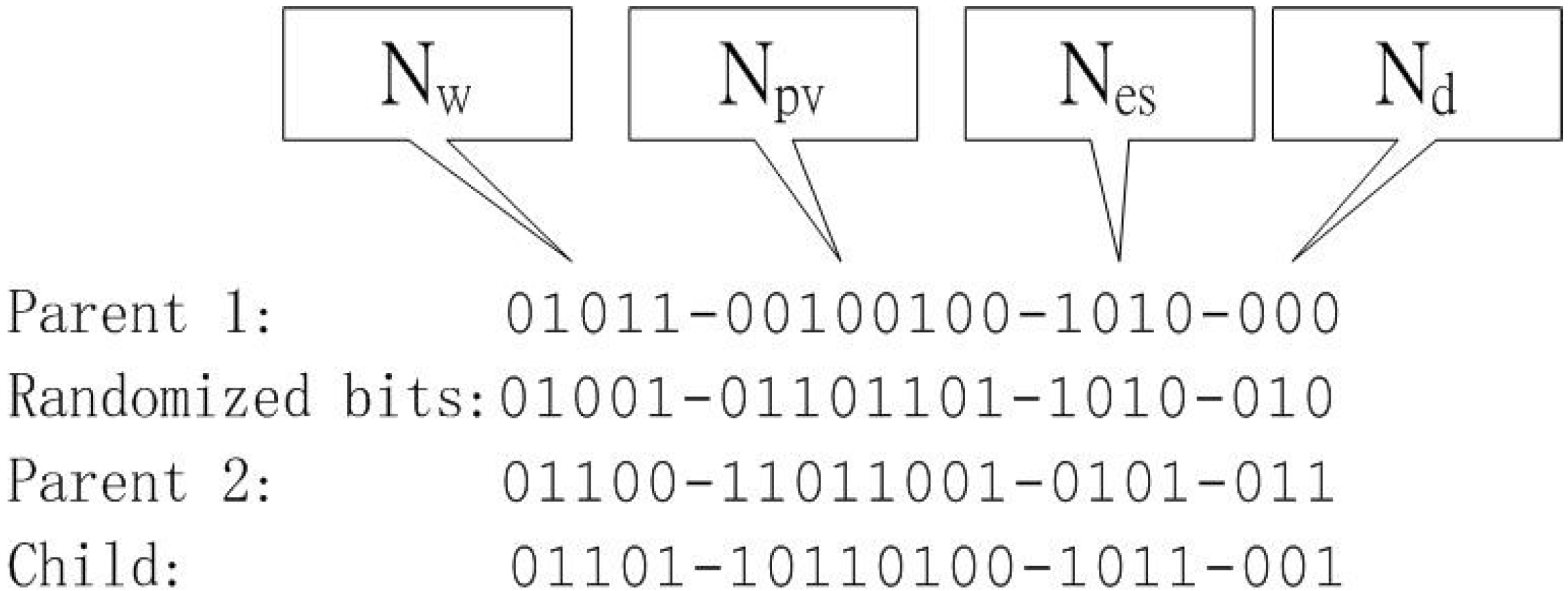
3.5.1. Crossover Operation

The crossover operation is performed by producing a random binary string first. Then select the genes from the 1^st parent if the corresponding randomized bits are “1”, and select the genes from the 2^nd parent if the corresponding randomized bits are “0”. Finally, a new child is gained by combining the selected genes. For example, given Parent_1 (=[a b c d e]) and Parent_2 (=[m n o p q]) are the parents and the randomized binary string is [1 0 1 0 1]. Then the child is [a n c p e]. Figure 2 illustrates another example for the crossover operation in the studied problem. Parents 1 and 2 have a total of 20 binary bits (5 + 8 + 4 + 3) to specify N_w, N_pv, N_es and N_d. Parent chromosomes are identified at random according to the crossover rate. The randomized binary bits are generated after any two parents are identified. Each bit of the child chromosome is gained by examining the bits in the corresponding positions of parent 1, the randomized binary string and parent 2.

Figure 2. Crossover operations applied to two parents.

Figure 2. Crossover operations applied to two parents.

3.5.2. Mutation Operation

This work utilized the Gaussian mutation operation. A random number produced from a Gaussian distribution is added to an identified binary bit of a chromosome according to the mutation rate. The mean and standard deviation of the Gaussian distribution are zero and ${\mathrm{\sigma }}_t$, respectively. The latter is determined adaptively as follows:

$${\mathrm{\sigma }}_{t+1}={\mathrm{\sigma }}_t\times (1-\frac{t}{\max \_\text{iteration}})$$

(14)

where t is the iteration index. The term “max_iteration” is the estimated maximum number of iterations. Once the mutation operation is done, the identified bit is rounded to the nearest 0 or 1.

3.5.3. Penalty Functions

This work utilizes the penalty functions that are augmented to Equation (1) to deal with the violated inequality constraints for the dependent variables (LOLP and emission of CO₂) in the roulette wheel selection operation [30]. For example, Equation (15) is the penalty function if Equation (3) is violated:

$$P{F}^{\frac{t}{N}}{(LOLP-LOL{P}^{\max })}^2$$

(15)

where PF is referred to as the “penalty factor” herein. Equation (15) specifies that the penalty weight (PF^t/N) has a greater impact on the violated amount after the N-th iteration (where N is a given number) than before the N-th iteration. The penalty factor has a positive sign. Consequently, a chromosome with a large fitness value owing to an augmented penalty term may have few opportunities to be selected in roulette wheel selection.

3.6. Steps of Algorithm

The steps for determining the optimal capacities of distributed generation resources and ES in a small autonomous power system considering uncertainty can be summarized as follows:

Step 1

Specify historical/hourly loads, wind speed, radiation/temperature using their corresponding PDFs. Read fuel coefficients and emission coefficients in Equations (2) and (5), respectively. Read operational limits, as well as reliability and limits on the emissions of greenhouse gases.

Step 2

Compute all cumulants of chronological ${\tilde{P}}_w(h)$, ${\tilde{P}}_{pv}(h)$ and ${\tilde{P}}_L(h)$, h = 1, 2, …, 8760.

Step 3

Specify the population size (p = 1, 2, …, P), crossover rate and mutation rate in the GA. Define Equation (1) as the fitness in the GA. Encode all chromosomes.

Step 4

Conduct the crossover and mutation operations according to Figure 2 and Equation (14), respectively, on all of the chromosomes in the mating pool.

Step 5

Decode all of the chromosomes and compute their corresponding fitness functions. Let p = 1.

Step 6

Compute all cumulants of hourly ${\tilde{P}}_d(h)$, ${\tilde{P}}_{es}(h)$ and ${\tilde{P}}_{dif}(h)$.

Step 7

Execute the steps shown in Figure 1 using the cumulant effect in Section 3.2 and the Gram-Charlier series expansion in Section 3.3 to gain the hourly fuel cost and emission of CO₂. Compute the LOLP.

Step 8

If emission of CO₂ or LOLP violate Equation (3) or Equation (4), respectively, then add the corresponding penalty term to the fitness. Let p = p + 1.

Step 9

If p = P, then conduct the roulette wheel selection based on all fitness values plus their corresponding penalty terms to identify better chromosomes for the next generation (iteration); otherwise, go to Step 6.

Step 10

If the termination criterion in GA is fulfilled, then stop; otherwise, go to Step 4.

4. Simulation Results

4.1. Test Data

A small autonomous power system with 150 kW peak load was studied in this paper. The 8760 h load profile in the IEEE Reliability Test System (RTS) was used [3,13,22]. Assume that the hourly load follows a Gaussian distribution. Table 1 shows the 1^st–8^th cumulants of four load levels (others are not shown). The historical weather data (m/s and W/m²) for Mt. Jade (23°28′12″ N, 120°57′16″ E) in Taiwan were modeled by Weibull distribution (f(x) = (κ/c)(x/c) ^κ−1exp(−(x/c)^κ) where x denotes the wind speed or radiation, and κ and c represent the scale and shape parameters, respectively [31]. Table 2 and Table 3 show the cumulants of power generated by the PV and wind-turbines that correspond to some parameters κ and c, respectively. The first columns in Table 1, Table 2 and Table 3 are the mean values of power levels. In Table 1, the mean value of the Gaussian distribution is the same as k₁, while in Table 2 and Table 3, the mean value of the Weibull distribution differs from k₁.

Table 2. Cumulants of PV power levels with different values of κ and c.

	Cumulants	k1	k2	k3	k4	k5	k6	k7	k8	κ	c
Mean Value (kW)
0		0	0	0	0	0	0	0	0	0	0
1		1	0.29	0.11	0.03	−0.01	−0.03	−0.01	0.02	1.92	1.13
2		1.95	1.09	0.52	−0.38	−1.75	−1.47	9.42	38.81	1.92	2.25
3		2.27	1.98	−0.10	−3.80	1.70	34.97	−40.62	−721.60	1.92	3.38
4		2.02	2.78	0.47	−10.69	−5.73	187.24	202.24	−7127.65	1.92	4.51
5		1.65	3.08	2.43	−12.92	−46.77	205.74	1972.06	−5151.88	1.92	5.64

Table 2. Cumulants of PV power levels with different values of κ and c.

	Cumulants	k1	k2	k3	k4	k5	k6	k7	k8	κ	c
Mean Value (kW)
0		0	0	0	0	0	0	0	0	0	0
1		1	0.29	0.11	0.03	−0.01	−0.03	−0.01	0.02	1.92	1.13
2		1.95	1.09	0.52	−0.38	−1.75	−1.47	9.42	38.81	1.92	2.25
3		2.27	1.98	−0.10	−3.80	1.70	34.97	−40.62	−721.60	1.92	3.38
4		2.02	2.78	0.47	−10.69	−5.73	187.24	202.24	−7127.65	1.92	4.51
5		1.65	3.08	2.43	−12.92	−46.77	205.74	1972.06	−5151.88	1.92	5.64

Table 3. Cumulants of wind power levels with different values of κ and c.

	Cumulants	k1	k2	k3	k4	k5	k6	k7	k8	κ	c
Mean Value (kW)
1		0.00	0.00	0.00	0.00	0.00	0.00	0.00	0.00	2.09	1.13
2		0.00	0.00	0.00	0.00	0.00	0.00	0.00	0.00	2.09	2.26
3		0.00	0.00	0.00	0.00	0.00	0.00	0.00	0.00	2.09	3.39
4		0.71	0.13	0.03	0.00	0.00	0.00	0.00	0.00	2.09	4.52
5		1.96	0.97	0.55	0.14	−0.35	−0.62	0.34	3.80	2.09	5.65
6		3.55	3.19	3.27	1.47	−6.93	−22.30	21.98	447.33	2.09	6.77
7		5.69	8.19	13.46	9.69	−73.20	−377.73	588.18	19279.99	2.09	7.90
8		8.50	18.26	44.07	29.77	−881.21	−9169.61	−42543.18	362872.76	2.09	9.03
9		11.83	33.43	72.77	−583.69	−9792.04	654.93	2348606.58	27695330.20	2.09	10.16
10		14.66	43.78	5.12	−1972.94	−4199.98	436344.29	2452126.18	−214451973.79	2.09	11.29
11		16.44	46.68	−86.07	−2373.78	18354.16	562769.22	−9865268.34	−278693443.05	2.09	12.42
12		17.43	46.71	−144.73	−2181.18	33451.46	390646.31	−17658764.09	−75117959.02	2.09	13.55
13		17.99	46.18	−177.17	−1921.18	40831.90	209668.99	−20357252.19	109887544.59	2.09	14.68
14		18.30	45.69	−195.17	−1723.07	44353.03	82809.21	−21009161.82	228049326.78	2.09	15.81
15		18.49	45.33	−205.53	−1589.07	46125.72	1104.68	−21029440.75	299107504.35	2.09	16.94
16		18.61	45.09	−211.75	−1500.91	47081.72	−51002.13	−20896556.67	342264715.14	2.09	18.06
17		18.68	44.92	−215.62	−1442.93	47630.29	−4579.68	−20753607.19	369147090.12	2.09	19.19
18		18.73	44.82	−217.92	−1407.30	47938.09	−104946.27	−20645504.59	385087512.06	2.09	20.32
19		18.72	44.82	−217.85	−1408.36	47929.23	−104342.60	−20648939.01	384619064.86	2.09	21.45
20		18.61	45.08	−211.82	−1499.90	47091.81	−51591.81	−20894429.02	342743182.03	2.09	22.58
21		18.28	45.73	−193.77	−1739.94	44098.84	93321.82	−20985139.89	218614684.56	2.09	23.71
22		17.64	46.56	−157.07	−2096.11	36383.05	329057.29	−18877917.19	−9884837.14	2.09	24.84
23		16.65	46.79	−98.23	−2361.63	21566.73	543424.55	−11651899.31	−252122928.12	2.09	25.97
24		15.30	45.21	−24.47	−2206.51	2494.17	529969.56	−939087.82	−283408170.14	2.09	27.10
25		13.68	40.82	41.12	-1497.48	-10327.79	252315.74	4641727.93	−86303510.97	2.09	28.23

Table 3. Cumulants of wind power levels with different values of κ and c.

	Cumulants	k1	k2	k3	k4	k5	k6	k7	k8	κ	c
Mean Value (kW)
1		0.00	0.00	0.00	0.00	0.00	0.00	0.00	0.00	2.09	1.13
2		0.00	0.00	0.00	0.00	0.00	0.00	0.00	0.00	2.09	2.26
3		0.00	0.00	0.00	0.00	0.00	0.00	0.00	0.00	2.09	3.39
4		0.71	0.13	0.03	0.00	0.00	0.00	0.00	0.00	2.09	4.52
5		1.96	0.97	0.55	0.14	−0.35	−0.62	0.34	3.80	2.09	5.65
6		3.55	3.19	3.27	1.47	−6.93	−22.30	21.98	447.33	2.09	6.77
7		5.69	8.19	13.46	9.69	−73.20	−377.73	588.18	19279.99	2.09	7.90
8		8.50	18.26	44.07	29.77	−881.21	−9169.61	−42543.18	362872.76	2.09	9.03
9		11.83	33.43	72.77	−583.69	−9792.04	654.93	2348606.58	27695330.20	2.09	10.16
10		14.66	43.78	5.12	−1972.94	−4199.98	436344.29	2452126.18	−214451973.79	2.09	11.29
11		16.44	46.68	−86.07	−2373.78	18354.16	562769.22	−9865268.34	−278693443.05	2.09	12.42
12		17.43	46.71	−144.73	−2181.18	33451.46	390646.31	−17658764.09	−75117959.02	2.09	13.55
13		17.99	46.18	−177.17	−1921.18	40831.90	209668.99	−20357252.19	109887544.59	2.09	14.68
14		18.30	45.69	−195.17	−1723.07	44353.03	82809.21	−21009161.82	228049326.78	2.09	15.81
15		18.49	45.33	−205.53	−1589.07	46125.72	1104.68	−21029440.75	299107504.35	2.09	16.94
16		18.61	45.09	−211.75	−1500.91	47081.72	−51002.13	−20896556.67	342264715.14	2.09	18.06
17		18.68	44.92	−215.62	−1442.93	47630.29	−4579.68	−20753607.19	369147090.12	2.09	19.19
18		18.73	44.82	−217.92	−1407.30	47938.09	−104946.27	−20645504.59	385087512.06	2.09	20.32
19		18.72	44.82	−217.85	−1408.36	47929.23	−104342.60	−20648939.01	384619064.86	2.09	21.45
20		18.61	45.08	−211.82	−1499.90	47091.81	−51591.81	−20894429.02	342743182.03	2.09	22.58
21		18.28	45.73	−193.77	−1739.94	44098.84	93321.82	−20985139.89	218614684.56	2.09	23.71
22		17.64	46.56	−157.07	−2096.11	36383.05	329057.29	−18877917.19	−9884837.14	2.09	24.84
23		16.65	46.79	−98.23	−2361.63	21566.73	543424.55	−11651899.31	−252122928.12	2.09	25.97
24		15.30	45.21	−24.47	−2206.51	2494.17	529969.56	−939087.82	−283408170.14	2.09	27.10
25		13.68	40.82	41.12	-1497.48	-10327.79	252315.74	4641727.93	−86303510.97	2.09	28.23

The studied unit capacities of the diesel generator, WTG, PV and ES are 25, 25, 5, and 1 kW, respectively. Their corresponding $N_d^{\max }$, $N_w^{\max },$$N_{pv}^{\max },$ and $N_{es}^{\max }$ are 7, 63, 127, and 31, respectively. Table 4 presents the costs of the units, installation and maintenance. The prices of WTG and PV are similar to those in [6,14]. More specifically, the cost of ES in Table 4 includes that of the inverter; the ratings of one unit of the ES are 104 Ah and 12 V. The ES can run the standalone mode using either master control (voltage/frequency) or slave control (real/reactive power control). The fuel coefficients, a ($/h), b ($/kWh) and c ($/kW²h), for the diesel generator that are used in Equation (2) are 1.07, 0.0657 and 0.00006, respectively; the emission coefficients, d (kg/h), e (kg/kWh) and f (kg/kW²h), in Equation (5) are 28.144, 1.728 and 0.0017, respectively.

Table 4. Costs for diesel, WTG, PV, and ES units.

DG/ES	Unit Cost	Installation Cost ($/kW)	Maintenance Cost
Diesel	300 $/kW	600	0.02 $/kWh
WTG	1500 $/kW	600	0.06 $/kW
PV	8000 $/kW	-	-
ES	300 $/kWh	-	-

Table 4. Costs for diesel, WTG, PV, and ES units.

DG/ES	Unit Cost	Installation Cost ($/kW)	Maintenance Cost
Diesel	300 $/kW	600	0.02 $/kWh
WTG	1500 $/kW	600	0.06 $/kW
PV	8000 $/kW	-	-
ES	300 $/kWh	-	-

The population size, crossover rate, and mutation rate in the GA are 20, 0.8 and 0.02, respectively. A chromosome consists of 20 binary bits (see Figure 2).

A MATLAB code was developed to implement the algorithm on a PC with an Intel(R) Core(TM) i5-2500k CPU@3.3 GHZ, 8 GB RAM.

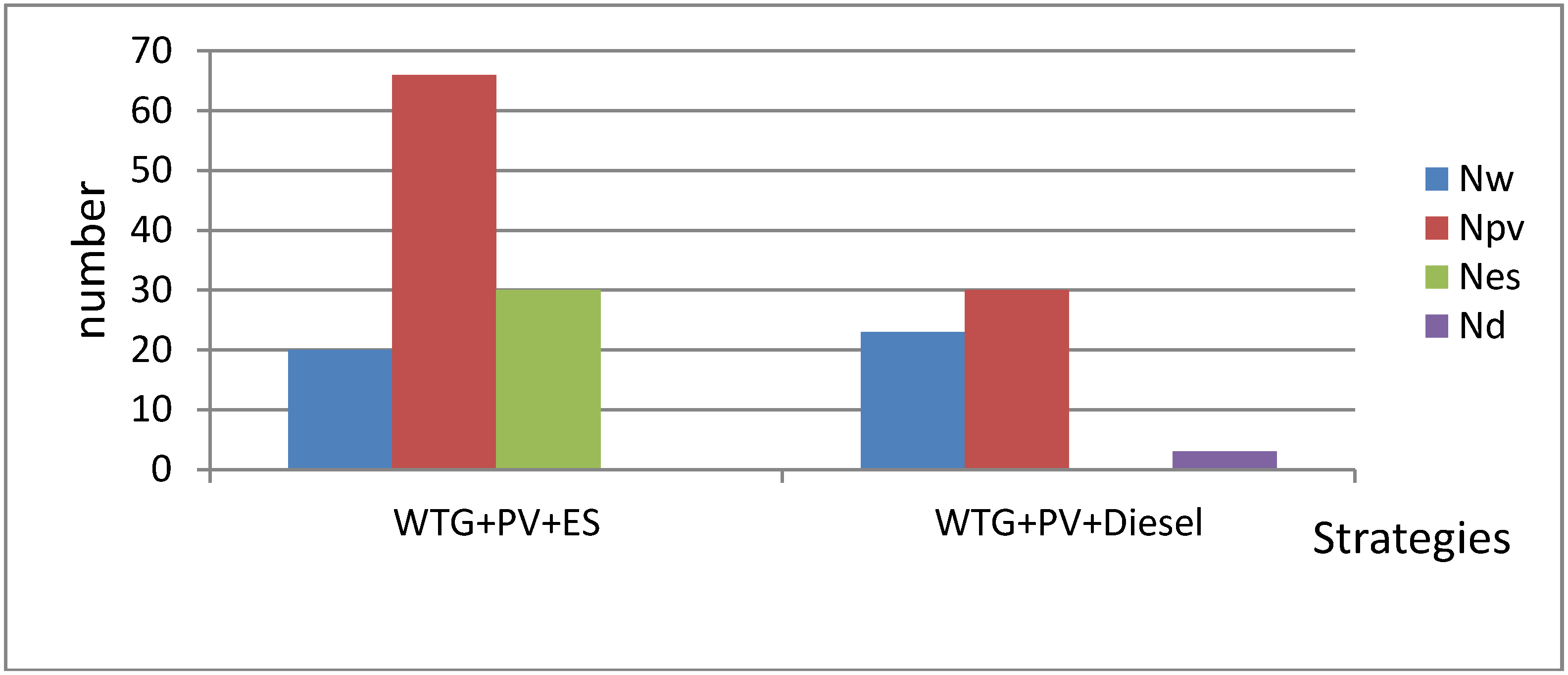
4.2. Results without Considering Diesel Generation or Energy Storage

Due to uncertainty in the power generated by WTG and PV, diesel generators or energy storage are needed to maintain reliability. Assume LOLP^max = 0.03 and CO₂^max = 50,000 kg/year. The representative of a dependent variable is the value whose cumulative probability ξ is 95%. Two strategies were explored herein: (i) WTG + PV + ES; (ii) WTG + PV + Diesel. Figure 3 illustrates the numbers of WTG, PV, ES and diesel generators. As shown in Table 5, Strategy (i) with ES costs more than Strategy (ii) with diesel generators. However, diesel generation emits a large amount of CO₂ (49,821 kg/y). Strategy (i) with ES requires much more CPU time because of required SOC evaluation in Equation (7).

Figure 3. Numbers of WTG, PV, ES, and diesel generators considering two different strategies.

Figure 3. Numbers of WTG, PV, ES, and diesel generators considering two different strategies.

Table 5. Results obtained by two strategies.

Strategies	Total Cost ($)	LOLP	CO2 (kg/y)	CPU (s)
WTG + PV + ES	3,699,000	0.030	-	203.50
WTG + PV + Diesel	2,476,926	0.028	49,821	28.71

Table 5. Results obtained by two strategies.

Strategies	Total Cost ($)	LOLP	CO2 (kg/y)	CPU (s)
WTG + PV + ES	3,699,000	0.030	-	203.50
WTG + PV + Diesel	2,476,926	0.028	49,821	28.71

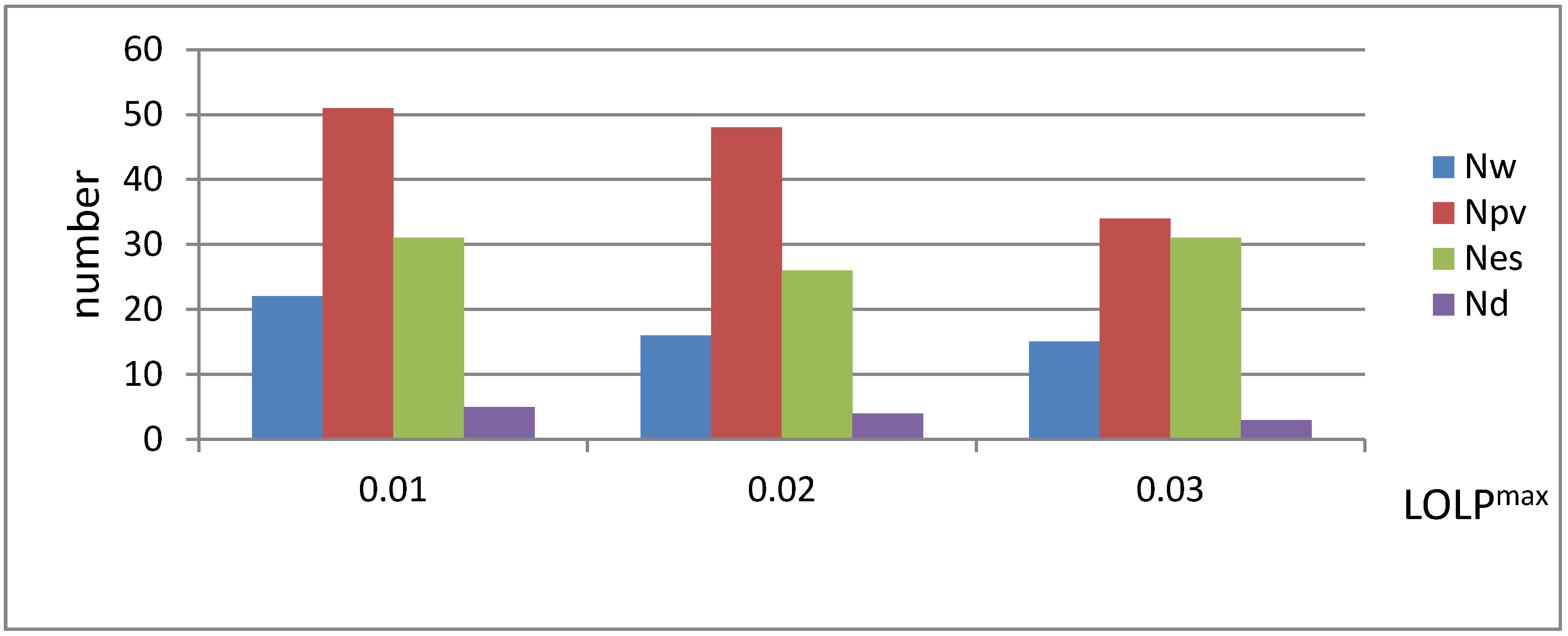
4.3. Impacts of Different LOLP Constraints

This section investigates the impacts of different values of LOLP^max on cost, emissions of CO₂ and CPU time. Assume that CO₂^max is 50,000 kg/year. Figure 4 illustrates the numbers of WTG, PV, ES and diesel generators. Table 6 indicates that a high reliability (small LOLP^max) results in a high investment cost. Also, a small LOLP^max requires a short CPU time because the searched solution space is small. The wind speed is high at night in winter, while solar irradiation is strong during the day in summer. The loss of load happens at different times in the summer and the winter. As LOLP^max declines (from 0.03 to 0.01), more diesel generators (from three to five) are needed. It can be found that all CO₂ emissions meet the constraint limits.

Figure 4. Numbers of WTG, PV, ES, and diesel generators considering different LOLP^max.

Figure 4. Numbers of WTG, PV, ES, and diesel generators considering different LOLP^max.

Table 6. Result comparison between different LOLP constraints.

LOLPmax	Total Cost ($)	LOLP	CO2 (kg/y)	CPU (s)
0.01	3,318,728	0.004	49,938	57.8
0.02	2,859,729	0.015	49,945	73.2
0.03	2,226,227	0.024	49,882	93.9

Table 6. Result comparison between different LOLP constraints.

LOLPmax	Total Cost ($)	LOLP	CO2 (kg/y)	CPU (s)
0.01	3,318,728	0.004	49,938	57.8
0.02	2,859,729	0.015	49,945	73.2
0.03	2,226,227	0.024	49,882	93.9

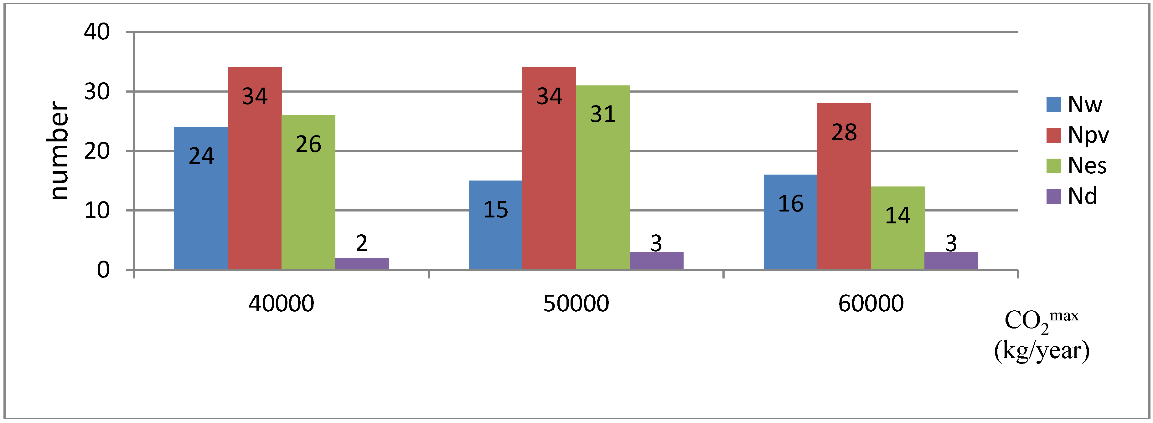
4.4. Impacts of Different CO₂ Constraints

This subsection explores the effects of different values of CO₂^max on cost, LOLP and CPU time. LOLP^max is fixed at 0.03. Figure 5 illustrates the numbers of WTG, PV, ES and diesel generators. Table 7 implies that a small CO₂^max results in a high cost because more renewables and fewer diesel generators are needed. When the CO₂ limit becomes stricter (lower emissions), less CPU time is required because the solution space shrinks.

Figure 5. Numbers of WTG, PV, ES, and diesel generators considering different CO₂^max.

Figure 5. Numbers of WTG, PV, ES, and diesel generators considering different CO₂^max.

Table 7. Result comparison between different CO₂ constraints.

CO2max (kg/year)	Total Cost ($)	LOLP	CO2 (kg/y)	CPU (s)
4 × 104	2,674,314	0.030	39,161	85.0
5 × 104	2,226,227	0.024	49,882	93.9
6 × 104	2,033,995	0.029	59,379	137.2

Table 7. Result comparison between different CO₂ constraints.

CO2max (kg/year)	Total Cost ($)	LOLP	CO2 (kg/y)	CPU (s)
4 × 104	2,674,314	0.030	39,161	85.0
5 × 104	2,226,227	0.024	49,882	93.9
6 × 104	2,033,995	0.029	59,379	137.2

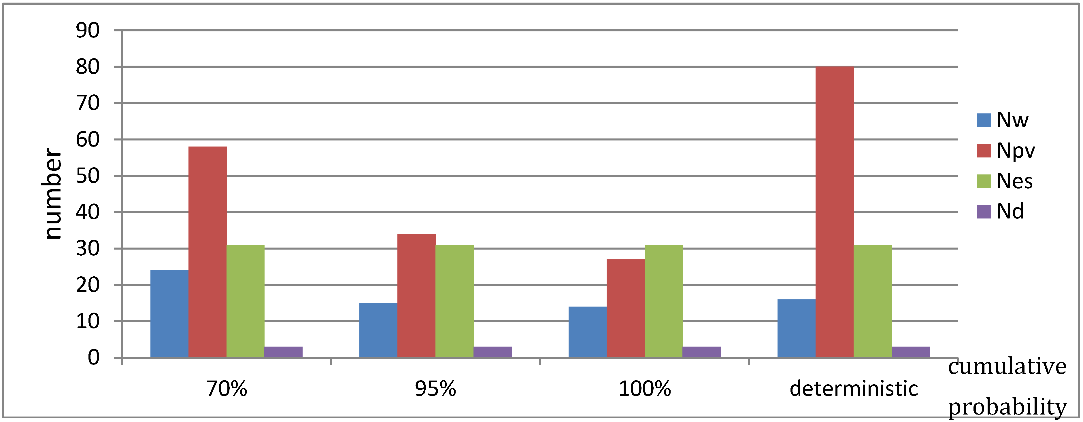
4.5. Effect of Cumulative Probability

This section investigates the effects of the cumulative probability ξ (70%, 95% and 100%) on the solutions. For comparison, the deterministic solution that considers only the expected values (that is, k₁) of random variables is also given. LOLP^max and CO₂^max are 0.03 and 50,000 kg/y here, respectively. Figure 6 illustrates the numbers of WTG, PV, ES and diesel generators. Table 8 reveals that the cost is the lowest when ξ = 100% because ξ = 100% maximizes ${\tilde{P}}_w(h)$ and ${\tilde{P}}_{pv}(h)$ (Weibull distribution), which have a larger effect on ${\tilde{P}}_w(h)$ and ${\tilde{P}}_{pv}(h)$ than ${\tilde{P}}_L(h)$ (which follows a Gaussian distribution). The deterministic solution yields the highest cost because the expected value of the Weibull distribution is biased toward the left but that of the Gaussian distribution is centered. The effect of hourly load on total cost is, therefore, larger than that of the hourly power generation from renewable sources.

Figure 6. Numbers of WTG, PV, ES, and diesel generators considering deterministic method and different cumulative probabilities.

Figure 6. Numbers of WTG, PV, ES, and diesel generators considering deterministic method and different cumulative probabilities.

Table 8. Result comparison between different cumulative probabilities.

Cumulative Probabilities	Total Cost ($)	LOLP	CO2 (kg/y)	CPU (s)
ξ = 70%	3,658,728	0.022	49,894	117.0
ξ = 95%	2,226,227	0.024	49,882	93.9
ξ = 100%	1,893,731	0.027	49,969	69.0
deterministic	4,118,731	0.022	49,989	100.3

Table 8. Result comparison between different cumulative probabilities.

Cumulative Probabilities	Total Cost ($)	LOLP	CO2 (kg/y)	CPU (s)
ξ = 70%	3,658,728	0.022	49,894	117.0
ξ = 95%	2,226,227	0.024	49,882	93.9
ξ = 100%	1,893,731	0.027	49,969	69.0
deterministic	4,118,731	0.022	49,989	100.3

4.6. Impacts of Different Initial SOCs

This subsection examines the impacts of different initial SOCs (50%, 70% and 85%) on the final optimal solutions. It is not surprising that final results about the numbers of WTG, PV, ES, and diesel generators are the same for these three different initial conditions. The reason is that a rate of 1 C is considered as described in Section 2.3. A rate of 1 C means one hour is needed to fully charge the battery from an empty state. Thus, if initial SOC = 50%, then it needs only 21 min, which is smaller than one hour (time interval in this paper), to charge to its maximum limit (85% herein). Thus, if the WTG has surplus energy initially, then the SOC of ES will reach the maximum limit in the initial hours. Table 9 shows the result comparison between different initial SOCs.

Table 9. Result comparison between different initial state-of-charges.

SOC	Total Cost ($)	LOLP	CO2 (kg/y)	CPU (s)
SOC = 50%	2,227,112	0.023	49,997	95.0
SOC = 70%	2,226,603	0.024	49,955	94.4
SOC = 85%	2,226,227	0.024	49,882	93.9

Table 9. Result comparison between different initial state-of-charges.

SOC	Total Cost ($)	LOLP	CO2 (kg/y)	CPU (s)
SOC = 50%	2,227,112	0.023	49,997	95.0
SOC = 70%	2,226,603	0.024	49,955	94.4
SOC = 85%	2,226,227	0.024	49,882	93.9

4.7. Discussions

The above results support the following comments:

(1)

Energy storage effectively provides an emission-free generation resource that supports reliability but is much more costly than diesel generators.

(2)

Strict LOLP and CO₂ emission limits require large investments to ensure the supply of high quality power and low emissions in a small autonomous power system.

(3)

The CPU times required to perform simulations are approximately 1–3 min if the energy storage system is considered. If no energy storage system is considered, then a simulation takes only around 30 s. The CPU time that is required by the proposed method is independent of the number of buses/lines.

(4)

The required CPU time may increase if more data from more years (two or three) are used to increase the accuracy of the evaluation of reliability, meaning that a longer planning horizon is considered. In this case, the expected lifetimes of all generation resources and the energy storage system should be evaluated.

(5)

The deterministic study yields a pessimistic solution with the largest cost among all approaches. A large cumulative probability ξ yields an optimistic solution. The cost ($2,226,227), obtained with ξ = 95%, which is widely acceptable, is less than a half of that ($4,118,731) obtained by the deterministic study.

5. Conclusions

This paper presents a new method, based on the genetic algorithms, for determining the optimal capacities of hybrid wind/PV/diesel generation units and energy storage in a small autonomous power system. Historical 8760 h wind speed and solar irradiation data were used along with a forecast load profile, all of which were modeled by random variables to determine the optimal capacities of different distributed generation and energy storage. The PDF based on the Gram-Charlier series expansion is used to express uncertainty of renewables and loads.

The advantages of the method proposed herein can be summarized as follows. (1) Both optimization and reliability are implemented together while the greenhouse gas emission constraint is also considered by the inequality constraint. Traditional methods considered either optimization or reliabilityonly; (2) The meteorological data and loads were modeled as random variables using the Gram-Charlier series expansion, to avoid complex calculation.

The simulation results reveal that the reliability and greenhouse gas emission limits strongly affect the cost of the distributed generation resources and energy storage. The simulation results also indicate that the proposed uncertainty-based method yields a more optimistic result with a smaller cost than the deterministic method.

Future studies will consider the annualized costs of the WTG, PV, ES, and diesel generators using suitable life expectancy estimation models. The net present cost and capital recovery factor will be considered.

References

- Kyoto Protocol to the United Nations Framework Convention on Climate Change; United Nations: Bonn, Germany, 1997.
- The Copenhagen Accord. In Proceedings of the United Nations Climate Change Conference, Copenhagen, Denmark, 7–18 December 2009.
- Billinton, R.; Karki, R. Apacity expansion of small isolated power systems using PV and wind energy. IEEE Trans. Power Syst. 2001, 16, 892–897. [Google Scholar] [CrossRef]
- Ai, B.; Yang, H.; Shen, H.; Liao, X. Computer-aided design of PV/wind hybrid system. Renew. Energy 2003, 28, 1491–1512. [Google Scholar] [CrossRef]
- Nelson, D.B.; Nehrir, M.H.; Wang, C. Unit sizing and cost analysis of stand-alone hybrid wind/PV/fuel cell power generation systems. Renew. Energy 2006, 31, 1641–1656. [Google Scholar] [CrossRef]
- Diaf, S.; Diaf, D.; Belhamel, M.; Haddadi, M. A methodology for optimal sizing of autonomous hybrid PV/wind system. Energy Policy 2007, 35, 5708–5718. [Google Scholar] [CrossRef]
- Katsigiannis, Y.A.; Georgilakis, P.S.; Karapidakis, E.S. Hybrid simulated annealing—Tabu search method for optimal sizing of autonomous power systems with renewable. IEEE Trans. Sustain. Energy 2012, 3, 330–338. [Google Scholar] [CrossRef]
- Vrettos, E.I.; Papathanassiou, S.A. Operating policy and optimal sizing of a high penetration RES-BESS system for small isolated grids. IEEE Trans. Energy Convers. 2011, 26, 744–756. [Google Scholar] [CrossRef]
- Belfkira, R.; Zhang, L.; Barakat, G. Optimal sizing study of hybrid wind/PV/diesel power generation unit. Sol. Energy 2011, 85, 100–110. [Google Scholar] [CrossRef]
- Cabral, C.V.T.; Filho, D.O.; Diniz, A.S.A.C.; Martins, J.H. A stochastic method for stand-alone photovoltaic system sizing. Sol. Energy 2010, 84, 1628–1636. [Google Scholar] [CrossRef]
- Lujano-Rojas, J.M.; Dufo-López, R.; Bernal-Agustín, J.L. Probabilistic modelling and analysis of stand-alone hybrid power systems. Energy 2013, 63, 19–27. [Google Scholar] [CrossRef]
- Lujano-Rojas, J.M.; Dufo-Lopez, R.; Bernal-Agustin, J.L. Optimal sizing of small wind/battery systems considering the DC bus voltage stability effect on energy capture, wind speed variability, and load uncertainty. Appl. Energy 2012, 93, 404–412. [Google Scholar] [CrossRef]
- Kaviani, A.K.; Riahy, G.H.; Kouhsari, S.H.M. Optimal design of a reliable hydrogen-based stand-alone wind/PV generating system, considering component outages. Renew. Energy 2009, 34, 2380–2390. [Google Scholar] [CrossRef]
- Chen, S.G. Bayesian approach for optimal PV system sizing under climate change. Omega 2013, 41, 176–185. [Google Scholar] [CrossRef]
- Borhanazad, H.; Mekhilef, S.; Ganapathy, V.G.; Modiri-Delshad, M. Optimization of micro-grid system using MOPSO. Renew. Energy 2014, 71, 295–306. [Google Scholar] [CrossRef]
- Sharafi, M.; ELMekkawy, T.Y. Multi-objective optimal design of hybrid renewable energy systems using PSO-simulation based approach. Renew. Energy 2014, 68, 67–79. [Google Scholar] [CrossRef]
- Diaf, S.; Notton, G.; Belhamel, M.; Haddadi, M. Design and techno-economical optimization for hybrid PV/wind system under various meteorological conditions. Appl. Energy 2008, 85, 968–987. [Google Scholar] [CrossRef]
- Kaldellis, J.K. Optimum autonomous wind-power system sizing for remote consumers using long-term wind speed data. Appl. Energy 2002, 71, 215–233. [Google Scholar] [CrossRef]
- Luna-Rubio, R.; Trejo-Perea, M.; Vargas-Va’zquez, D.; Rı’os-Moreno, G.J. Optimal sizing of renewable hybrids energy systems: A review of methodologies. Sol. Energy 2012, 86, 1077–1088. [Google Scholar] [CrossRef]
- Atwa, Y.M.; el-Saadany, E.F. Probabilistic approach for optimal allocation of wind based distributed generation in distribution systems. IET Renew. Power Gener. 2011, 5, 79–88. [Google Scholar] [CrossRef]
- Soroudi, A.; Caire, R.; Hadjsaid, N.; Ehsan, M. Probabilistic dynamic multi-objective model for renewable and non-renewable distributed generation planning. IET Gener. Transm. Distrib. 2011, 5, 1173–1182. [Google Scholar] [CrossRef]
- Reliability Test System Task Force of the Application of Probability Methods Subcommittee. IEEE reliability test system. IEEE Trans. Power Syst. 1999, 14, 1010–1020. [Google Scholar]
- Alsema, E.A. Energy pay-back time and CO2 emissions of PV systems. Prog. Photovolt. Res. Appl. 2000, 8, 17–25. [Google Scholar] [CrossRef]
- Wang, C.S.; Liu, M.X.; Guo, L. Cooperative operation and optimal design for islanded microgrid. In Proceedings of the 2012 IEEE PES Innovative Smart Grid Technologies, Washington, DC, USA, 16–20 January 2012.
- Zhang, P.; Lee, S.T. Probabilistic load flow computation using the method of combined cumulants and Gram-Charlier expansion. IEEE Trans. Power Syst. 2004, 19, 676–681. [Google Scholar] [CrossRef]
- Hong, Y.Y.; Luo, Y.F. Optimal VAR control considering wind farms using probabilistic load flow and Gray-based genetic algorithms. IEEE Trans. Power Deliv. 2009, 24, 1441–1449. [Google Scholar] [CrossRef]
- Stuart, A.; Stuartx, J.K. Kendall’s Advanced Theory of Statistic, Distribution Theory, 6th ed.; Edward Arnold: London, UK, 1994; Volume 1. [Google Scholar]
- Review of Basic Statistical Concepts. Available online: http://sites.stat.psu.edu/~lsimon/stat501wc/sp05/00review/ (accessed on 20 March 2015).
- Taha, H.A. Integer Programming: Theory, Application and Computation; Academic Press: New York, NY, USA, 1975. [Google Scholar]
- Gen, M.; Cheng, R. Genetic Algorithms and Engineering Design; Wiley: New York, NY, USA, 1997. [Google Scholar]
- Keyhani, A. Design of Smart Power Grid Renewable Energy Systems; Wiley-IEEE Press: Hoboken, NJ, USA, 2011. [Google Scholar]
© 2015 by the authors; licensee MDPI, Basel, Switzerland. This article is an open access article distributed under the terms and conditions of the Creative Commons Attribution license (http://creativecommons.org/licenses/by/4.0/).
Share and Cite
Hong, Y.-Y.; Lai, Y.-M.; Chang, Y.-R.; Lee, Y.-D.; Liu, P.-W. Optimizing Capacities of Distributed Generation and Energy Storage in a Small Autonomous Power System Considering Uncertainty in Renewables. Energies 2015, 8, 2473-2492. https://doi.org/10.3390/en8042473
Hong Y-Y, Lai Y-M, Chang Y-R, Lee Y-D, Liu P-W. Optimizing Capacities of Distributed Generation and Energy Storage in a Small Autonomous Power System Considering Uncertainty in Renewables. Energies. 2015; 8(4):2473-2492. https://doi.org/10.3390/en8042473
Chicago/Turabian StyleHong, Ying-Yi, Yuan-Ming Lai, Yung-Ruei Chang, Yih-Der Lee, and Pang-Wei Liu. 2015. "Optimizing Capacities of Distributed Generation and Energy Storage in a Small Autonomous Power System Considering Uncertainty in Renewables" Energies 8, no. 4: 2473-2492. https://doi.org/10.3390/en8042473
APA StyleHong, Y.-Y., Lai, Y.-M., Chang, Y.-R., Lee, Y.-D., & Liu, P.-W. (2015). Optimizing Capacities of Distributed Generation and Energy Storage in a Small Autonomous Power System Considering Uncertainty in Renewables. Energies, 8(4), 2473-2492. https://doi.org/10.3390/en8042473