Energy’s Shadow Price and Energy Efficiency in China: A Non-Parametric Input Distance Function Analysis

Abstract

This paper extends prior research on energy inefficiency in China by utilizing a unique shadow price framework allocation in 30 Chinese provinces. We estimate the shadow price for energy input using the framework of production, and use the ratio of the shadow price to the market price to describe energy utilization. Using Chinese provincial-level data from 1998 to 2011, the results of the analysis reveal that shadow prices in China have grown rapidly during the sample period, which signifies that China has improved its performance in energy utilization since 1998. However, there are eighteen provinces whose shadow prices are lower than market prices. This result suggests that energy utilization is at a low level in these provinces and can be improved by a reallocation of inputs.

1. Introduction

According to data from the BP Statistical Review of World Energy 2011, the energy intensity of China in 2011 was 2.31 tons of oil equivalents per $100 million GDP (current U.S. dollars). This figure is not only higher than the United States, OPEC, Japan and other developed countries, but also much higher than the world average. Meanwhile, prior research has demonstrated that China is highly inefficient in energy utilization from multiple political and economic perspectives [1,2]. As China’s economy and population continue to grow, energy inefficiency is likely to be a burden on both economic growth and environmental protection.

Prior research has tried to explain the reasons for China’s low energy efficiency from the perspective of economic growth, government behavior, market segmentation and resource allocation [1,2,3]. However, little research has been conducted from the perspective of energy scarcity. Energy scarcity refers to the gap between the shadow price of energy inputs and the market price, serving as an important basis for private enterprise to make energy decisions. When the shadow price of energy is not equal to its market price, private enterprise will reallocate energy and other inputs in the production process to maximize profits [4]. Thus energy scarcity is not just a basis for energy pricing, but also an important mechanism to reduce energy consumption and stimulate enterprises to improve energy efficiency.

The current literatures utilize both parametric and non-parametric methods to estimate the shadow price of inputs, outputs, and undesirable output (such as the emission of sulfur dioxide and carbon dioxide). A wide variety of parametric and non-parametric shadow price estimation methods have been used in the energy economics literature, primarily to estimate shadow prices of undesirable outputs, such as pollutants. For the parametric analysis, the shadow price of undesirable output has been estimated by a traditional distance function [5,6]. Pittman [7] estimated the shadow price of undesirable outputs based on a maximum revenue approach. Inspired by the input distance function proposed by Shephard [8], Hailu and Veeman [9] and Lee [10] both calculated the shadow price of industrial pollutants by using the dual function. Färe et al. [11] adopt Shephard’s output distance function to deduct the shadow prices of environmental pollutants, combining the translog production function and the directional distance function. Färe et al. [12] established a quadratic direction distance function, and estimated the shadow price of pollutants using parametric linear programming methods. Using similar methods, Murty et al. [13] estimated the shadow price of pollutants of an Indian thermal power plant.

The non-parametric analysis adopts Data Environment Analysis (DEA) to estimate the shadow price of inputs, outputs, and undesirable outputs. According to Shephard’s output distance function, Boyd et al. [14] used the gradient vector of the output distance function to estimate the shadow price of pollutants. Based on the directional distance function [15], Lee et al. [16] added non-efficiency factors into the linear programming model to evaluate the shadow price of pollutants.

While much research has been done on the estimation of shadow price of pollutants, relatively little research has been done on the shadow price of energy. Khademvatani and Gordon [4] present a theoretical model of shadow price of energy as a relevant measure of the marginal efficiency of energy, and also stress the importance of shadow prices for policy makers for such matters as determining energy taxes. By using the dataset of Chinese industrial sector from 2001 to 2009, Ouyang and Sun [17] find that China has been relatively undervalued energy’s price due to the requirements of industrial development and social stability. We contribute to this small but growing literature through a non-parametric framework of energy’s shadow price and a detailed analysis of both economy-wide and provincial-level shadow prices in China using data from 30 provinces 1998 to 2011.

2. Method and Materials

2.1. Framework of Energy’s Shadow Price and Energy Efficiency

For the parametric approach, the different formation of the production function would significantly affect the estimated result. Meanwhile, continuous data processing can only generate an average shadow price rather than reflecting the identical contribution of energy on outputs for single decision-making unit (DMU). Therefore, this paper adopts a non-parametric analysis method based on Shepard’s input distance function to estimate the shadow price of energy.

As a first step we assume that there are N production DMUs and each DMU uses energy input (E) and other inputs M (X = (x₁, x₂, x₃... x_M)) to produce the outputs P (Y = (y₁, y₂, y₃ ..., y_M)). Production technology can be defined as follows:

$$T=\left\{(Y),(E,X)\right\}\in R^N$$

(1)

T represents the production technology, with E and X representing factors used to produce Y. According to production theory, T should meet the following conditions: (1) Bound, which means that increasing expected output is limited due to current technologies and input constraints; (2) Strong Disposability, if {(Y), (E, x)} ∈ T, then {(Y), ((1 + θ₁)E, (1 + θ₂)X)} ∈ T or {((1 − θ₃)Y), (E, X)} ∈T, where θ₁ > 0, θ₂ > 0, θ₃ > 0; and (3) Convexity, which means that the production function should obey the law of the diminishing returns.

Under the constraints of production technology T, the input-oriented production distance function could be defined as follows:

$$\begin{array}{ll}\text{Max}& w_1{\text{β}}_1+w_2{\text{β}}_2\\ & \left\{(Y),(E(1-{\text{β}}_1),X(1-{\text{β}}_2))\right\}\in R^N\end{array}$$

(2)

Equation (2) indicates that the DMU would reach the production frontier by reducing energy inputs and other inputs, where w₁ and w₂ are the weights of E and X, respectively.

Based on Equation (2), the DMU’s profit maximization function is as follows:

$$\begin{array}{l}\text{Max }{P}_{Y}Y-P_{X}X-P_{E}E\\ st.D((1-{\text{β}}_1)E,(1-{\text{β}}_2)X,Y)=1\end{array}$$

(3)

P_Y refers to the outputs’ price vector, P_E is energy’s price, and P_X is the vector of other inputs’ prices.

Model (3) can be optimized using the following Lagrange equation:

$$\text{Max }{P}_{Y}Y-P_{X}X-P_{E}E+\text{λ}(D((1-{\text{β}}_1)E,(1-{\text{β}}_2)X,Y)-1)$$

(4)

In Equation (4), λ is the Lagrange multiplier.

The first-order conditions of Equation (4) are listed as follows:

$$P_Y+\text{λ}\times \frac{\partial D(E(1-{\text{β}}_2),X(1-{\text{β}}_1),Y)}{\partial (Y)}=0$$

(5)

$$-P_X+\text{λ}\times \frac{\partial D(E(1-{\text{β}}_2),X(1-{\text{β}}_1),Y)}{\partial (X)}(1-{\text{β}}_1)=0$$

(6)

$$-P_E+\text{λ}\times \frac{\partial D(E(1-{\text{β}}_2),X(1-{\text{β}}_1),Y)}{\partial (E)}(1-{\text{β}}_2)=0$$

(7)

$$D(E(1-{\text{β}}_2),X(1-{\text{β}}_1),Y)-1=0$$

(8)

Equations (5)–(7) are the first-order conditions of the Lagrange multiplier corresponding to the output vector Y and the two input vectors X and E. Equation (8) indicates that the DMU is on the production frontier.

The above equations can be used to obtain the relative shadow price of energy inputs:

$$\frac{P_E}{P_Y}=-\frac{\raisebox{1ex}{$\partial D(E(1-{\text{β}}_2),X(1-{\text{β}}_1),Y)$}\!\left/ \!\raisebox{-1ex}{$\partial (E)$}\right.}{\raisebox{1ex}{$\partial D(E(1-{\text{β}}_2),X(1-{\text{β}}_1),Y)$}\!\left/ \!\raisebox{-1ex}{$\partial (Y)$}\right.}(1-{\text{β}}_2)$$

(9)

Setting P_Y = 1, the absolute shadow price of energy is presented as follow:

$$\begin{array}{ll}{P}_E& =-\frac{\raisebox{1ex}{$\partial D(E(1-{\text{β}}_2),X(1-{\text{β}}_1),Y)$}\!\left/ \!\raisebox{-1ex}{$\partial (E)$}\right.}{\raisebox{1ex}{$\partial D(E(1-{\text{β}}_2),X(1-{\text{β}}_1),Y)$}\!\left/ \!\raisebox{-1ex}{$\partial (Y)$}\right.}(1-{\text{β}}_2)\\ & =F(E,X,Y)(1-{\text{β}}_2)\\ & =F(E,X,Y)-F(E,X,Y){\text{β}}_2\end{array}$$

(10)

From Equation (10), it can be found that P_E includes two parts, where F (E, X, Y) is the shadow price of energy on the optimal path, and the F (E, X, Y) β₂ represents the reduction of energy shadow price affected by the change of marginal outputs due to inefficiency. In accordance with Hu and Wang [1], (1 − β₂) is DMU’s total-factor energy efficiency. Thus, Model (2) can be represented by the following linear programming model:

$$\begin{array}{ll}\text{Max}& W_{\text{1}}{\text{β}}_1+W_2{\text{β}}_2\\ & {\displaystyle \sum _{i=1}^N{\text{λ}}_i{Y}_i\ge Y_j};{\displaystyle \sum _{i=1}^N{\text{λ}}_i{X}_i\le (1-{\text{β}}_1)X_j};\\ & {\displaystyle \sum _{i=1}^N{\text{λ}}_i{E}_i\le (1-{\text{β}}_2)}{E}_j;{\displaystyle \sum _{i=1}^N{\text{λ}}_i=1,}{\text{λ}}_i\ge 0\end{array}$$

(11)

2.2. Data Description

Supported by the classical production theory, every DMU produces gross domestic product (Y) by using capital stock (K) and labor (L), apart from energy (E). In this paper, data from 30 provinces covering 1998 to 2011, which was gathered from “China Statistical Yearbook” [18], “Statistical Yearbook of the Chinese Investment in Fixed Assets” [19] and “China Energy Statistical Yearbook” [20]. The stock of physical capital and GDP is adjusted based on 1998 prices.

If we only use primary end-use energy consumption as the measurement of regional energy consumption, the allocation of secondary energy resources is ignored. This may result in an underestimation or overestimation of regional energy consumption. Therefore, this study uses the sum of the net addition of secondary energy in the region and primary end-use energy as the actual amount of energy consumption. For this calculation, the net addition of secondary energy consumption is converted to coal equivalent. For physical capital stock, the perpetual inventory method and the Zhang et al. [21] method is used to calculate Chinese provincial physical capital stock, and all data are deflated according to the 1998 price levels. Labor is measured by the mean of the number of workers employed at the end of the year and the end of the previous year.

The descriptive statistics for these variables are presented in Table 1.

Table 1. Descriptive statistics.

Variable	Descriptive statistics					Pearson correlation
	Mean	Median	Max	Min	Standard deviation	L	K	E	Y
L	2393.15	2046.50	6547.75	254.84	1601.767	1.00	--	--	--
K	6880.71	4469.63	46,916.31	230.03	7340.121	0.62	1.00	--	--
E	8495.40	6619.40	35,978.00	409.30	6467.278	0.69	0.89	1.00	--
Y	3338.61	2259.18	22,118.75	117.60	3422.192	0.69	0.96	0.87	1.00

Table 1. Descriptive statistics.

Variable	Descriptive statistics					Pearson correlation
	Mean	Median	Max	Min	Standard deviation	L	K	E	Y
L	2393.15	2046.50	6547.75	254.84	1601.767	1.00	--	--	--
K	6880.71	4469.63	46,916.31	230.03	7340.121	0.62	1.00	--	--
E	8495.40	6619.40	35,978.00	409.30	6467.278	0.69	0.89	1.00	--
Y	3338.61	2259.18	22,118.75	117.60	3422.192	0.69	0.96	0.87	1.00

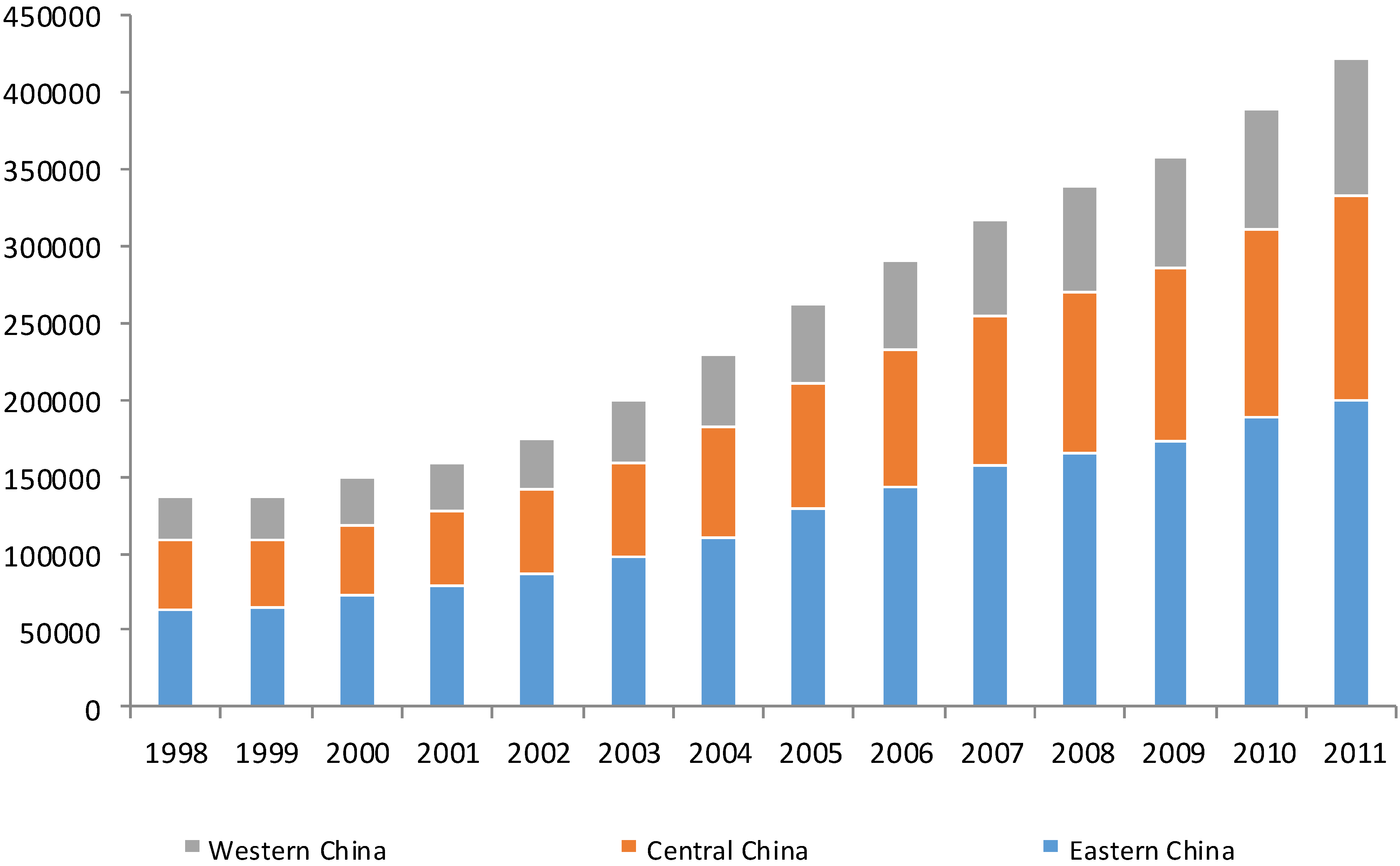
2.3. Energy Consumption in China

In addition to rapid economic growth in China since 1998, energy consumption also has also increasing dramatically during this time from 1.36 billion tons of standard coal in 1998 to 3.48 billion tons in 2011. This annual growth rate in energy consumption is 7.48 percent, which is only a little smaller than the GDP growth rate during this time. On a regional basis, Eastern China has the largest growth rate by energy consumption and is responsible for 46 percent of total energy consumption in China. Figure 1 below illustrates the regional growth in energy consumption across regions in China.

Figure 1. Energy consumption in China. Source: China Energy Statistical Yearbook [20].

Figure 1. Energy consumption in China. Source: China Energy Statistical Yearbook [20].

While growth in energy consumption has closely followed GDP growth in China, energy intensity has shown a downward trend during this same time period. Energy intensity is the ratio of energy consumption to GDP, which is a common index to describe energy utilization. Figure 2 illustrates the national and regional level trends in energy intensity in China. Energy intensity has decreased from 1.61 of 1998 to 1.19 of 2011, which means that the energy consumption to produce 10,000 RMB GDP has been reduced by 0.42 ton of standard coal in China. However, this downward trend was briefly interrupted from 2002 to 2005, a period that saw no significant reduction in energy intensity. This is because Chinese industrial development entered a new round of heavy industrial development during this period and the share of heavy industry’s gross output to total industry increased from 60.9% in 2002 to 69.5% in 2006. Although Eastern China is the biggest consumer of energy, it has also experienced the largest drop in energy intensity. This indicates that Eastern China consumes the least amount of energy to produce the same GDP as Western China and Central China. As showed in Figure 2, energy intensity has decreased in all regions in China but the gaps between the three regions have remained constant.

Figure 2. Energy intensity in China. Source: China Energy Yearbook and China Statistical Yearbook [20].

Figure 2. Energy intensity in China. Source: China Energy Yearbook and China Statistical Yearbook [20].

3. Results and Discussion

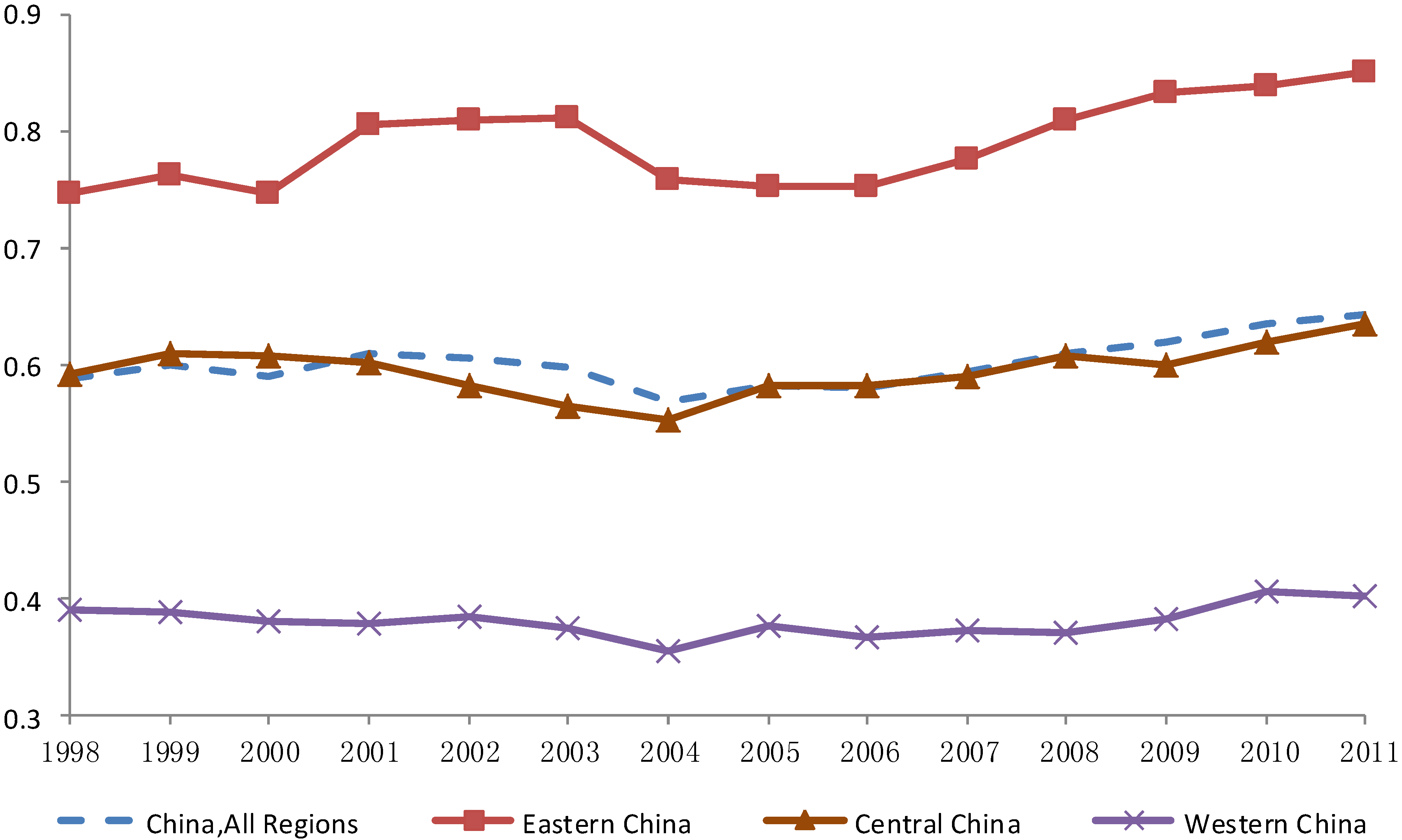
3.1. Energy Efficiency

For our analysis of energy efficiency in China, we use the definition of Hu and Wang [1], who define energy efficiency as the ratio of the optimal energy input to actual energy input. Figure 3 illustrates energy efficiency for China’s three regions (see Appendix C for a breakdown of provinces in each of the three regions). In 2011, overall energy efficiency in China is 0.64, but regionally Eastern China has the highest energy efficiency of 0.84 compared to 0.63 and 0.40 for Central and Western China, respectively. This indicates that actual energy inputs could be decreased by 36 percent for the whole of China and 16, 37 and 60 percent for Eastern, Central, and Western China, respectively, without a decrease in output. During the period 1998 to 2003, there is no significant improvement in energy efficiency at both the national and regional level. This is likely due to weak economic development following the Asia financial crisis in 1998.

After 2003, energy efficiency shows an obvious upward trend in China. This corresponds to several other trends. First, China’s economy began to grow rapidly again at this time. Second, stricter environmental regulations were enacted around this time. Finally, the service sector began to grow relative to other sectors at this time. Given the lower energy use and higher energy efficiency associated with the service sector, this could account for some of the growth in energy efficiency (see Appendix B for data on service sector growth in China). Regarding regional differences, Central and Western China show a slight increase in energy efficiency between 1998 and 2011, which closely follows the national trend. Eastern China shows the largest improvement in energy efficiency, well above the national trend. Interestingly, Eastern China also shows the largest growth in the service sector during this time, whereas Eastern and Central China’s service sector did now grow.

Figure 3. China’s regional energy efficiency (1998–2011).

Figure 3. China’s regional energy efficiency (1998–2011).

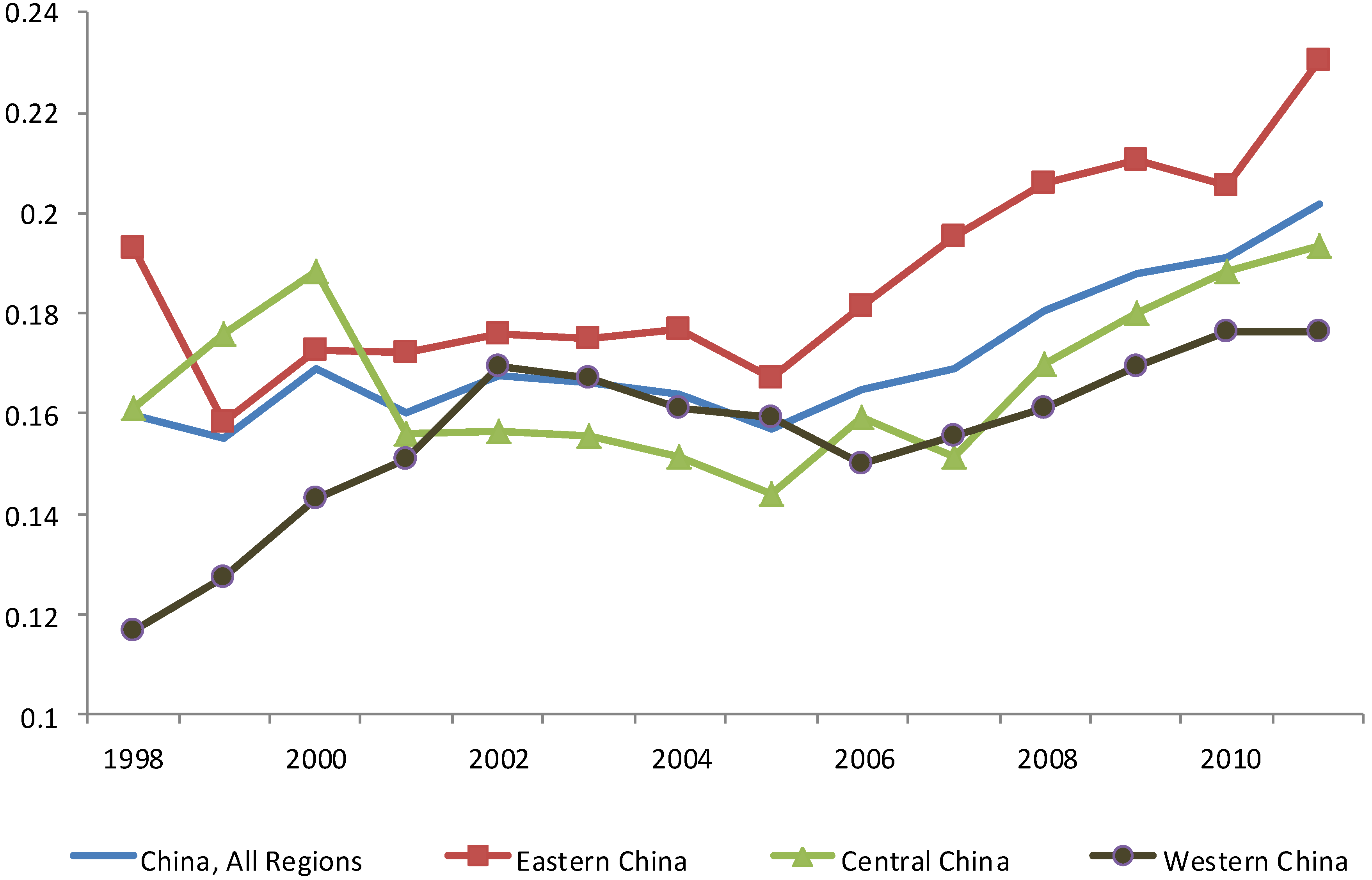
3.2. Shadow Price of Energy

Figure 4 below illustrates the trends in shadow prices across China as measured by our non-parametic methods. In the beginning of the sample period, the shadow price for energy is 0.1595, 0.1931, 0.1631 and 0.1167 for China overall, Eastern China, Central China, and Western China, respectively. These figures suggest that energy input can produce 1595 RMB, 1931 RMB, 1631 RMB and 1167 RMB with each additional energy input as measured by metric tons of standard coal when using 1998 shadow energy prices. However, using 2011 shadow energy prices the additional metric ton of standard coal can produce 2019 RMB, 2305 RMB, 1934 RMB and 1765 RMB. From 1998 to 2001, the shadow price in Western China shows rapid growth, but Eastern China and Central China show no obvious increase. Unlike energy efficiency in Figure 3, the shadow prices for the whole of China and the three main regions show no obvious upward trend from 2001 to 2005. This is contrary to the rapid GDP growth experienced during this same time period. However, following the implementation of stricter environmental regulations shadow prices start to rise in 2006 in all three regions in China. Another explanation for the impact of environmental regulation on shadow prices of energy may be the role of technology and new manufacturing equipment. Fujii et al. [22] find that investments in new manufacturing technology may reduce total factor productivity at least in the short-run, but if the goal is to increase productivity while minimizing undesirable outputs, such as CO₂ emissions from energy usage, then new manufacturing technology is highly effective. It may be the case that environmental regulations had the effect of encouraging investment in new manufacturing technologies.

Figure 4. China’s regional shadow price of energy.

Figure 4. China’s regional shadow price of energy.

In patterns similar to those shown in Figure 3, Eastern China also has a larger shadow price of energy input than Central China and Western China, and this indicates that Western China and Central China have worse energy utilization performance than Eastern China. Interesting, though, is the large increase in shadow prices in Western China from 1998 to 2002. This corresponds to a similar increase in the proportion of the service sector in Western China during the same time period (see Appendix B). Likewise, the largest growth in shadow prices after 2006 occurs in Eastern China, which also experienced growth in the service sector proportion of their economy after 2006.

Figure 5 below illustrates the ranking results of Chinese provincial shadow prices of energy input in 2011. Jiangsu, Hainan, Jiangxi, Fujian and Henan provinces have the best performance by the shadow price of energy, while the provinces with the lowest shadow price are Sichuan, Guangxi, Zhejiang, Ningxia and Anhui. Among the top performing provinces, Jiangsu, Hainan and Fujian are the provinces that belong to the Eastern regions with a higher level of economic development, but Jiangxi and Henan have lower levels of economic development and are located in Central China. Among the lowest performing provinces, Zhejiang is located in Eastern China, and the other low performing provinces are located in Western China and Central China. Thus, the shadow price of energy is not necessarily determined solely by higher economic development, but likely by other factors, such as industry structure, technological change, and resource endowments.

Figure 5. Chinese provincial shadow price of energy in 2011.

Figure 5. Chinese provincial shadow price of energy in 2011.

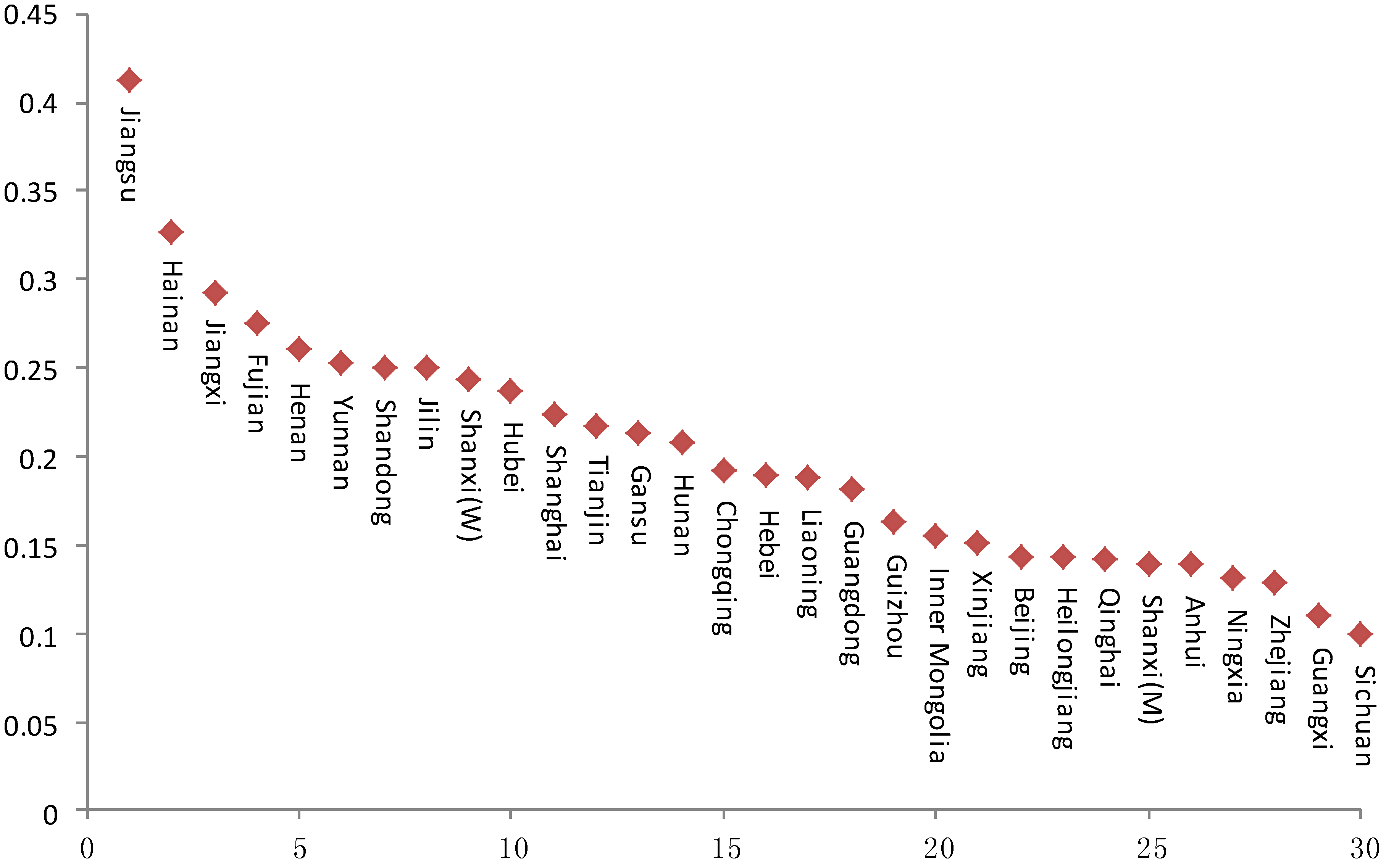
3.3. Shadow Price versus Market Price of Energy

Comparing the shadow price of energy input with energy efficiency, the shadow price of energy represents the marginal productivity of energy input under the given technology and energy efficiency as defined by Hu and Wang [1] presents the relative distance from the actual energy input to the optimal energy input with the assumption that all the provinces have the same technology and can reach the production frontier by resource allocation. However, every province has a diverse industrial structure, economic development level, and factor endowments. Thus, the assumption of identical technology across provinces would not be met. But the shadow price is the marginal productivity, which is computed without the assumption of identical technologies across provinces, and thus reflects provincial characteristics, such as industry structure and technology change. Thus we follow Khademvatani and Gordon [4] using the gap between the shadow price and the market price as the preferred method to measure the performance of energy.

As the market price of energy cannot be collected from official statistics in China, we use the retail price indices of fuel (REF) as the proxy variable for the change in the market price of energy. In order to capture the nominal change in the shadow price for energy, the GDP deflator is used to adjust the constant shadow price to be the current shadow price since the shadow price is measured by the additional GDP produced by the additional input of energy, and we use the ratio of the annual growth of shadow price to REF to describe the relationship between the shadow price and market price of energy. We then use a t-test for mean-comparison to analyze whether the shadow price is larger or smaller than the market price of energy.

Table 2 presents the ratio of the shadow price to the market price for energy for China’s thirty provinces. There are eighteen provinces whose shadow price is lower than the market price confirmed by the t-test, which suggests that the provinces could increase the marginal productivity and improve energy efficiency by a reallocation of energy input and other inputs. For the remaining twelve provinces, we cannot reject the null hypothesis that the shadow price is equal to the market price of energy, and thus these provinces may be at their Pareto-optimal levels of energy input. Regarding Table 2, some of the provinces whose shadow prices are equal to the market price for energy have higher levels of energy efficiency, such as Jiangsu, Tianjin, and Zhejiang. But there are also some provinces with shadow prices equal to the market price that have low energy efficiency, such as Chongqing and Sichuan. Even though the shadow prices of energy are equal to the market price in these provinces, their fast economic development relies heavily on the rapid growth of the second industry, which is a larger consumer of energy than other industries.

Table 2. Ratio of shadow price to market price for energy in China.

Province	1999	2001	2003	2005	2007	2009	2011	T (R < 1)	T (R ≠ 1)	T (R > 1)
Beijing	0.93	0.92	0.92	0.83	1.00	0.77	1.25	0.08	0.15	0.92
Tianjin	1.09	0.92	0.95	0.84	1.50	0.95	0.97	0.45	0.90	0.55
Hebei	1.06	0.93	0.93	0.81	1.04	1.02	0.97	0.01	0.01	0.99
Liaoning	0.28	0.06	1.10	0.95	0.99	0.94	1.53	0.88	0.24	0.12
Shanghai	1.03	0.89	1.00	0.88	1.03	1.02	1.00	0.02	0.04	0.98
Jiangsu	1.05	1.03	0.92	0.82	1.11	1.26	1.05	0.49	0.98	0.51
Zhejiang	0.95	1.03	0.93	0.86	1.02	1.10	1.42	0.21	0.42	0.79
Fujian	0.85	1.00	0.91	0.73	1.05	1.17	0.94	0.03	0.07	0.97
Shandong	1.06	0.89	0.95	0.81	0.99	1.02	0.99	0.01	0.02	0.99
Guangdong	1.01	1.03	0.90	0.84	1.00	1.08	0.81	0.01	0.01	0.99
Hainan	1.00	1.06	0.89	0.85	1.00	1.08	0.98	0.10	0.22	0.89
Shanxi	1.09	0.39	0.89	0.81	0.34	0.99	0.94	0.02	0.05	0.98
Inner Mongolia	1.28	1.00	1.01	0.81	1.05	1.00	1.00	0.19	0.39	0.81
Jilin	1.00	0.87	0.88	0.85	1.07	1.10	0.93	0.02	0.04	0.98
Heilongjiang	1.01	0.97	1.02	0.96	1.04	0.95	0.94	0.15	0.29	0.85
Anhui	1.09	1.03	0.99	0.31	1.09	0.94	0.80	0.65	0.70	0.35
Jiangxi	1.22	1.07	0.98	0.84	0.98	1.10	1.03	0.56	0.88	0.44
Henan	1.03	0.95	0.95	0.83	1.06	0.95	0.89	0.00	0.00	1.00
Hubei	1.06	1.04	0.92	0.87	1.08	1.12	0.96	0.15	0.30	0.85
Hunan	1.06	1.03	0.92	0.78	1.04	1.11	0.93	0.05	0.11	0.95
Guangxi	1.24	1.10	0.86	0.76	0.97	1.03	0.95	0.73	0.54	0.27
Chongqing	1.15	1.15	1.00	0.91	0.97	1.01	0.87	0.76	0.47	0.24
Sichuan	1.26	1.08	0.91	0.83	0.96	1.01	0.95	0.64	0.72	0.36
Guizhou	1.15	1.06	0.90	0.96	0.99	0.97	0.92	0.10	0.21	0.90
Yunan	1.04	1.04	0.96	0.82	1.05	0.92	0.97	0.05	0.09	0.95
Shannxi	1.18	0.98	0.93	0.84	0.99	0.96	0.95	0.07	0.15	0.93
Gansu	1.01	0.98	0.96	0.82	1.02	0.95	0.92	0.05	0.11	0.95
Qinghai	0.90	1.05	0.97	0.79	1.00	0.93	0.86	0.03	0.05	0.97
Ningxia	1.09	1.00	0.80	0.82	1.09	0.96	0.85	0.02	0.04	0.98
Xinjiang	1.07	0.89	1.00	0.87	0.96	0.93	0.83	0.08	0.16	0.92

Notes: T (R < 1) is the one tailed t-test for the alternative hypothesis of the shadow price being less than the market price, T (R ≠ 1) the two tailed test for the alternative hypothesis of the shadow price not equaling the market price, and T (R > 1) the one tailed t-test for the alternative hypothesis of the shadow price being greater than the market price. The value below each t-test is the p-value. For 18 provinces the shadow price is significantly lower than the market price. Highlighted in bold are the p-values for the 12 provinces where no significant difference between the shadow price and market price was found.

Table 2. Ratio of shadow price to market price for energy in China.

Province	1999	2001	2003	2005	2007	2009	2011	T (R < 1)	T (R ≠ 1)	T (R > 1)
Beijing	0.93	0.92	0.92	0.83	1.00	0.77	1.25	0.08	0.15	0.92
Tianjin	1.09	0.92	0.95	0.84	1.50	0.95	0.97	0.45	0.90	0.55
Hebei	1.06	0.93	0.93	0.81	1.04	1.02	0.97	0.01	0.01	0.99
Liaoning	0.28	0.06	1.10	0.95	0.99	0.94	1.53	0.88	0.24	0.12
Shanghai	1.03	0.89	1.00	0.88	1.03	1.02	1.00	0.02	0.04	0.98
Jiangsu	1.05	1.03	0.92	0.82	1.11	1.26	1.05	0.49	0.98	0.51
Zhejiang	0.95	1.03	0.93	0.86	1.02	1.10	1.42	0.21	0.42	0.79
Fujian	0.85	1.00	0.91	0.73	1.05	1.17	0.94	0.03	0.07	0.97
Shandong	1.06	0.89	0.95	0.81	0.99	1.02	0.99	0.01	0.02	0.99
Guangdong	1.01	1.03	0.90	0.84	1.00	1.08	0.81	0.01	0.01	0.99
Hainan	1.00	1.06	0.89	0.85	1.00	1.08	0.98	0.10	0.22	0.89
Shanxi	1.09	0.39	0.89	0.81	0.34	0.99	0.94	0.02	0.05	0.98
Inner Mongolia	1.28	1.00	1.01	0.81	1.05	1.00	1.00	0.19	0.39	0.81
Jilin	1.00	0.87	0.88	0.85	1.07	1.10	0.93	0.02	0.04	0.98
Heilongjiang	1.01	0.97	1.02	0.96	1.04	0.95	0.94	0.15	0.29	0.85
Anhui	1.09	1.03	0.99	0.31	1.09	0.94	0.80	0.65	0.70	0.35
Jiangxi	1.22	1.07	0.98	0.84	0.98	1.10	1.03	0.56	0.88	0.44
Henan	1.03	0.95	0.95	0.83	1.06	0.95	0.89	0.00	0.00	1.00
Hubei	1.06	1.04	0.92	0.87	1.08	1.12	0.96	0.15	0.30	0.85
Hunan	1.06	1.03	0.92	0.78	1.04	1.11	0.93	0.05	0.11	0.95
Guangxi	1.24	1.10	0.86	0.76	0.97	1.03	0.95	0.73	0.54	0.27
Chongqing	1.15	1.15	1.00	0.91	0.97	1.01	0.87	0.76	0.47	0.24
Sichuan	1.26	1.08	0.91	0.83	0.96	1.01	0.95	0.64	0.72	0.36
Guizhou	1.15	1.06	0.90	0.96	0.99	0.97	0.92	0.10	0.21	0.90
Yunan	1.04	1.04	0.96	0.82	1.05	0.92	0.97	0.05	0.09	0.95
Shannxi	1.18	0.98	0.93	0.84	0.99	0.96	0.95	0.07	0.15	0.93
Gansu	1.01	0.98	0.96	0.82	1.02	0.95	0.92	0.05	0.11	0.95
Qinghai	0.90	1.05	0.97	0.79	1.00	0.93	0.86	0.03	0.05	0.97
Ningxia	1.09	1.00	0.80	0.82	1.09	0.96	0.85	0.02	0.04	0.98
Xinjiang	1.07	0.89	1.00	0.87	0.96	0.93	0.83	0.08	0.16	0.92

Notes: T (R < 1) is the one tailed t-test for the alternative hypothesis of the shadow price being less than the market price, T (R ≠ 1) the two tailed test for the alternative hypothesis of the shadow price not equaling the market price, and T (R > 1) the one tailed t-test for the alternative hypothesis of the shadow price being greater than the market price. The value below each t-test is the p-value. For 18 provinces the shadow price is significantly lower than the market price. Highlighted in bold are the p-values for the 12 provinces where no significant difference between the shadow price and market price was found.

4. Conclusions and Policy Recommendations

Overall, our analysis of energy shadow prices and energy efficiency in China leads us to three main findings. First, based on the measure of energy efficiency proposed by Hu and Wang [9] we conclude that energy efficiency is at a low level in China and can be improved by reallocation of the energy input and other inputs. Energy efficiency does not show any substantial changes from 1998 to 2003 both in the whole China and the three main regions, but does show a significant increase after the stricter environmental policies were implemented after 2006. With regards to the gaps among the three main regions, Eastern China performs better than Central and Western China by energy efficiency, and the gaps between provinces show no obvious reduction during the sample period. These results are similar to prior studies, such as Hu and Li [1], Chang and Hu [23] and Wang and Feng [24], but show some differences with Zhang et al. [25] who takes undesirable outputs, such as carbon dioxide, sulfur dioxide emission and the chemical oxygen demand, into account.

Second, our results also indicate that shadow prices of energy experienced rapid growth after 2006 in both the whole of China and in the three main regions. This corresponds to a period of growth in energy efficiency during the same period. As for the provincial ranking of energy’s shadow prices, Jiangsu, Hainan, Jiangxi and Fujian have shadow prices close to market price, which corresponds closely with energy efficiency in their regions. However, other provinces, such as Henan and Shandong, have shadow prices close to market prices but low energy efficiency as measured by the ratio of the annual growth of energy’s shadow price to REF. Eighteen provinces have shadow prices lower than the market price for energy, which indicates that they can increase the marginal productivity of energy and improve energy efficiency through reallocation of inputs.

Finally, analysis of energy scarcity serves as an important basis for formulating national energy policy. More than half of the provinces have a lower shadow price than the market price, which suggests a degree of market failure in Chinese energy markets. Khademvatani and Gordon [4] suggest that changes in tax policy can help raise the shadow price of energy to move shadow prices closer with market prices. In addition to tax policy, environmental regulations may also improve energy efficiency. Our results show only a slight increase in energy efficiency after 2006 when stricter environmental regulations were enacted, but sharply rising shadow prices during this time. This indicates that environmental regulations may be more effective than previously believed, and overtime may lead to shadow prices more closely in line with market prices. In addition, we find that Eastern China experienced strong growth in both shadow prices and energy efficiency. This may be due to the relative growth of the service sector in Eastern China. This suggests that future efforts by policy makers to balance China’s economy away from heavy industry towards consumption and services may also lead to improved energy efficiency and a closer alignment between shadow prices and market prices of energy.

A promising area for future research would be to examine shadow prices at the industry level to further examine the relationship between service industries and shadow prices compared to other sectors. In addition, micro-level analysis of shadow prices and new manufacturing technologies would help further examine how environmental regulations after 2006 lead to increases in shadow prices across China. Finally, additional research should be done on shadow prices of energy both in rapidly developing economies, such as India, as well as highly developed economies with strong environmental protection laws, such as Western Europe or Japan.

References

1. Hu, J.L.; Wang, S.C. Total-factor energy efficiency of regions in China. Energy Policy 2006, 34, 3206–3217. [Google Scholar] [CrossRef]
2. Zhang, X.P.; Cheng, X.M.; Yuan, J.H.; Gao, X.J. Total-factor energy efficiency in developing countries. Energy Policy 2011, 39, 644–650. [Google Scholar] [CrossRef]
3. Chen, Z.C.; Lin, Z.S. Multiple timescale analysis and factor analysis of energy ecological footprint growth in China 1953–2006. Energy Policy 2008, 36, 1666–1678. [Google Scholar] [CrossRef]
4. Khademvatani, A.; Gordon, D.V. A marginal measure of energy efficiency: The shadow value. Energy Econ. 2013, 38, 153–159. [Google Scholar] [CrossRef]
5. Aigner, D.; Chu, S.F. On the estimating the industry production function. Am. Econ. Rev. 1968, 58, 226–239. [Google Scholar]
6. Schmidt, P. On the statistical estimation of parametric frontier production functions. Rev. Econ. Stat. 1976, 58, 238–239. [Google Scholar] [CrossRef]
7. Pitman, R.W. Multilateral productivity comparisons with undesirable outputs. Econ. J. 1983, 93, 883–891. [Google Scholar] [CrossRef]
8. Shephard, R.W. Theory of Cost and Production Functions; Princeton University Press: Princeton, NJ, USA, 1970. [Google Scholar]
9. Hailu, A.; Veeman, T.S. Environmentally sensitive productivity analysis of the Canadian pulp and paper industry, 1959–1994: An input distance function approach. J. Environ. Econ. Manag. 2000, 40, 251–274. [Google Scholar] [CrossRef]
10. Lee, M. The shadow price of substitutable sulfur in the US electric power plant: A distance function approach. J. Environ. Manag. 2005, 77, 104–110. [Google Scholar] [CrossRef]
11. Färe, R.; Grosskopf, S.; Lovell, C.A.K.; Yaisawarng, S. Derivation of shadow prices for undesirable outputs: A distance function approach. Rev. Econ. Stat. 1993, 75, 374–380. [Google Scholar] [CrossRef]
12. Färe, R.; Grosskopf, S.; Noh, D.; Weber, W. Characteristics of a polluting technology: Theory and practice. J. Economet. 2005, 126, 469–492. [Google Scholar] [CrossRef]
13. Murty, M.N.; Kumar, S.; Dhavala, K.K. Measuring environmental efficiency of industry: A case study of thermal power generation in India. Environ. Resour. Econ. 2007, 38, 31–50. [Google Scholar] [CrossRef] [Green Version]
14. Boyd, G.; Molburg, J.; Prince, R. Alternative methods of marginal abatement cost estimation: Nonparametric distance functions. In Proceedings of the 17th North American Conference of the International Association for Energy Economics, Boston, MA, USA, 26–30 October 1996; pp. 86–95.
15. Chung, Y.H.; Fare, R.; Grosskopf, S. Productivity and undesirable output: A directional distance function approach. J. Environ. Manag. 1997, 51, 229–240. [Google Scholar] [CrossRef]
16. Lee, J.D.; Park, J.B.; Kim, T.Y. Estimation of the shadow prices of pollutants with production/environment inefficiency taken into account: A nonparametric directional distance function approach. J. Environ. Manag. 2002, 64, 365–375. [Google Scholar] [CrossRef]
17. Ouyang, X.; Sun, C. Energy savings potential in China’s industrial sector: From the perspectives of factor price distortion and allocative inefficiency. Energy Econ. 2015, 48, 117–126. [Google Scholar] [CrossRef]
18. China Statistical Yearbook; Chinese Statistical Bureau: Beijing, China, 1998–2011.
19. Statistical Yearbook of the Chinese Investment in Fixed Assets; Chinese Investment Press: Beijing, China, 1998–2011.
20. China Energy Statistical Yearbook; China Statistics Press: Beijing, China, 1998–2011.
21. Zhang, J.; Wu, G.; Zhang, J. The estimation of China’s provincial capital stock: 1952–2004. Econ. Res. J. 2004, 10, 35–44. (In Chinese) [Google Scholar]
22. Hidemichi, F.; Shinji, K.; Shunsuke, M. Changes in environmentally sensitive productivity and technological modernization in China’s iron and steel industry in the 1990s. Environ. Dev. Econ. 2010, 15, 485–504. [Google Scholar] [CrossRef]
23. Chang, T.; Hu, J. Total-factor energy productivity growth, technical progress, and efficiency change: An empirical study of China. Appl. Energy 2010, 87, 3262–3270. [Google Scholar] [CrossRef]
24. Wang, Z.; Feng, C.; Zhang, B. An empirical analysis of China’s energy efficiency from both static and dynamic perspectives. Energy 2014, 74, 322–330. [Google Scholar] [CrossRef]
25. Zhang, N.; Kong, F.; Yu, Y. Measuring ecological total-factor energy efficiency incorporating regional heterogeneities in China. Ecol. Indic. 2015, 51, 165–172. [Google Scholar] [CrossRef]