Model Property Based Material Balance and Energy Conservation Analysis for Process Industry Energy Transfer Systems

Abstract

Conventional historical data based material and energy balance analyses are static and isolated computations. Such methods cannot embody the cross-coupling effect of energy flow, material flow and information flow in the process industry; furthermore, they cannot easily realize the effective evaluation and comparison of different energy transfer processes by alternating the model module. In this paper, a novel method for material balance and energy conservation analysis of process industry energy transfer system is developed based on model property. Firstly, a reconfigurable energy transfer process model, which is independent of energy types and energy-consuming equipment, is presented from the viewpoint of the cross-coupling effect of energy flow, material flow and information flow. Thereafter the material balance determination is proposed based on both a dynamic incidence matrix and dynamic balance quantity. Moreover, the model-weighted conservation determination theorem is proved, and the energy efficiency analysis method is also discussed. Results confirmed the efficacy of the proposed methods, confirming its potential for use by process industry in energy efficiency analyses.

1. Introduction

Model property analysis can be harnessed to reflect the characteristics of an existing system, and furthermore, such an approach can also be adopted in system design to help ensure the correct implementation of a new system [1]. An energy transfer process model, as the key sub-model of a process industry energy transfer system, embodies both behaviour and structure characteristics [2]. Analyzing the properties of the energy transfer process model can help evaluate and validate any practical system simulated by the model.

A process industry energy transfer system consists of energy-consuming units (for example, equipment) and the coupling relationship between units comprising the system [3]. Different equipment exhibit different working characteristics, so the models for equipment are diverse. Research concerning models of energy-consuming equipment is significant and has been predominantly based on the system identification modeling method [4,5,6]. However, most of this research only focuses on the energy saving of individual equipment; it neglects the issues of relationship and coordination between the different equipment that comprise an arbitrary system. Nevertheless, the coupling relationship between the different equipment determines the structure of the energy transfer system, and the upstream and downstream interaction; thus a process model reflecting the coupling relationship between the different constituent units is of crucial importance.

At present, common process modeling methods mainly include sequential modular approach, equation-oriented approach and simultaneous modular approach [7,8,9]. The sequential modular approach can easily solve the sequential structure process but cannot be well utilized for the simulation of a process with one or more loops because the process partitioning and cutting means must be adopted initially; this will increase the workload and difficulty of the simulation calculation [10]. The equation-oriented approach needs to establish the huge equations for a complex process [11]. Indeed, computational complexity is the primary drawback for both the equation-oriented approach and the simultaneous modular approach [12]. Moreover, the technological process of the process industry is complex and heterogeneous, and the material flow, energy flow and information flow are cross-coupled. How to promote the adaptability of the process model and meanwhile embody the coupling effect of these three different flows is an important issue. Although the various production processes differ with respect to energy type, energy-consuming equipment, materials, products, and so forth, they have in common the process characteristics of parallel, serial, bypass and reflux structures. Therefore, constructing a reconfigurable energy transfer process model, which not only can embody the coupling relationship between energy flow, material flow and information flow, but also can describe the interaction and logic relation between the key factors of the energy transfer process, is meaningful and indispensable for material flow and energy flow analyses of process industry energy transfer systems.

The energy flow, material flow and information flow all coexist in process industry energy transfer systems. Material flow reflects the processing and implementation procedure of the main material product, and energy flow drives the transformation of the material flow. So, the material flow and energy flow, which are the specific embodiments of the production process, determine the resource utilization and energy efficiency. Information flow signals and influences the behaviour of the energy flow and material flow, and also reflects the external environment information. The evolution state of the energy transfer system can be affected or changed by information regulating or external interventions such as the equipment startup/stop. Moeller et al. [13], using Petri nets, researched the simulation of material flow, focusing exclusively on pure material factors such as material input and output, but neglecting the cross-impact of energy, material, information, operator and so forth. Although the material flow and energy flow enter the process or equipment simultaneously, on the output side, there is the material flow along with energy outputs on account of the interaction of energy flow and material flow inside the equipment [14]. Only by comprehensively considering the coupling and separation effect between energy and material to research the energy transfer process can the integration and coordination of energy flow and material flow be properly understood and realized. Other researchers have investigated the mass and energy flow models for steel plant based on historical data, and analyzed the influences of enterprise energy structures in different technological processes, for example in [15,16]. Here, the researchers analyzed the energy consumption using static matching approaches; however such approaches cannot reflect the dynamic changes of energy. Furthermore, when the industry structure and technical factors are changed, methods based on historical data cannot be easily and effectively applied. As a result of being confined by isolated mass balance and thermal equilibrium, much conventional research on energy flow and material flow is static and insular. Research on process industry material and energy flow must be based on the concepts of energy transfer process networking and dynamic behaviour [2,17]. Therefore, research presented in this paper is based on the model of energy transfer process, and the behaviour and structure properties of that model.

So far, taking advantage of graphic description, efficiently computation, as well as the concurrent, asynchronous and resource sharing modeling ability of Petri nets [18], the application of Petri nets and extended Petri nets in manufacture modeling and control is prevalent [19,20]. As the process industry is a continuous process along with discrete events, we have explored the fuzzy Petri net with hybrid behavior states and applied it to construct a model of an energy-consuming network including energy and non-energy flow between the different workshops [21,22]. This paper, in view of the characteristics of product heterogeneity, uncertainty and continuity of the process industry, firstly constructs the Reconfigurable Process Model of Process Industry Energy Transfer System (RPM_PIETS) from the perspective of comprehensively considering the inherent coupling effects of material, energy and information flows. Based on the semantics of the RPM_PIETS model, the dynamic and structure properties of the model can then be defined, and the material balance and energy conservation analysis of the process industry can be realized based on model properties.

Due to the RPM_PIETS model being developed by improving and extending fuzzy Petri nets in view of the particular modeling demands of process industry energy transfer processes, the analysis methods for RPM_PIETS are different from that of general Petri nets. At present, network analysis methods mainly include the algebraic analysis technique based on state equations, the diagram analysis method based on coverability tree, as well as the inductive analysis method based on decomposition and reduction [23,24]. The algebraic analysis technique, firstly proposed by Peterson [25], describes the net system as an incidence matrix and builds the linear relationship with state reachability. Murata [26] showed the properties of Petri nets, especially structure properties such as conservativeness, repetitiveness and so on, based on the relevant results of algebraic analysis. But this method cannot describe the dynamic characteristics adequately. The diagram analysis method with reachability tree reveals the dynamic running mechanism of a system by the finite directed tree, just like the state machine, but the complexity of the states of the complex system is unacceptable [27,28]. In order to avoid the analytical difficulty incurred by the state complexity of Petri nets, the inductive analysis method was presented according to the concepts of decomposition and reduction, and crucially, the original properties will still be retained during decomposition and reduction [29,30,31].

From the above discussion, the current model analysis methods have their own characteristics, but there are still certain application limitations and adaptability constraints. As the process industry energy transfer system has the distinct characteristics of continuity, uncertainty, concurrency and asynchronism, RPM_PIETS model is proposed with these characteristics being paramount. When analyzing the material balance and energy conservation of the process industry energy transfer process, this must be based on the semantics of the RPM_PIETS model. Because the normal incidence matrix cannot describe the dynamic features of the model, the respective concepts of static and dynamic incidence matrices are developed. In terms of dynamic and static incidence matrices, the RPM_PIETS model properties are researched, and the material balance analysis is conducted based on dynamic balance quantity. And then, based on an analysis of the model-weighted conservation, the energy conservation calculation of process industry energy transfer system is proposed.

The remainder of this paper is structured as follows: in Section 2, we introduce the formal specification of the reconfigurable process model of process industry energy transfer system after analyzing the key factors and their interactive relations which comprise process industry energy transfer process. In Section 3, we contribute the material balance analysis method based on model dynamic properties; related material balance and material overstock determination are put forward. Next, Section 4 presents the judgment theorem of model-weighted conservation, and describes the energy conservation and energy efficiency analysis for process industry energy transfer process. In Section 5, the validation experiment is presented after which the paper is concluded.

2. Reconfigurable Process Model of Process Industry Energy Transfer System

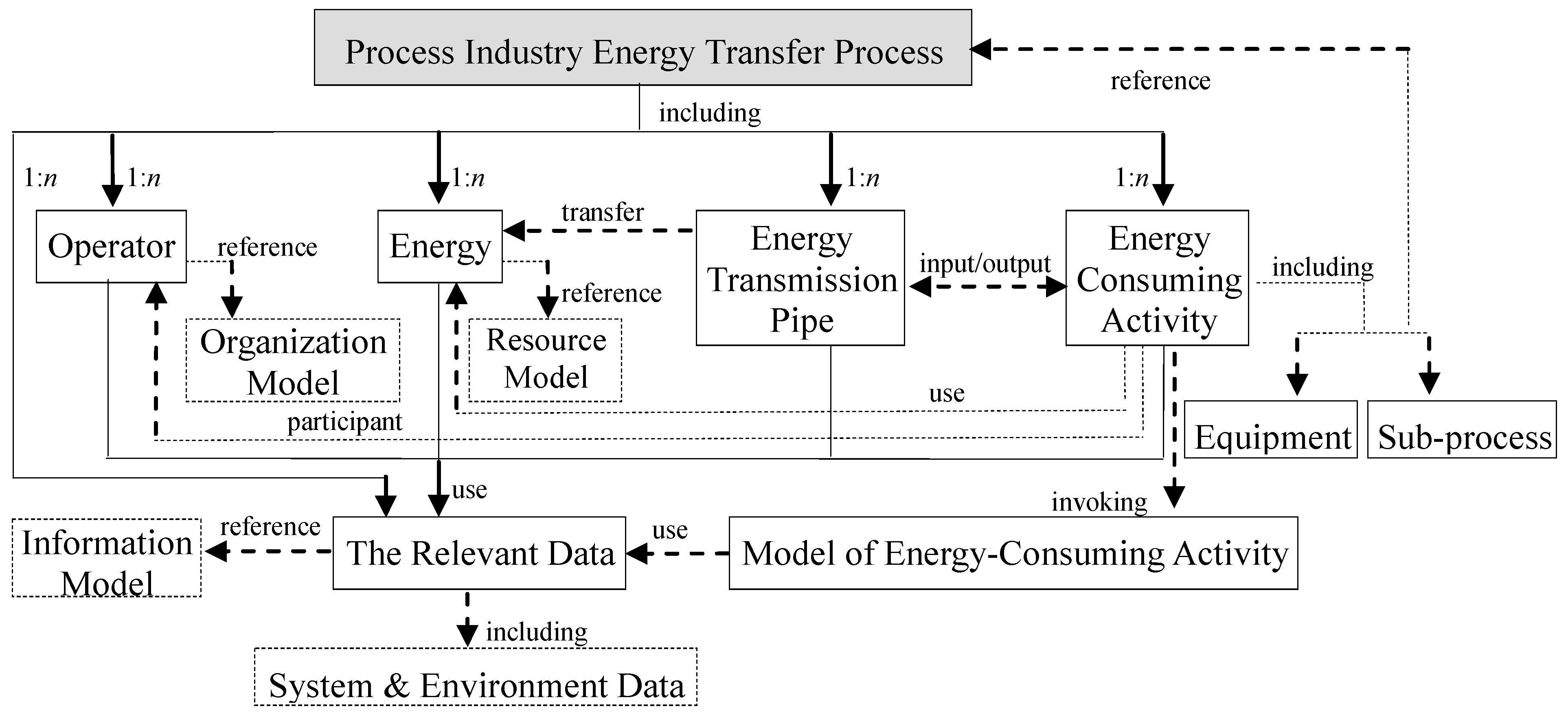
2.1. Key Factors and Interactive Relations

Different process industries differ in terms of technological processes, energy-consuming equipment and energy types; nonetheless, there still exists commonalities from the perspective of energy transfer processes. For example, all of the energy transfer processes not only consume the primary energy sources, but also consume the secondary energy sources and the energy-consumed medium, which are all energy carriers; additionally, the energy flow, material flow and information flow all coexist in the energy transfer process, and the enterprise personnel, management and other multiple factors, either individually or in combination, can affect the energy transfer process in the process industry.

To derive the common factors in energy transfer processes, it is necessary to extract the key factors in every aspect of energy transfer processes. The interior factors include energy intensity, energy transmission pipe loss rate, and so forth; the external factors that interact with the energy transfer process include external computation and control, personnel, and so forth. The key factors and interactive relations of the process industry energy transfer process are outlined in Figure 1. In the subsequent section, the reconfigurable process model of process industry energy transfer system is given in terms of Figure 1.

Figure 1. The key factors of process industry energy transfer process.

Figure 1. The key factors of process industry energy transfer process.

2.2. Formal Specification of Reconfigurable Energy Transfer Process Model

Energy transfer behaviour in the process industry is normally continuous; however, discrete events also occur in production processes. The various energy and non-energy materials flow through the equipment with the characteristics of concurrency and asynchronism. Thus, the modeling method for process industry energy transfer process must be process-centric, capable of describing both certain and uncertain information, and support highly effective analyses. In order to realize the behaviour and structure description of an enterprise energy transfer process, a fuzzy Petri nets model oriented to enterprise energy consumption process was explored [21]. Here, the Reconfigurable Process Model of Process Industry Energy Transfer System (RPM_PIETS) is further presented in view of energy flow, material flow and information flow.

Definition 1: A Reconfigurable Process Model of Process Industry Energy Transfer System (RPM_PIETS) is a 7-tuple: RPM_PIETS = (P, T, G, I(P,T), O(P,T), M₀(P), ∑). Every element of RPM_PIETS is formally defined as below.

Element 1: P

$P=\{P_1,P_2,\mathrm{...},P_n\}=P^C\cup P^D$ is a finite non-empty set of fuzzy places. Here, P^C denotes the set of continuous fuzzy places, which indicates the storehouses of process industry energy and non-energy materials or the warehouses of products. Here, the symbol “◎” represents P^C. P^D, denoting the set of discrete fuzzy places, indicates the information set such as the message and equipment state. Here, the symbol “○” represents P^D. For $\forall P_i\in P$, the detailed definition for the fuzzy place P_i is shown in Definition 2.

Element 2: T

$T=\{T_1,T_2,\mathrm{...},T_m\}=T^C\cup T^D$ is a finite nonempty set of fuzzy transitions, $P\cap T=\text{φ}$ and $P\cup T\ne \text{φ}$. Here, T^C denotes the set of continuous fuzzy transitions, which represents the energy-consuming activities or equipment, and T^C is symbolized by “□”. T^D denotes the set of discrete fuzzy transitions, which represents the logic control or message delivery in process industry energy transfer processes such as the start or stop operation for equipment, and T^D is symbolized by “▌”. For $\forall T_j\in T$, the fuzzy transition T_j is defined further in Definition 3.

Element 3: G

G={G₁,G₂, …, G_k} is a finite set of logic gates. $\forall G_j\in G$ is related to the input-output control of the fuzzy transition, and represents the join or split valves in the energy transmission pipe net. It can control the flowing directions of different input-output material, energy and information flows, and reflect the logic behaviour of concurrence or asynchrony and so forth in the energy transfer process. Here, it is symbolized by “Δ” in different directions in view of the input or output control gate.

Element 4: I(P, T)

$I(P,T)$ is a weighted fuzzy relation about $P\times T$. It shows the connectivity from fuzzy places to fuzzy transitions. For $\forall P_i\in P，\forall T_j\in T$, the rated input from P_i to T_j is defined as ${\text{λ}}_{i,j}$, the fuzzy link strength is defined as ${\text{ω}}_{i,j}$ and the input weight function can be as $I(P_i,T_j)$. In the model of the energy transfer process, the function $I(P_i,T_j)$ and ${\text{ω}}_{i,j}$ can be defined differently in view of the actual requirement. For example, when ${\text{ω}}_{i,j}$ represents the maximum transfer rate from P_i to T_j, let $I(P_i,T_j)=\text{min}\left\{{\text{λ}}_{i,j},{\text{ω}}_{i,j}\right\}$; when ${\text{ω}}_{i,j}$ represents the transmission loss rate from P_i to T_j, let $I(P_i,T_j)={\text{λ}}_{i,j}\times {\text{ω}}_{i,j}$ indicating the energy consumption in the transmission pipe.

Element 5: O(P, T)

O(P, T) is a weighted fuzzy relation about T × P. It shows the connectivity from fuzzy transitions to fuzzy places. For $\forall P_i\in P,\forall T_j\in T$, the rated output from T_j to P_i is defined as ${\text{λ}}_{i,j}$, the fuzzy link strength is defined as ${\text{ω}}_{i,j}$ and the output weight function is $O(P_i,T_j)$. The definition of function O(P_i, T_j) is similar to I(P_i, T_j).

Element 6: M₀(P)

M₀(P) denotes the initial marking set of fuzzy places and is the set valued on $[0,\infty ]$. It can reflect the initial resource allocation in the energy transfer process.

Element 7: ∑ = (E, Q, Π)

∑ = (E, Q, Π) is the set of auxiliary information. Here, E is the external event set, and Q is the set of external computing models and could reflect the working characteristic of the energy-consuming equipment. For example, Q is the set of mathematical models of energy-consuming activities, by which the product or semi-product output can be computed under a given energy input. Π is the set of relevant personnel information.

Definition 2: For $\forall P_i\in P$, the fuzzy place P_i is defined as $P_i=(M_0(P_i),M_i(t),d_i,K_i)$.

Where, M₀(P_i) denotes the initial marking or resource allocation of fuzzy place P_i. $\forall P_i\in P^C,M_0(P_i)\ge 0$; $\forall P_i\in P^D,M_0(P_i)\in N$ (N denotes non-negative integer). $M_i(t):P_i\to R^{+}\cup \left\{0\right\}$ is a mapping that denotes the marking of fuzzy place P_i at time t, which reflects the quantitative variation of the marking of fuzzy place P_i with time. At any time, $M_i(t)=M_i^r(t)+M_i^n(t)$, where $M_i^r(t)$ denotes the reserved marking of P_i that can’t enable other fuzzy transitions at time t. $M_i^n(t)$ denotes the non-reserved marking of P_i that can enable the related fuzzy transitions at time t.

d_i is the time limit associated with the fuzzy place P_i.

$K_i:P_i\to R^{+}$ ($R^{+}$ denotes the positive real) is the maximum capacity of P_i.

Definition 3: For $\forall T_j\in T$, the fuzzy transition T_j is defined as $T_j=({\text{τ}}_j,f_j,q_j,e_j,R_j,G_j,P{O}_j,N_j,d_{Tj},v_j(t))$.

Where, ${\text{τ}}_j:T_j\to R^{+}\cup \left\{0\right\}$ indicates the enabling threshold of T_j. In RPM_PIETS model, it specifies the indispensable minimum energy or materials required to enable the equipment to begin working.

f_j is the control function for the state changing of T_j. If $f_j\ge {\text{τ}}_j$, then the fuzzy transition T_j may be enabled. Generally, f_j is a non-negative function of the input weight function $I({}^{*}{T}_j,T_j)$; here ${}^{*}{T}_j$ denotes the preposition fuzzy place set of T_j.

$q_j$ is the mathematical or rule model for T_j and $q_j\in Q$. It reflects the dynamic characteristic of the energy-consuming activity or equipment. According to $q_j$, the output of the product or semi-finished product of equipment can be computed after the relevant physical and chemical reaction.

$e_j\in E$ is the external event associated with T_j, such as special information release, the occurrence of particular events or other typical external events, and so forth.

$R_j=({\text{ε,π}}_j)$, where $\text{ε}$ denotes the operating mode of T_j, $\text{ε}=\{\begin{array}{l}0,\text{\hspace{1em}automatic mode}\\ 1,\text{\hspace{1em}manual mode}\\ 2,\text{\hspace{1em}man-machine interactive mode}\end{array}$, and ${\text{π}}_j\in \text{Π}$ associates with the operator of T_j, if $\text{ε}=0$, ${\text{π}}_j=null$.

$G_j$ is the logic control gate of T_j and $G_j\in G$ as mentioned in Definition 1 (where G_j = IG_j and G_j = OG_j respectively denote the input and output logic control gate of T_j). It fulfills the role of routing management for information flow and energy or non-energy flow, and reflects the logic behaviour of concurrence or asynchrony, etc. It is related to the input-output control of the fuzzy transition T_j, and represents the join or split valves in the energy transmission pipe net.

$P{O}_j=IP{O}_j\cup OP{O}_j$ is the set of input and output fuzzy places of T_j. Here, $IP{O}_j\subset P$ is the input fuzzy places. If IG_j is the AND gate, $IP{O}_j={}^{*}{T}_j$ (${}^{*}{T}_j$ denotes the preposition fuzzy place set of T_j); If IG_j is the XOR gate, $IP{O}_j\subset {}^{*}{T}_j$. Contrarily, $OP{O}_j\subset P$ is the output fuzzy places of T_j. If OG_j is the AND gate, $OP{O}_j={T_j}^{*}$ (${T_j}^{*}$ denotes the postposition fuzzy place set of T_j); if OG_j is the XOR gate, $OP{O}_j\subset {T_j}^{*}$.

$N_j=(l,\int )$, where l denotes the hierarchy of T_j, $l=\{\begin{array}{l}0,T_j\text{ is atomic}\\ 1,T_j\text{ is abstract or hierarchy}\end{array}$, if l = 1, then $\int \in {\text{RPM\_PIET}}_{\text{S}}$ (RPM_PIETS_S is the subnet of RPM_PIETS).

For $T_j\in T^D$, $d_{Tj}$ is the firing delay, which generally describes the firing duration time of the discrete transition.

For $T_j\in T^C$, because the instantaneous firing speed of T_j is affected by both the material and energy supplies and the uncertain factors, from the viewpoint of uncertain factors, the instantaneous firing speed of T_j is defined as triangular fuzzy number. Here, ${\tilde{v}}_j=(v_j^l,v_j^n,v_j^m)$ is a triangular fuzzy number and denotes the instantaneous firing speed. $v_j^m$ is the maximum firing speed of T_j under the ideal working condition and $v_j^m=1/d_{T_j}$. $v_j^n$ is the rated firing speed which is restricted by the equipment production capacity and the material and energy transmission rate. $v_j^l$ is the minimum firing speed of T_j. At any time t, the actual firing speed of T_j is $v_j(t)$, and $v_j(t)=E({\tilde{v}}_j(t))=((1-\text{λ})v_j^l(t)+v_j^n(t)+\text{λ}{v}_j^m(t))/2$. Here, $v_j(t)$ is the expected value of the triangular fuzzy number ${\tilde{v}}_j(t)$, and $0\le \text{λ}\le 1$, $\text{λ}$ can be valued according to the risk attitude of experts and $\text{λ}=0.5$ means risk neutrality. If comprehensively considering several uncertain factors, ${\tilde{v}}_j(t)$ can be dynamically computed based on the triangular fuzzy number multi-attribute decision making method [32].

3. Material Balance Analysis Based on Model Dynamic Properties

3.1. Dynamic Incidence Matrix

An incidence matrix can reflect the net topology of the model in the algebraic analysis technique. For the RPM_PIETS model, due to the existence of the logic control gate as AND along with OR, and the dynamic changes of input and output intensity between energy supplier (fuzzy place) and energy-consuming equipment (fuzzy transition), the logical relation of material flows is different at different time and it changes dynamically.

Definition 4: Let $W(t)=W^{+}(t)-W^{-}(t)$, where $W_{j,i}^{-}(t)=I(P_i,T_j)$ represents the actual input intensity at time t from fuzzy place P_i to fuzzy transition T_j; its value will change according to the enabling condition of fuzzy transition T_j and the marking of fuzzy place P_i. As such, it will change dynamically. $W_{j,i}^{+}(t)=O(P_i,T_j)$ represents the actual output intensity at time t from fuzzy transition T_j to fuzzy place P_i, and its value will also change according to the operating mechanism of T_j; here, $i=1,2,\cdots ,n$; $n=\left|P\right|$; $j=1,2,\cdots ,m$; $m=\left|T\right|$. $W_{m\times n}(t)$ is defined as the dynamic incidence matrix, and its matrix element is $W_{j,i}(t)=W_{j,i}^{+}(t)-W_{j,i}^{-}(t)$.

It can be seen from the above Definition 4 that the dynamic incidence matrix reflects the running logical relation between different model nodes at some point, and embodies the flow direction of energy flow and material flow, as well as the logical connections of parallel, series, convergence and divergence and so on. The value of the dynamic incidence matrix element is a positive real number or zero.

3.2. Material Balance Determination Based on Dynamic Balance Quantity

In RPM_PIETS model, the marking of the fuzzy place is a function of time and fuzzy transition firing speed, and all the enabled fuzzy transitions will be fired simultaneously. Therefore, the traditional reachability tree method is difficult to be used when analyzing of RPM_PIETS model. Based on the above definition of the dynamic incidence matrix, the dynamic balance quantity which can reflect the quantitative change of energy storehouse or production warehouse is defined below.

Definition 5: In view of the dynamic incidence matrix of RPM_PIETS $W(t)={[W_{j,i}(t)]}_{m\times n}={[W_{j,i}^{+}(t)]}_{m\times n}-{[W_{j,i}^{-}(t)]}_{m\times n}$, for any continuous fuzzy place P_i, let:

$$B_i(t)={\displaystyle \sum _{j=1}^m{v}_j(t)}{W}_{j,i}^{+}(t)-{\displaystyle \sum _{j=1}^m{v}_j(t)}{W}_{j,i}^{-}(t)$$

(1)

where $v_j(t)$ is the instantaneous firing speed of the continuous fuzzy transition. For any discrete fuzzy place P_i, let:

$$B_i(t)={\displaystyle \sum _{j=1}^m{\text{σ}}_j(t)}{W}_{j,i}^{+}(t)-{\displaystyle \sum _{j=1}^m{\text{σ}}_j(t)}{W}_{j,i}^{-}(t)$$

(2)

where ${\text{σ}}_j(t)$ represents the firing state of the discrete transition; let $B(t)=[B_1(t),B_2(t),\cdots ,B_n(t)]$ and $B_i(t)$ is defined as the dynamic balance quantity of fuzzy place P_i at time t, and $B(t)$ is defined as the dynamic balance quantity of fuzzy place set of the model at time t.

Assuming that $[t,t+dt]$ is the operating range, so $M_i(t+dt)$ as the marking of fuzzy place P_i at time $t+dt$ can be deduced by $M_i(t)$, through the formula $M_i(t+dt)=M_i(t)+B_i(t)dt$, namely:

$$\frac{d{M}_i(t)}{dt}=B_i(t),i=1,2,\cdots ,n;n=\left|P\right|$$

and then $\frac{dM(t)}{dt}=B(t)$.

According to the Equation $\frac{dM(t)}{dt}=B(t)$, we can find that the dynamic balance quantity can reflect the input and output quantitative balance of the various warehouses of energy, material or production in the whole net system at any time. $B_i(t)$ reflects the instantaneous quantitative change of the warehouse P_i, whereby we can get the following inference:

If keeping $B_i(t)<0$ for a period of time, it means the material in the warehouse P_i will gradually diminish, representing a shortage in practice.

If keeping $B_i(t)>0$ for a period of time, it means the material in the warehouse P_i will gradually increase, representing an overstock in practice.

If keeping $B_i(t)$ in a steady periodic variation around zero coordinates, the material in the warehouse P_i can be kept in balance, avoiding an inadequate or excessive material supply.

3.3. Material Overstock Analysis Based on Boundedness

Definition 6: For $\forall P_i\in P$, if there is a non-negative real number L that makes $\forall M(t)\in \left\{M\right|\exists t\ge 0,M(t)=M\}$ and $M_i(t)\le L$, the fuzzy place $P_i$ is bounded, and $\underset{t\in [0,+\infty )}{\text{sup}}\{M_i(t)\}$ is the boundedness of the fuzzy place $P_i$, namely $L(P_i)=\underset{t\in [0,+\infty )}{\text{sup}}\{M_i(t)\}$; if every fuzzy place $P_i\in P$ is bounded, the RPM_PIETS model is bounded and $\text{max}\{L(P_i)|P_i\in P\}$ defines the boundary value.

Theorem 1: For $\forall P_i\in P$, let $B_i(t)$ represent the dynamic balance quantity of the fuzzy place $P_i$ at time $t$; if at any time $t$, there is always $B_i(t)\le 0$, the fuzzy place $P_i$ will definitely be bounded.

Proof: For $\forall P_i\in P$, the marking of $P_i$ at time $t$ is $M_i(t)$. According to Equation (3), we can get $\frac{d{M}_i(t)}{dt}=B_i(t)$, $t\ge 0$, thereby ${\displaystyle {\int }_0^t\frac{d{M}_i(t)}{dt}}dt={\displaystyle {\int }_0^t{B}_i(t)}dt$, that is $M_i(t)-M_i(0)={\displaystyle {\int }_0^t{B}_i(t)}dt$, $t\ge 0$. Because $M_i(t)\le M_i(0)$ can be deduced with $B_i(t)\le 0$, the fuzzy place $P_i$ is bounded.

If the maximum capacity, K_i, is defined for the fuzzy place P_i in the model RPM_PIETS, it can ensure the boundedness of P_i during the running of the RPM_PIETS model under the enabling rule.

The model boundedness can help to analyze whether there is production or material overstock under the initial material allocation scheme, and test for bottlenecks in the production process.

4. Energy Conservation Analysis Based on Model-Weighted Conservativeness

4.1. Energy Carrier and Energy Conservation

There exists energy and non-energy materials, such as primary energy, secondary energy, energy-consumed medium and diverse raw materials and products and so on. Primary energy refers to the natural and unprocessed energy resources, such as coal, natural gas, and water amongst others. Secondary energy, in order to meet the requirements of production, is transformed directly or indirectly from primary energy, such as electricity, all kinds of oil products, coal gas and so forth. The energy-consumed medium specifies that kind of working material which is not being used as raw material and not entering the product, but which must consume energy when forming itself. Moreover, all kinds of finished products and semi-finished products are made from primary energy, secondary energy and energy-consumed medium. Whatever energy and non-energy materials, there is an equivalent energy value corresponding to each of them. The equivalent energy value of the secondary energy material refers to the amount of the primary energy consumption during producing a unit quantity of the secondary energy. The equivalent energy values of the energy-consumed medium and all kinds of productions also mean the amount of the primary energy consumption during producing a unit quantity of the energy-consumed medium or production. Therefore, each kind of energy can be converted into the equivalent tons of standard coal.

It can be seen that whatever primary energy, secondary energy, energy-consumed medium and diverse raw materials and products, they are all energy carriers and can be transformed or produced by consuming primary energy. So, the analysis for process industry energy transfer system should be executed based on the total energy consumption. For the overall energy transfer system, no matter where and what the energy flows and converts, there exists the characteristic of energy conservation in the whole system. This means all the energy consumed in the production process can be regarded as being transferred to the different productions. So, all of the inputted energy and materials for the equipment can be converted into the supplied energy; all the output products of the equipment can be converted into the effective energy; All the emission waste of the equipment can then be converted into the loss energy.

According to the above idea, the determination method of model-weighted conservation is presented in this section. Through the calculation of energy conservation weighted matrix, the comprehensive energy consumption and the energy efficiency of equipment and production in the process industry are analyzed. In this section, the definitions of the static incidence matrix and the model-weighted conservation are respectively given at first; one kind of model-weighted conservation calculation based on S-invariant is then proposed.

4.2. Static Incidence Matrix

The static topology structure of a process industry energy transfer process can be reflected by a static incidence matrix, and the system structure properties depend on the network topology structure. Thus, the definition of the static incidence matrix is also indispensable to the analysis of RPM_PIETS model.

Definition 7: Let $C=C^{+}-C^{-}$, where $C_{j,i}^{-}:P_i\times T_j\to \{0,\begin{array}{c}\end{array}1\}$ denotes whether there exists a connection between fuzzy place P_i and fuzzy transition T_j. If the connection exists, $C_{j,i}^{-}=1$, otherwise $C_{j,i}^{-}=0$. $C_{j,i}^{+}:T_j\times P_i\to \{0,\begin{array}{c}\end{array}1\}$ denotes whether there exists a connection between fuzzy transition T_j and fuzzy place P_i. If the connection exists, $C_{j,i}^{+}=1$, otherwise $C_{j,i}^{+}=0$; $i=1,2,\cdots ,n$; $n=\left|P\right|$; $j=1,2,\cdots ,m$; $m=\left|T\right|$. $C_{m\times n}$ can be referred to as the static incidence matrix of the RPM_PIETS model, and the matrix element $C_{j,i}=C_{j,i}^{+}-C_{j,i}^{-}$. Here, $C^{-}$ is the output static incidence matrix, and $C^{+}$ is the input static incidence matrix.

Based on the static incidence matrix and the literature [29], the S-invariant can be defined as follows:

Definition 8: If and only if $C_{m\times n}\cdot I_{n\times 1}=0$, $m=\left|T\right|$, $n=\left|P\right|$ and any element of vector I is a non-negative real number, this $n\times 1$ vector I is the S-invariant of a RPM_PIETS model.

4.3. Model-Weighted Conservation Determination

Definition 9: For a RPM_PIETS model, if there exists one $n(n=|P|)$ dimensional weighted vector $I={[I(1),I(2),\cdots ,I(n)]}^T$, $\forall I(i)\in R^{+}$ , $i=1,2,\cdots ,n$, such that for any initial marking set $M_0$ of RPM_PIETS and $\forall M(t)\in \left\{M\right|\exists t\ge 0,M(t)=M\}$, there always exists ${\displaystyle \sum _{i=1}^n{M}_i}(t)I(i)={\displaystyle \sum _{i=1}^n{M}_i}(0)I(i)$, namely $M(t)I=M_{0}I$, So we can regard that RPM_PIETS as weighted conservation.

Theorem 2: If and only if the static incidence matrix $C$ of RPM_PIETS model satisfies $\left|C{C}^T\right|\ne 0$, the RPM_PIETS model is weighted conservation and the weighted matrix is S-invariant $I$.

Proof: On the basis of dynamics incidence, the marking of RPM_PIETS at any time can be calculated by the following Equation (4):

$$M(t)=M(t-dt)+[\text{σ}(t)+{\displaystyle {\int }_{u=t-dt}^{t}v(u)du]}W(t-dt)$$

(4)

Here, $M(t)$ and $M(t-dt)$ respectively represent the marking set of RPM_PIETS at current time and last time, and dt is the simulation step; $W(t-dt)$ is the dynamic incidence matrix during the running range $dt$. $\text{σ}(t)$, the simultaneous component with the continuous fuzzy transition is zero, reflects the firing situation of every discrete fuzzy transition between the last time $t-dt$ and the current time t. The component of v(u) represents the instantaneous firing speed of the associated continuous fuzzy transition, and the simultaneous component with the discrete fuzzy transition is zero.

From Definitions 4 and 7, it can be known that the static incidence matrix C and the dynamic incidence matrix W(t) are same type of matrix. At any time t, if there exists $X_t$ such that $X_t\cdot C=W(t)$, we can derive Equation (5) in terms of Equation (4).

$$M(t+dt)=M(t)+[\text{σ}(t+dt)+{\displaystyle {\int }_{u=t}^{t+dt}v(u)du]}W(t)=M(t)+[\text{σ}(t+dt)+{\displaystyle {\int }_{u=t}^{t+dt}v(u)du]}{X}_{t}C$$

(5)

Here, if $X_t\cdot C=W(t)$, $X_t\cdot (C{C}^T)=W(t)C^T$, and then $X_t\cdot (C{C}^T){(C{C}^T)}^{-1}=W(t)C^T{(C{C}^T)}^{-1}$.

Thereby, the solvable condition for equation $X_t\cdot C=W(t)$ is that the inverse of the square matrix $C{C}^T$ can be found, namely $\left|C{C}^T\right|\ne 0$.

Due to I being the S-invariant of RPM_PIETS model and $C\cdot I=0$, only when $\left|C{C}^T\right|\ne 0$:

$$M(t+dt)\cdot I=M(t)\cdot I+[\text{σ}(t+dt)+{\displaystyle {\int }_{u=t}^{t+dt}v(u)du]}{X}_{t}C\cdot I=M(t)\cdot I$$

(6)

Based on the above derivation and Definition 9 on model-weighted conservation, it can be concluded that the weighted conservation determination of RPM_PIETS model is just as the above Theorem 2.

4.4. Energy Efficiency Analysis based on Model-Weighted Conservation

According to Theorem 2, each element value of S-invariant is the weighted value of the relative fuzzy place. Each fuzzy place marking multiplies of the corresponding weighted value and then sums all of them to get the weighted sum which remains unchanged. In other words, for any reachable marking set $RD(M_0)=\left\{M\right|\exists t\ge 0,M(t)=M\}$, any $M(t)$ can meet $M(t)\cdot I=M_0\cdot I$.

For a process industry energy transfer system, the characteristic of model-weighted conservation illustrates the energy conservation of the process industry energy transfer system. At any time, the amounts of all the resources and productions are multiplied by their corresponding weighted values, and their weighted sum is just the total energy value contained in the energy transfer system.

For energy-consuming equipment, multiplying the decreasing marking amounts of each input fuzzy place by its corresponding weighted value to get their weighted sum over a period of time, is just the supplied energy for this equipment. In addition, the increased marking of the fuzzy places related to the production warehouses are multiplied by their corresponding weighted value, and the weighted sum is the effective energy of this equipment. Furthermore, the fuzzy places related to the discharged waste are multiplied by their corresponding weighted value, and the weighted sum is the loss energy of this equipment. In other words, the effective energy of arbitrary equipment can be converted to the production in weighted value, and the loss energy of equipment can be converted to the discharge in weighted value.

Based on above analysis, the total energy contained in the process industry energy transfer system is ${\displaystyle \sum _{i=1}^n{M}_i}(t)I(i)$.

Assuming that one terminal energy-consuming equipment is related to the fuzzy transition $T_j$, the supplied energy of this equipment is:

$$Q_G={\displaystyle \sum _{P_i={}^{*}{T}_j}{M}_i}(t+dt)I(i)-{\displaystyle \sum _{P_i={}^{*}{T}_j}{M}_i}(t)I(i)$$

(7)

The effective energy of this equipment is:

$$Q_Y={\displaystyle \sum _{P_e\in \left\{{T_j}^{*}\right\}}{M}_e}(t)I(e)-{\displaystyle \sum _{P_e\in \left\{{T_j}^{*}\right\}}{M}_e}(t-dt)I(e)$$

(8)

where $P_e$ represents the output production warehouse of the equipment.

The loss energy of the equipment is:

$$Q_S={\displaystyle \sum _{P_c\in \left\{{T_j}^{*}\right\}}{M}_c}(t)I(c)-{\displaystyle \sum _{P_c\in \left\{{T_j}^{*}\right\}}{M}_c}(t-dt)I(c)=Q_G-Q_Y$$

(9)

where $P_c$ represents the discharging waste warehouse of the equipment. Hence, the energy usage ratio is ${\text{η}}_e=\frac{Q_Y}{Q_G}$. Furthermore, if $M_e\text{(}t\text{)}$ is the amount of the final product, the comprehensive energy consumption per unit product is just $I(e)$, namely the weighted value of the fuzzy place $P_e$.

5. Experiment

5.1. The Design of the Experiment Platform

The experiment platform was developed using Visual C#. Net, the GDI+, COM, and XML parsing techniques were used also. This software platform, named PIETS_Mod & Sim (Modeling and Simulation Software for Process Industry Energy Transfer System), can support process model construction and simulation for process industry energy transfer systems, and the modeling principle is in accordance with the RPM_PIETS model. The simulation propulsion process was designed as shown in Figure 2.

5.2. Example Analysis

Taking a chemical reaction process for example, two kinds of material A and B are, at first, mixed through a mixer, and are then inputted to a reactor which operates in the temperature range of 80~100 °C. The reactor is electrically heated by the model $Q=m\cdot c\cdot \Delta t$ (where, Q represents the electricity consumption, m and c respectively represent the mass and the specific heat capacity of the mixture, and $\text{Δ}t$ represents the temperature change). The least feeding mixture which maintains the reactor working is 4.5L. For this production process, the main energy consumption is electricity except for the material A and B. The transmission loss rates are considered negligible, and there will be $v_j^n=v_j^m$ without the limit of pipe transmission rate. Aiming to model property based material balance and energy conservation analysis, the effect of uncertain factors on the equipment firing speed is considered negligible too.

Figure 2. Simulation mechanism for RPM_PIETS model.

Figure 2. Simulation mechanism for RPM_PIETS model.

Based on the model derived in this paper, the RPM_PIETS model of this chemical reaction process is illustrated in Figure 3. Each element of this model corresponding to Definition 1 is given below.

$P=P^C\cup P^D=\{P_1,P_2,P_3,P_4,P_6,P_7\}\cup \{P_5,P_8\};$;

$T=T^C\cup T^D=\{T_1,T_2\}\cup \{T_3,T_4\}$;

$G=\{G_1,G_2,G_3,G_4\}$;

$I(P,T)=\{I(P_1,T_1),I(P_2,T_1),I(P_3,T_2),I(P_4,T_2),I(P_5,T_2),I(P_7,T_3),I(P_8,T_3),I(P_5,T_4),I(P_7,T_4)\}$, where $I(P_i,T_j)=\{\begin{array}{cc}\text{min}\{{\lambda }_{i,j},w_{i,j},M_i(t)\},& P_i\in P^C\\ 1& P_i\in P^D\end{array}$;

$O(P,T)=\{O(P_4,T_1),O(P_6,T_2),O(P_7,T_2),O(P_5,T_3),O(P_8,T_4)\}$;

$M_0(P)=\left[\begin{array}{cccccccc}50& 30& 280& 0& 0& 0& 80& 1\end{array}\right]$

For $\forall P_i$ and $\forall T_j$, according to the technical principle of the chemical reaction process and the working mechanism of the equipment, all the model elements and their attribute restrictions corresponding to Definitions 2 and 3 are illustrated in more detail in Table 1.

Figure 3. RPM_PIETS model of a chemical reaction process.

Figure 3. RPM_PIETS model of a chemical reaction process.

Table 1. Model elements and attribute restrictions.

Element	Symbolic Meaning	Attribute Restriction
P1	The depository of material A	M0(P1) = 50; d1=0; K1 = +∞
P2	The depository of material B	M0(P2) = 30; d2=0; K2 = +∞
P3	The storage of electricity supplied for reactor	M0(P3) = 280; d3=0; K3 = +∞
P4	The depository of the mixer output	M0(P4) = 0; d4=0; K4=+∞
P5	The state place of power on	M0(P5) = 0; d5=0; K5 = 1
P6	The depository of the output reactant	M0(P6) = 0; d6=0; K6 = +∞
P7	The temperature change of reactor	M0(P7) = 80; d7 = 0; K6 = 100
P8	The state place of power off	M0(P8) = 1; d8 = 0; K8 = 1
T1	Mixer	${\tau }_1=2$, $f_1=\frac{I(P_1,T_1)}{I(P_2,T_1)}$, $q_1:O(P_4,T_1)=I(P_1,T_1)+I(P_2,T_1)$, $R_1=0$, $IP{O}_1=\{P_1,P_2\}$, $OP{O}_1=\left\{P_4\right\}$, $l_1=0$, $v_1^m=1$
T2	Reactor	$f_2:[(I(P_4,T_2)>4.5)\wedge (I(P_3,T_2)>0)\wedge (M(P_5)==1)]\vee [I(P_4,T_2)>4.5]$. $q_2:O(P_6,T_2)=0.957*I(P_4,T_2)$, $R_2=0$, $IP{O}_2=\{P_3,P_4,P_5\}$, $OP{O}_2=\{P_6,P_7\}$, $l_2=0$, $v_2^m=1$
T3	The discrete control for power on	$f_3:(M_7(t)<80)\wedge (M_8(t)=1)$ $IP{O}_3=\{P_7,P_8\}$, $OP{O}_3=\left\{P_5\right\}$, $d_{T_3}=0$
T4	The discrete control for power off	$f_4:(M_7(t)\ge 100)\wedge (M_5(t)=1)$ $IP{O}_4=\{P_5,P_8\}$, $OP{O}_4=\left\{P_8\right\}$, $d_{T_4}=0$

Table 1. Model elements and attribute restrictions.

Element	Symbolic Meaning	Attribute Restriction
P1	The depository of material A	M0(P1) = 50; d1=0; K1 = +∞
P2	The depository of material B	M0(P2) = 30; d2=0; K2 = +∞
P3	The storage of electricity supplied for reactor	M0(P3) = 280; d3=0; K3 = +∞
P4	The depository of the mixer output	M0(P4) = 0; d4=0; K4=+∞
P5	The state place of power on	M0(P5) = 0; d5=0; K5 = 1
P6	The depository of the output reactant	M0(P6) = 0; d6=0; K6 = +∞
P7	The temperature change of reactor	M0(P7) = 80; d7 = 0; K6 = 100
P8	The state place of power off	M0(P8) = 1; d8 = 0; K8 = 1
T1	Mixer	${\tau }_1=2$, $f_1=\frac{I(P_1,T_1)}{I(P_2,T_1)}$, $q_1:O(P_4,T_1)=I(P_1,T_1)+I(P_2,T_1)$, $R_1=0$, $IP{O}_1=\{P_1,P_2\}$, $OP{O}_1=\left\{P_4\right\}$, $l_1=0$, $v_1^m=1$
T2	Reactor	$f_2:[(I(P_4,T_2)>4.5)\wedge (I(P_3,T_2)>0)\wedge (M(P_5)==1)]\vee [I(P_4,T_2)>4.5]$. $q_2:O(P_6,T_2)=0.957*I(P_4,T_2)$, $R_2=0$, $IP{O}_2=\{P_3,P_4,P_5\}$, $OP{O}_2=\{P_6,P_7\}$, $l_2=0$, $v_2^m=1$
T3	The discrete control for power on	$f_3:(M_7(t)<80)\wedge (M_8(t)=1)$ $IP{O}_3=\{P_7,P_8\}$, $OP{O}_3=\left\{P_5\right\}$, $d_{T_3}=0$
T4	The discrete control for power off	$f_4:(M_7(t)\ge 100)\wedge (M_5(t)=1)$ $IP{O}_4=\{P_5,P_8\}$, $OP{O}_4=\left\{P_8\right\}$, $d_{T_4}=0$

From Figure 3, in the RPM_PIETS model of the chemical reaction process, the discrete fuzzy places $P_5$ and $P_8$ can play the signal and control role for electricity supplying, and can ensure that the reactor functions properly in the temperature range 80~100 °C. $M_5(t)$ must be of value 1 if the working temperature of the reactor is below 80 °C, and $M_5(t)=0$ if the temperature is over 100 °C; otherwise $M_5(t)$ will be kept. The RPM_PIETS model presented in this paper uses the marking of fuzzy place to embody the quantitative variation of energy and material consumption, and the firing of fuzzy transition to represent the energy consuming activity or equipment. The firing of fuzzy transition depends not only on upstream and downstream material and energy flows, but also on the related discrete fuzzy places with information flow characteristics.

According to Definition 7, the static incidence matrix of the RPM_PIETS model of the chemical reaction process can be computed by $C=C^{+}-C^{-}$, where:

$$C^{+}=\left[\begin{array}{cccccccc}0& 0& 0& 1& 0& 0& 0& 0\\ 0& 0& 0& 0& 0& 1& 1& 0\\ 0& 0& 0& 0& 1& 0& 0& 0\\ 0& 0& 0& 0& 0& 0& 0& 1\end{array}\right],C^{-}=\left[\begin{array}{cccccccc}1& 1& 0& 0& 0& 0& 0& 0\\ 0& 0& 1& 1& 1& 0& 0& 0\\ 0& 0& 0& 0& 0& 0& 1& 1\\ 0& 0& 0& 0& 1& 0& 1& 0\end{array}\right],$$

then: $C=\left[\begin{array}{cccccccc}-1& -1& 0& 1& 0& 0& 0& 0\\ 0& 0& -1& -1& -1& 1& 1& 0\\ 0& 0& 0& 0& 1& 0& -1& -1\\ 0& 0& 0& 0& -1& 0& -1& 1\end{array}\right]$, thereby $\left|C{C}^T\right|=76\ne 0$

The known standard coal coefficients of material A, material B and the electricity are 1.42, 0.81 and 0.123 respectively; the weighted values of both discrete place P₅ and P₈ which only reflect the state of electricity supplied are 0. In term of Definition 8, $C\cdot I=0$, the S-invariant of this process system is $I={\left[\begin{array}{cccccccc}1.42& 0.81& 0.123& 2.23& 0& 2.353& 0& 0\end{array}\right]}^T$.

Given an initial resource assignment $M_0=\left[\begin{array}{cccccccc}50& 30& 280& 0& 0& 0& 80& 1\end{array}\right]$, after 15 seconds simulation in PIETS_Mod & Sim, the following simulation results were obtained. According to Table 2, it can be determined that $M_{0}I=M(1)I=M(2)I=\cdots =M(15)I=129.7$; thus the model-weighted conservation determination approach presented in this paper is validated. Additionally, by the simulation results, the comprehensive energy consumption per unit reactant can be computed:

$$\begin{array}{cc}\hfill {\eta }_P& =\frac{{\displaystyle \sum _{i=1}^3[(M_0(P_i)-M_i(15))I(i)}]-M_4(15)I(4)}{M_6(15)}\hfill \\ & =\frac{(50-20)\cdot 1.42+(30-15)\cdot 0.81+(280-276.3)\cdot 0.123-4.91\cdot 2.23}{18.8}\hfill \\ & =2.354\hfill \end{array}$$

(10)

The above computation result based on the simulation data shows the comprehensive energy consumption per unit reactant is 2.354, which approximately equals $I(6)$ (the weighted value of the fuzzy place $P_6$), in this production process. Thus, it demonstrates that the comprehensive energy consumption per unit product is equivalent to the weighted value of its corresponding fuzzy place, just as predicted.

Take the intermediate product as an example and proceed to analyze the material balance of the mixture. As shown in Table 1, $P_4$ is the depository of mixture. $M_4(t)$ and the dynamic balance quantity $B_4(t)$ are shown in Figure 4 and Figure 5 respectively.

Figure 5 illustrates that $B_4(t)$ as the dynamic balance of fuzzy place $P_4$ keeps a steady periodic variation around zero coordinates; thus the mixture can basically be kept in balance. However, $B_4(t)$ stays above zero longer than it stays below zero; therefore we still need to enhance the operation efficiency of the mixer to satisfy the consecutive material supply for the subsequent reactor.

Table 2. The simulation results of the example.

$M(t)$	$P_1$	$P_2$	$P_3$	$P_4$	$P_5$	$P_6$	$P_7$	$P_8$
$M_0$	50	30	280.0	0	0	0	80.0	1
$M(1)$	48	29	280.0	1.64	1	0	79.9	1
$M(2)$	46	28	280.0	3.27	1	0	79.8	0
$M(3)$	44	27	280.0	4.91	1	0	79.7	0
$M(4)$	42	26	279.0	1.64	1	4.70	80.6	0
$M(5)$	40	25	279.0	3.27	1	4.70	80.5	0
$M(6)$	38	24	279.0	4.91	1	4.70	80.4	0
$M(7)$	36	23	278.1	1.64	1	9.40	81.3	0
$M(8)$	34	22	278.1	3.27	1	9.40	81.2	0
$M(9)$	32	21	278.1	4.91	1	9.40	81.1	0
$M(10)$	30	20	277.2	1.64	1	14.1	82.0	0
$M(11)$	28	19	277.2	3.27	1	14.1	81.9	0
$M(12)$	26	18	277.2	4.91	1	14.1	81.8	0
$M(13)$	24	17	276.3	1.64	1	18.8	82.7	0
$M(14)$	22	16	276.3	3.27	1	18.8	82.6	0
$M(15)$	20	15	276.3	4.91	1	18.8	82.5	0

Table 2. The simulation results of the example.

$M(t)$	$P_1$	$P_2$	$P_3$	$P_4$	$P_5$	$P_6$	$P_7$	$P_8$
$M_0$	50	30	280.0	0	0	0	80.0	1
$M(1)$	48	29	280.0	1.64	1	0	79.9	1
$M(2)$	46	28	280.0	3.27	1	0	79.8	0
$M(3)$	44	27	280.0	4.91	1	0	79.7	0
$M(4)$	42	26	279.0	1.64	1	4.70	80.6	0
$M(5)$	40	25	279.0	3.27	1	4.70	80.5	0
$M(6)$	38	24	279.0	4.91	1	4.70	80.4	0
$M(7)$	36	23	278.1	1.64	1	9.40	81.3	0
$M(8)$	34	22	278.1	3.27	1	9.40	81.2	0
$M(9)$	32	21	278.1	4.91	1	9.40	81.1	0
$M(10)$	30	20	277.2	1.64	1	14.1	82.0	0
$M(11)$	28	19	277.2	3.27	1	14.1	81.9	0
$M(12)$	26	18	277.2	4.91	1	14.1	81.8	0
$M(13)$	24	17	276.3	1.64	1	18.8	82.7	0
$M(14)$	22	16	276.3	3.27	1	18.8	82.6	0
$M(15)$	20	15	276.3	4.91	1	18.8	82.5	0

Figure 4. The resource profile of fuzzy place $P_4$.

Figure 4. The resource profile of fuzzy place $P_4$.

Figure 5. The dynamic balance quantity $B_4(t)$.

Figure 5. The dynamic balance quantity $B_4(t)$.

Comparing with the conventional methods, the model property based material balance and energy conservation analysis method developed in this paper has the following advantages:

• Some conventional methods for material and energy flow balance analysis are based on the statistical analysis of historical data [33,34]. Our model property based method can analyze material and energy flow during the dynamic simulation process of the model, so it is much more intuitive to realize dynamic analysis and find the potential material overstock and scarcity. Furthermore, it can be much easier to compare different technical processes by simply replacing constituent unit modules.
• Methods only focusing on separate balance analyses of special equipment or units are static matching computations through isolated mass balance and thermal equilibrium; this neglects the complicated correlation amongst constituent units. Our method based on the process model of energy transfer system fully considers the upstream and downstream interaction and the coupling relationship between the different units; thus, the method developed in this paper can help realize the global and dynamic analysis.
• In the case of known input-output models or model identification module of energy-consuming equipment (as $q_j$ related to $T_j$ mentioned in Definition 3), following the modeling principle derived in this paper, the process model of energy transfer system can be reconfigured by just resetting the relative production constraints. So, the proposed method can be applied to different industry production processes.

6. Conclusions

This paper, from the perspective of the cross-coupling effect of energy flow, material flow and information flow, further researches the Reconfigurable Process Model of Process Industry Energy Transfer System (RPM_PIETS). Considering the inherent dynamism and uncertainty of material, energy and information flows, the static and dynamic incidence matrices differentiating the traditional incidence matrix are presented. Thereafter the material balance and energy conservation analyses are primarily formulated. The main contribution of this paper can be summarized as follows:

• The Reconfigurable Process Model of Process Industry Energy Transfer System (RPM_PIETS) is presented, which can embody the interaction of the key factors and the complex networking connection of the energy transfer process. It is independent of energy type and energy consuming equipment.
• Based on the dynamic property of RPM_PIETS, the material balance determination and material overstock analysis methods are proposed.
• In terms of the concept of energy carrier, the model-weighted conservation determination is advocated and the energy efficiency analysis is also given.

The presented analysis method based on process model property not only benefits the checking of the material balance and energy conservation for the actual system itself, but also improves the reliability design and analysis of process industry energy transfer systems.

In order to enable high integration of both energy flow and material flow, this paper analyzed the energy transfer process by focusing on energy conversion and consumption. The intensity of energy distribution and aggregation is researched from perspective of energy conservation, and embodied by the weighted value of the fuzzy place. However, how to realize the effective integration of energy flow by globally and dynamically analyzing the whole energy flow network will be valuable future work.

References

1. Desel, J.; Esparza, J. Free Choice Petri Nets; Cambridge University Press: Cambridge, UK, 2005; pp. 1–30. [Google Scholar]
2. Wright, A.J.; Oates, M.R.; Greenough, R. Concepts for dynamic modelling of energy-related flows in manufacturing. Appl. Energy 2013, 112, 1342–1348. [Google Scholar] [CrossRef]
3. Barton, P.I. Energy Systems Engineering. In Computer Aided Chemical Engineering; Elsevier: Amsterdam, The Netherlands, 2009; pp. 55–57. [Google Scholar]
4. Ling, T.; Lin, H.; Rongling, C.; An, C. Establishment and simulation of the RBF model of the unit process energy consumption of an automobile enterprise. In Proceedings of the International Workshop on Intelligent Systems and Applications, Wuhan, China, 23–24 May 2009; pp. 1–4.
5. Blum, H. The economic efficiency of energy-consuming equipment: A DEA approach. Energy Effic. 2015, 8, 1–18. [Google Scholar] [CrossRef]
6. Zhang, Y.; Song, S.; Wu, C.; Li, K. Identification of Chiller Model in HVAC System Using Fuzzy Inference Rules with Zadeh’s Implication Operator. In Life System Modeling and Intelligent Computing; Springer-Verlag: Berlin/Heidelberg, Germany, 2010; pp. 399–408. [Google Scholar]
7. Diwekar, U.; Small, M.J. Process Analysis Approach to Industrial Ecology. In A Handbook of Industrial Ecology; Edward Elgar Publishing: Cheltenham, UK, 2002; pp. 114–118. [Google Scholar]
8. Bobák, M.; Šnita, D.; Hrdlička, J.; Pelc, V.; Kotala, T. Innovative process simulation software not only for electromembrane processes. Desalination Water Treat. 2014, 11, 1–5. [Google Scholar] [CrossRef]
9. Moeller, A. Computational Modeling of Material Flow Networks. In ICT Innovations for Sustainability; Springer: Berlin, Germany, 2015; pp. 301–311. [Google Scholar]
10. Montagna, J.M.; Iribarren, O.A. A new strategy for process simulation with the sequential modular approach. Comput. Ind. 1989, 12, 23–29. [Google Scholar] [CrossRef]
11. Kamath, R.S.; Biegler, L.T.; Grossmann, I.E. An equation-oriented approach for handling thermodynamics based on cubic equation of state in process optimization. Comput. Chem. Eng. 2010, 34, 2085–2096. [Google Scholar] [CrossRef]
12. Marchetti, M.; Rao, A.; Vickery, D. Mixed mode simulation-Adding equation oriented convergence to a sequential modular simulation tool. Comput. Aided Chem. Eng. 2001, 9, 231–236. [Google Scholar]
13. Moeller, A.; Prox, M.; Schmidt, M.; Lambrecht, H. Simulation and optimization of material and energy flow systems. In Proceedings of the 2009 Winter Simulation Conference (WSC), Austin, TX, USA, 13–16 December 2009; pp. 1444–1455.
14. Kanianska, R.; Guštafíková, T.; Kizekova, M.; Kovanda, J. Use of material flow accounting for assessment of energy savings: A case of biomass in Slovakia and the Czech Republic. Energy Policy 2011, 39, 2824–2832. [Google Scholar] [CrossRef]
15. Gou, H.; Olynyk, S. A corporate mass and energy simulation model for an integrated steel plant. Iron Steel Technol. 2007, 4, 141–150. [Google Scholar]
16. Andersen, J.P.; Hyman, B. Energy and material flow models for the US steel industry. Energy 2001, 26, 137–159. [Google Scholar] [CrossRef]
17. Yin, R.Y. Comment on behavior of energy flow and construction of energy flow network for steel manufacturing process. Iron Steel 2010, 45, 1–9. [Google Scholar]
18. David, R.; Alla, H. Discrete, Continuous, and Hybrid Petri Nets, 2nd ed.; Springer-Verlag: Berlin, Germany, 2010. [Google Scholar]
19. Zurawski, R.; Zhou, M. Petri nets and industrial applications: A tutorial. IEEE Trans. Ind. Electron. 1994, 41, 567–583. [Google Scholar] [CrossRef]
20. Başak, Ö.; Albayrak, Y.E. Petri net based decision system modeling in real-time scheduling and control of flexible automotive manufacturing systems. Comput. Ind. Eng. 2015, 86, 116–126. [Google Scholar]
21. Ma, F.M.; Wang, J. Fuzzy Petri nets model oriented to enterprise energy consumption process. Comput. Integr. Manuf. Syst. 2007, 13, 1679–1685. [Google Scholar]
22. Ma, F.M.; Zhang, T.F.; Li, Y. Model-driven based evolution rules and conflicts analysis for enterprise energy consumption process. In Proceedings of Second International Conference on Intelligent Computation Technology and Automation, Changsha, China, 10–11 October 2009; pp. 219–222.
23. Best, E.; Wimmel, H. Structure Theory of Petri Nets. In Transactions on Petri Nets and Other Models of Concurrency VII; Springer-Verlag: Berlin, Germany, 2013; pp. 162–224. [Google Scholar]
24. Zhou, K.Q.; Zain, A.M.; Mo, L.P. A decomposition algorithm of fuzzy petri net using an index function and incidence matrix. Expert Syst. Appl. 2015, 42, 3980–3990. [Google Scholar] [CrossRef]
25. Peterson, J.L. Petri Net Theory and the Modeling of Systems; Prentice-Hall: Englewood Cliffs, NJ, USA, 1981. [Google Scholar]
26. Murata, T. Petri nets: Properties, analysis and applications. Proc. IEEE 1989, 77, 541–580. [Google Scholar] [CrossRef]
27. Patel, A.M.; Joshi, A.Y. Modeling and analysis of a manufacturing system with deadlocks to generate the reachability tree using petri net system. Procedia Eng. 2013, 64, 775–784. [Google Scholar] [CrossRef]
28. Li, D.; Sun, X.; Gao, J.; Gu, S.; Zheng, X. Reachability determination in acyclic Petri nets by cell enumeration approach. Automatica 2011, 47, 2094–2098. [Google Scholar] [CrossRef]
29. Buchholz, P. Adaptive decomposition and approximation for the analysis of stochastic Petri nets. Perform. Eval. 2004, 56, 23–52. [Google Scholar] [CrossRef]
30. Das, S.K.; Agrawal, V.K.; Sarkar, D.; Patnaik, L.M. Invariant-preserving Petri net reduction and conditions for invariant-existence. Comput. Electr. Eng. 1988, 14, 75–91. [Google Scholar] [CrossRef]
31. Aybar, A.; Iftar, A. Overlapping decompositions and expansions of Petri nets. IEEE Trans. Autom. Control 2002, 47, 511–515. [Google Scholar] [CrossRef]
32. Gong, Y.B. Methods for triangular fuzzy number multi-attribute decision making with given preference information on alternative. Control Decision 2012, 27, 281–285. [Google Scholar]
33. Yu, Q.B.; Lu, Z.W.; Cai, J.J. Calculating method for influence of material flow on energy consumption in steel manufacturing process. J. Iron Steel Res. Int. 2007, 14, 46–51. [Google Scholar] [CrossRef]
34. Chen, C.J.; Feng, Y.P.; Xu, H.; Rong, G. Multiscale data rectification method with application to material balance in petrochemical enterprises. CIESC J. 2010, 61, 1919–1926. [Google Scholar]