An Approach to Determine the Weibull Parameters for Wind Energy Analysis: The Case of Galicia (Spain)


Abstract
: The Weibull probability density function (PDF) has mostly been used to fit wind speed distributions for wind energy applications. The goodness of fit of the results depends on the estimation method that was used and the wind type of the analyzed area. In this paper, a study on a particular area (Galicia) was performed to test the performance of several fitting methods. The goodness of fit was evaluated by well-known indicators that use the wind speed or the available wind power density. However, energy production must be a critical parameter in wind energy applications. Hence, a fitting method that accounts for the power density distribution is proposed. To highlight the usefulness of this method, indicators that use energy production values are also presented.1. Introduction
In recent years, the use of wind energy has been continuously growing, even at double-digit rates in several countries. Spain has the fourth largest wind capacity in the world rankings, with 21,674 MW installed in 2012 [1]. In northwest Spain, Galicia represents approximately 15% of this capacity with 3311 MW, and there are plans in development to install more than 3300 MW. Furthermore, the Galician installed power density was 11.2 MW/100 km2 in 2012, which is greater than the mean value of Spain (4.3 MW/100 km2) and also greater than that in Denmark (9.2 MW/100 km2), Germany (8.8 MW/100 km2) and The Netherlands (5.5 MW/100 km2).
In this context, characterizing the wind speed at a specific location or area is extremely important. This task is complex due to the random nature of the wind, which does not exactly follow any known statistical distribution [2]; this behavior is reflected, to a certain extent, in the power delivered by a wind turbine generator (WTG) [3–5]. Therefore, the best way to characterize the wind speed at a specific location is to perform “in-situ” measurements, which should last several years. However, in certain studies, the use of known probability density functions (PDFs) [6–9] is useful or unavoidable, for example, in commercial software packages that specialize in wind energy resources [10], national wind energy resource atlases [11,12], international standards [13], simulations of WTG behaviors [14,15], development of site-matching approaches [16,17], etc.
Difficulty arises in choosing the best PDF that fits the wind speed distribution [6,8]. Although there are several PDFs for this purpose [18–20], the PDFs most commonly used by researchers that study wind characteristic at wind sites are the Weibull and Rayleigh functions, which appear to be related to the nature of the wind in certain conditions [2,21].
Weibull parameters are typically obtained using well-known estimation methods, e.g., maximum likelihood, and the goodness of the resulting fits are evaluated by several indicators, e.g., R2 [6,18–20,22]. In wind energy applications, evaluating the energy that can be produced in a certain area is one of the most important results associated with the estimation process [23]. However, typical PDF fitting methods and fitness indicators do not specifically consider the way energy is produced by WTGs, i.e., their power curves. For this reason, a fitting method that takes into account the typical behavior of WTGs is proposed. Additionally, a set of fitness indicators that considers the performance of a WTG is also presented.
To evaluate the proposed fitting method and the proposed fitness indicators, data from several weather stations distributed around Galicia (northwest Spain) were used in this study. As background work related with this paper, certain studies that have had similar objectives must be emphasized. Carta et al. [6] presented an extensive review of typical PDF distributions and parameter estimation methods using wind data from the Canary Islands. Celik [18] and Akdağ et al. [24] specifically studied the estimation of the Weibull parameters in an area using different methods, where the results were evaluated using fitness indicators on the wind speed distribution and errors in the available wind energy. Chang [19], Seguro et al. [20], Stevens et al. [25], and Carta et al. [26] analyzed the relationship between WTG energy production and the fitness of a Weibull PDF. In these studies, WTG power curves were modeled by different equations using a reduced set of commercial machines as a reference. In this case, the error in the energy production was included as a fitness indicator but was not been included in the estimation methods of the PDF parameters.
2. Wind Speed Data in Galicia (Spain)
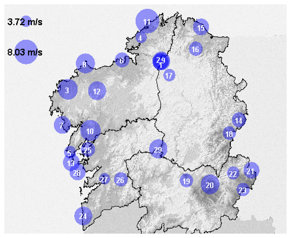
The analyzed region in this paper is Galicia, a region in northwest Spain, which is located in one of the windiest areas of Europe [27]. The Galician Meteorological Service, Meteogalicia, which is an entity that depends on the local government, publishes data from all the weather stations distributed around Galicia on its web page [28]. The data from these stations were used in this paper; however, only the windiest sites were selected to be studied. Wind speed data from the weather station in the Sotavento Experimental Wind Park [29,30], with measurements taken at heights of 20 m and 40 m, are also included in this paper. The 29 wind sites that were selected are listed in Table 1 and shown in Figure 1.
3. Wind Speed Distributions
Wind speed is typically measured at weather stations at a height of 10 m every 10 m. The resulting wind speed series can be represented as:
The basic representation of wind speed data is the histogram. The most common form of the histogram is obtained by splitting the range of data into equally sized bins, called classes. Each class is represented by the middle value of the bin. Therefore, each bin bj with Δν width has associated a relative frequency:
Finally, the chosen bin width Δν for the histogram can affect the fitting results [19,26]. However, the typical values used for wind energy analysis are 0.5 m/s or 1 m/s [13,19,26]. In this paper, following the international standards, the value of Δν = 0.5 m/s was selected.
The most widely used PDF to fit wind data is the Weibull distribution, which is defined as [2,21]:
4. Performance of Wind Energy Conversion Systems
The available power of the wind that crosses the rotor of a WTG is [9,31]:
When evaluating the available energy at a wind site, the following function is used:
This function is called the wind power density distribution and represents the distribution of wind energy at different wind speeds per unit of time and rotor area (W/m2). For a specific wind site, it can be obtained from Equation (5):
Therefore, the total wind power density Ew is:
When a Weibull PDF is considered, the following equation can be used [31]:
5. Energy Evaluation by Means of Power Curves
5.1. Power Curves
The energy production of a WTG can be obtained by means of its power curve, where the relationship between the wind speed and the delivered power is established, and can be expressed by the following (see Figure 2) [32]:
Several expressions can be used to represent the non-linear part of the power curve q(ν) [12,33,34]; however, for the sake of simplicity, the cubic equation is typically used [32,35–37]:
5.2. Energy Evaluation
To evaluate the energy production, the distribution of the energy generated by a WTG at different wind speeds per unit of time and rotor area is considered, which is called the power density distribution e(ν) in W/m2 and is defined as:
Taking into account Equation (11), the following equation can be used:
The total power density E at a specific wind site and WTG can be obtained from:
As a particular case, the power density E can be obtained analytically when the wind is represented by a Weibull PDF, and the WTG is modeled using a cubic power curve, see Equations (11) and (12). In this case, the following equation can be used [36,37]:
5.3. Weibull Parameters and Energy
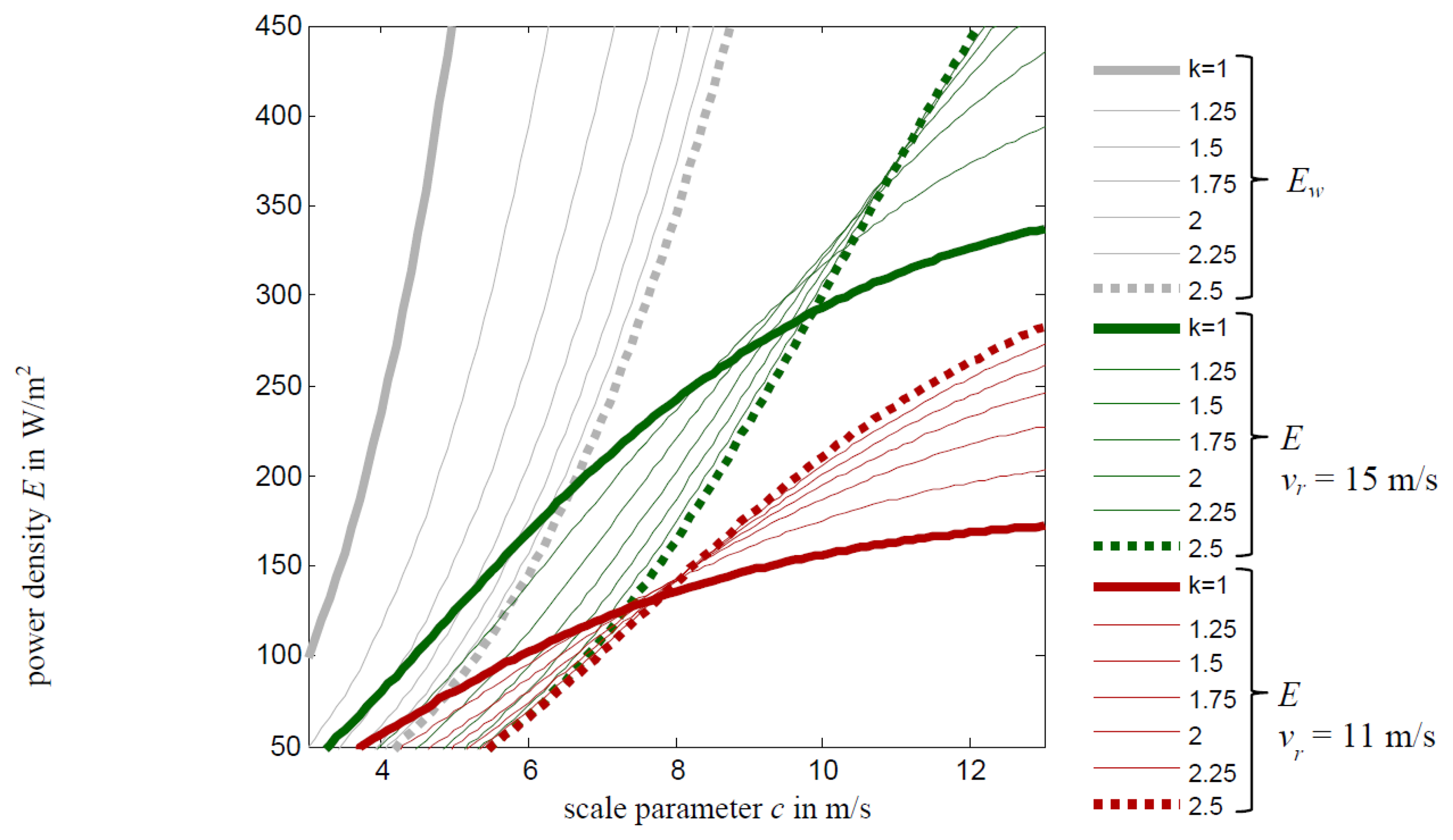
The impact of Weibull parameters, k and c, on the energy production can be analyzed using Equation (16). With this purpose, a set of wind power density Ew and power density E curves are shown in Figure 3, which were calculated using different scale and shape parameters (c and k). As shown in this figure, the relationship between the wind power density Ew with respect to the Weibull parameters, c and k, is clear: higher Ew values were obtained as c increased or k decreased. However, this statement is untrue when power density E is analyzed because for certain c and k values, the trend behavior is inverted.
In conclusion, the power density uncertainty cannot be associated with any variation interval of k and c values. Therefore, the fitting methods must be analyzed separately due to the error related to their use, as shown in the following sections.
5.4. Power Curve Parameters
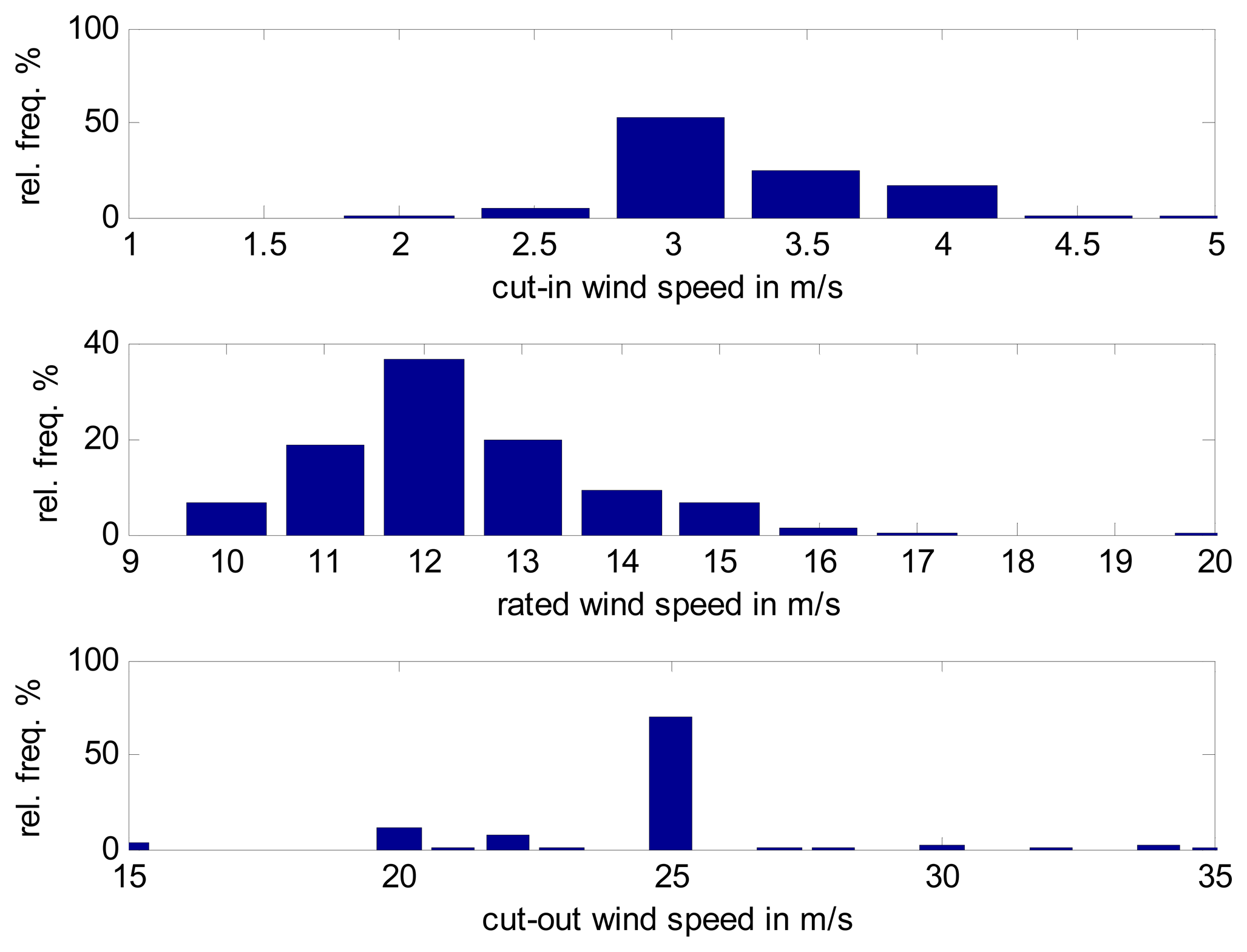
To characterize wind power curves, a database with WTG parameters [32] was used to obtain the relative frequencies and therefore, also obtain the distribution of the cut-in, cut-out and rated wind speeds, as shown in Figure 4. These values were used to define the cubic part of the power curve. After this analysis, the typical values for the cut-in wind speed (2.5–4.5 m/s), cut-out wind (20–35 m/s, typically 25 m/s) and rated wind speed (10–17 m/s) were obtained.
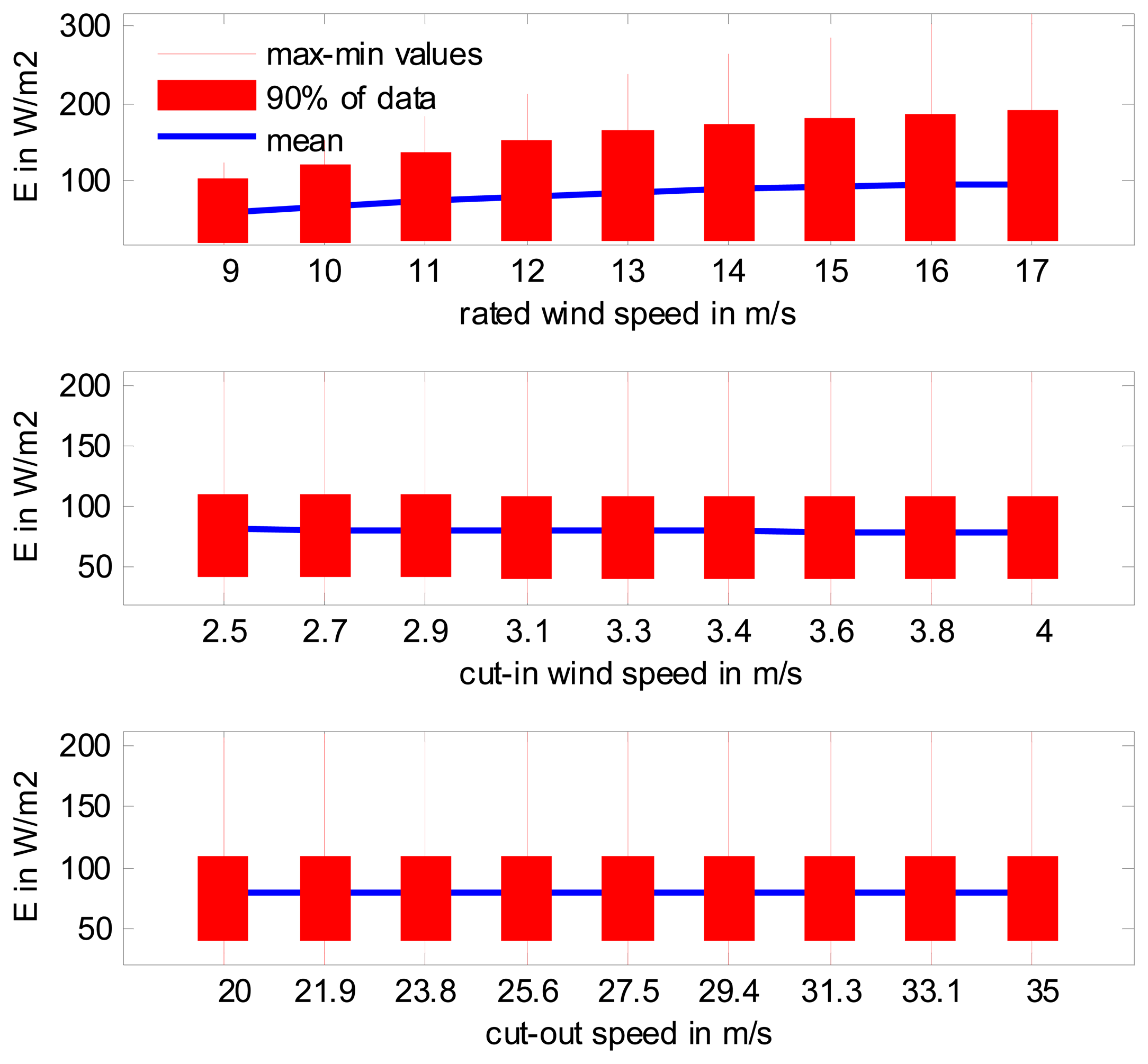
The rated wind speed has a greater effect than the cut-in wind speed or cut-out wind speed from the point of view of energy production [25,34,38], which can be verified with Figure 5, where a value of the power density E was calculated using the data from the wind sites discussed in Section 2. To obtain this figure, the values of the rated, cut-in and cut-out wind speeds were changed independently to study the individual effect of each parameter on the energy production values. The values presented in this section will be used to define the power curve expression used in the following sections.
6. Estimation Methods and Goodness of Fit
6.1. Estimation Methods
There are several ways to estimate a Weibull PDF to fit a wind speed distribution. The most widely used methods to calculate the Weibull parameters are the following (see Appendix A):
least square method (LSQM) or the graphical method [19,22,24,25,34,39];
maximum likelihood estimation (MLE) and modified maximum likelihood estimation (MMLE) [6,19,20,22,24–26,34];
In all the methods used in this paper, the lower wind speeds (calms) were treated separately [2,6] to improve the estimation results. Calm wind speeds were removed from the measurements; the fitting method was then applied to the remaining data. Finally, the calms speeds were re-introduced into the results to properly calculate the energy yield and other parameters.
6.2. Goodness of Fit
To determine if a theoretical PDF is suitable to describe the wind speed data, several indicators can be used. For each wind site and fitting method, the following indicators were considered:
The relative mean wind speed error (errorνm) and the mean wind speed data (νm) are compared with the resulting mean wind speed ( ) from the fitted PDF using:
The relative error of the available power density (errorEw):
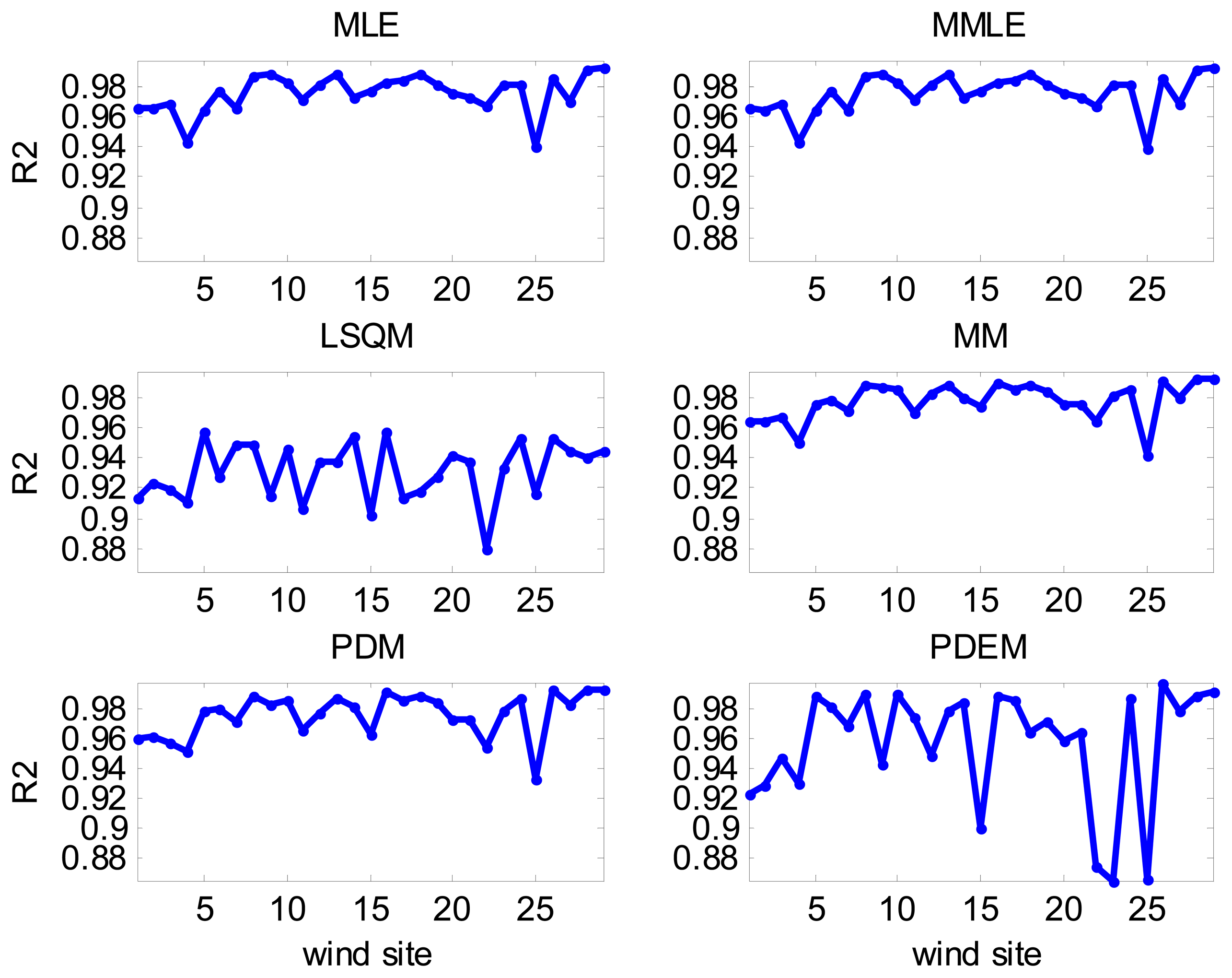
where Ew is calculated from the measured data; and is calculated from the estimated PDF.The coefficient of determination of the wind speed distribution (R2):
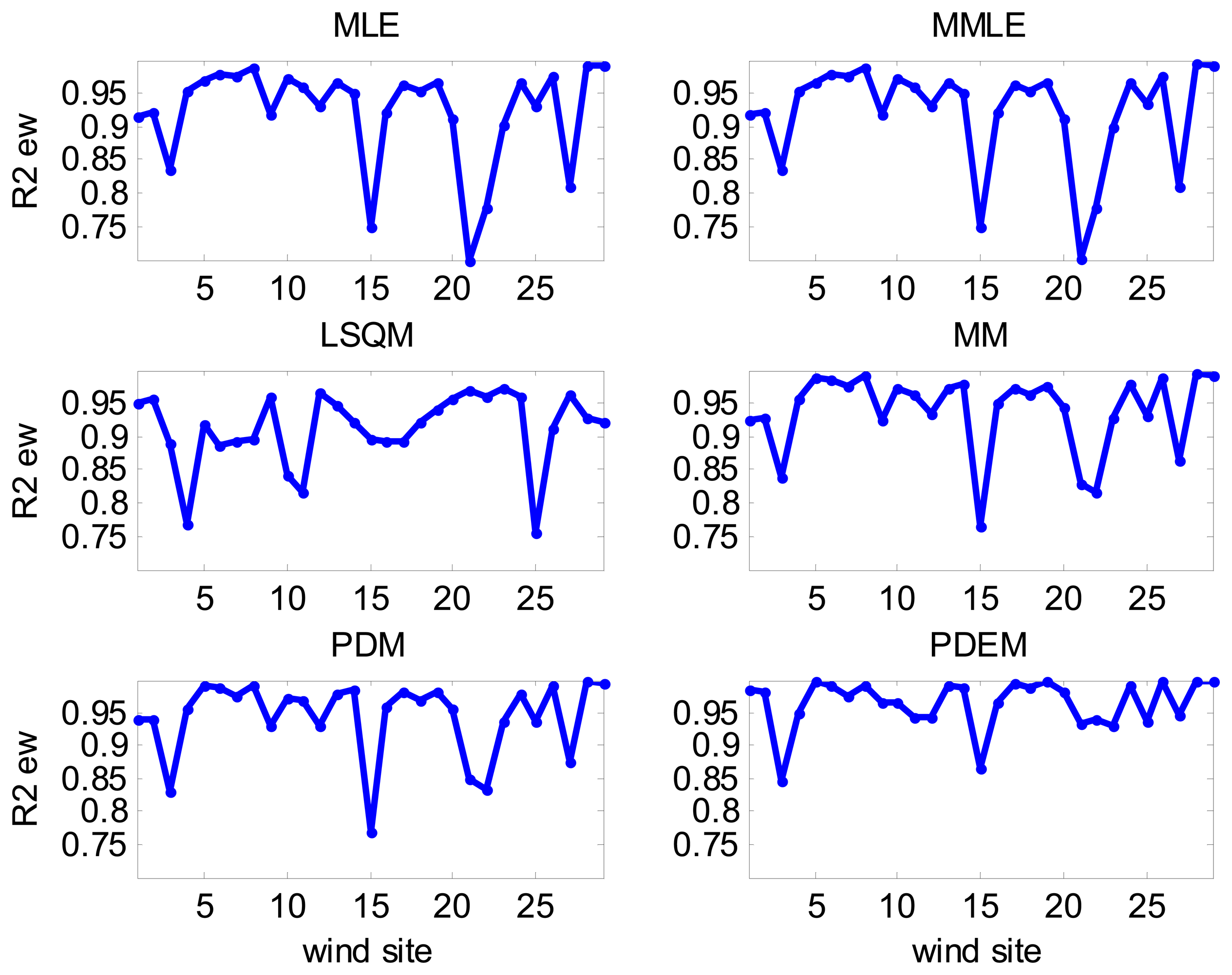
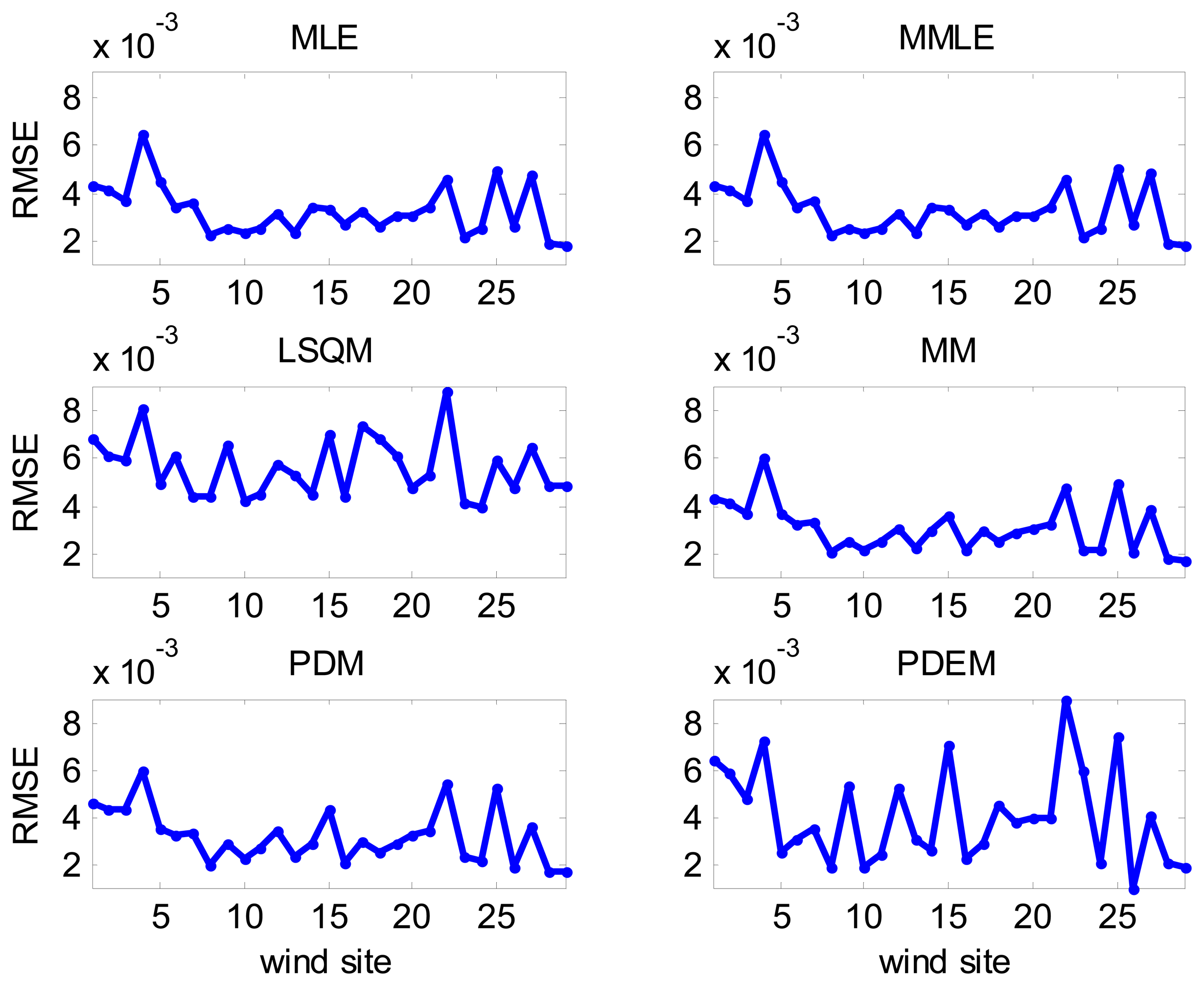
where is the estimated relative frequency of bin “j”; and is the mean of the frj values. In this case, the goodness of fit is better when the coefficient approaches 1. When R2 is applied to the distribution of the wind power density, the following indicator is obtained:where ēw is the mean of the ew(νj) values.Root mean square error (RMSE):
The goodness of fit is better when the RMSE approaches zero.
Goodness of fit parameters related to hypothesis testing methods, such as the Chi-square or Anderson-Darling methods, were not used in this work because their values strongly depend on the number of data points, which makes it difficult to compare results from different wind sites.
7. Estimation Method and Indicators of Fitness Based on WTG Energy Production
7.1. Proposed Indicators of Fitness
The energy produced by WTGs should be taken into account when Weibull PDFs are used in wind energy applications. For this reason, a set of indicators are proposed in the following paragraphs to include the energy output of WTGs in indicator calculations, which is done to increase the independence of the results from those obtained supposing a particular WTG or a reduced set [20,25,26].
For the aforementioned purpose, a set of power curves is considered, which is defined by selecting different rated wind speeds using Equation (14). In this case, the rated wind speeds νr is defined between 10 m/s and 17 m/s, according to the values shown in Section 5.4 (see Figure 4) and can be represented as:
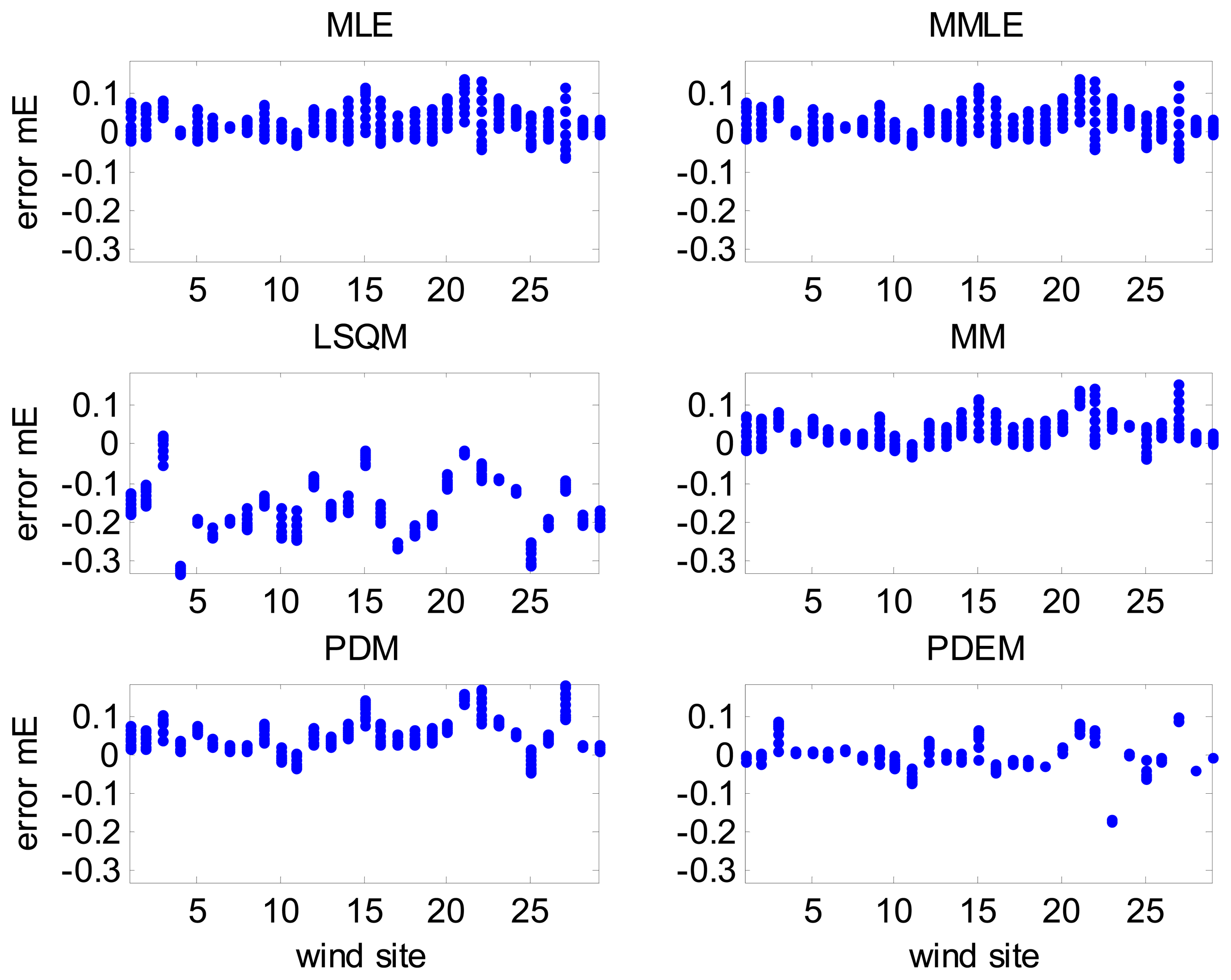
Relative error of power density (errormE), which is obtained as the mean value of power density errors at different rated wind speeds using the wind speed data and fitted PDF:
where El and are the total power density values calculated at a specific wind site using the wind speed data and the estimated PDF with the rated wind speed νrl, respectively.Coefficient of determination of the power density distribution , which is obtained as the mean value of the R2 values calculated with the power density distribution at different rated wind speeds using the wind speed data and fitted PDF:
where el and are the power density distributions calculated at a specific wind site using the data and the estimated PDF with the rated wind speed νrl, respectively, and e̅l is the mean for the el(νj) values.
7.2. Proposed Estimation Method: Part Density Energy Method (PDEM)
Regarding the methods to estimate the Weibull parameters, despite the fact that the estimation of energy produced by WTGs is one of the primary objectives in evaluating wind sites, the only method that partially takes it into account is the power density method (PDM), which uses the available energy associated with a wind speed distribution. In this context, the method, named the PDEM, which considers the typical behavior of power curves, is proposed in this paper, which is accomplished using a method that minimizes the following index:
The selection of νs in Equation (25) was done using the results shown in Figure 6. In this figure, the mean value and the STD of the values of errormE obtained from the PDEM method at all wind sites are represented against different νs values. As can be seen, at the selected νs, the mean error is at its minimum value. Therefore, a value of νs equal to 12 m/s was selected.
8. Parameter Estimation Results
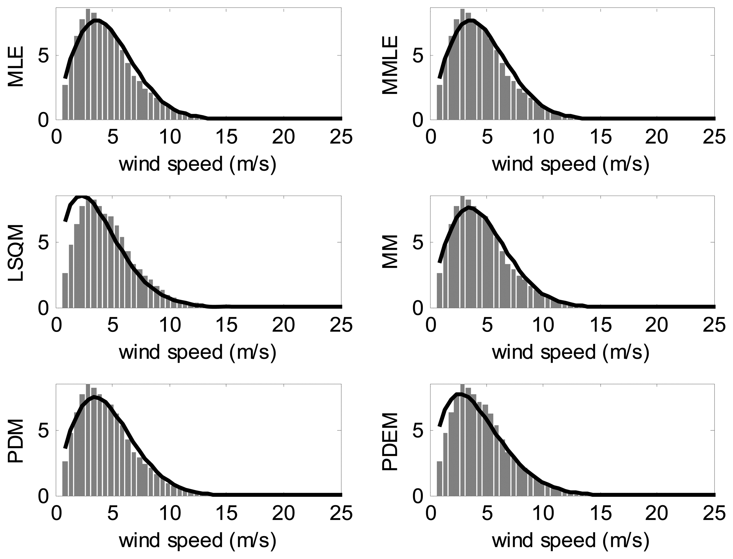
After choosing all the estimation methods (MLE, MMLE, LSQM, MM, PDM and PDEM), the methods were used to estimate the Weibull PDF parameters for each wind site. An example of the estimated PDF and distribution of the wind power density is plotted in Figures 7 and 8.
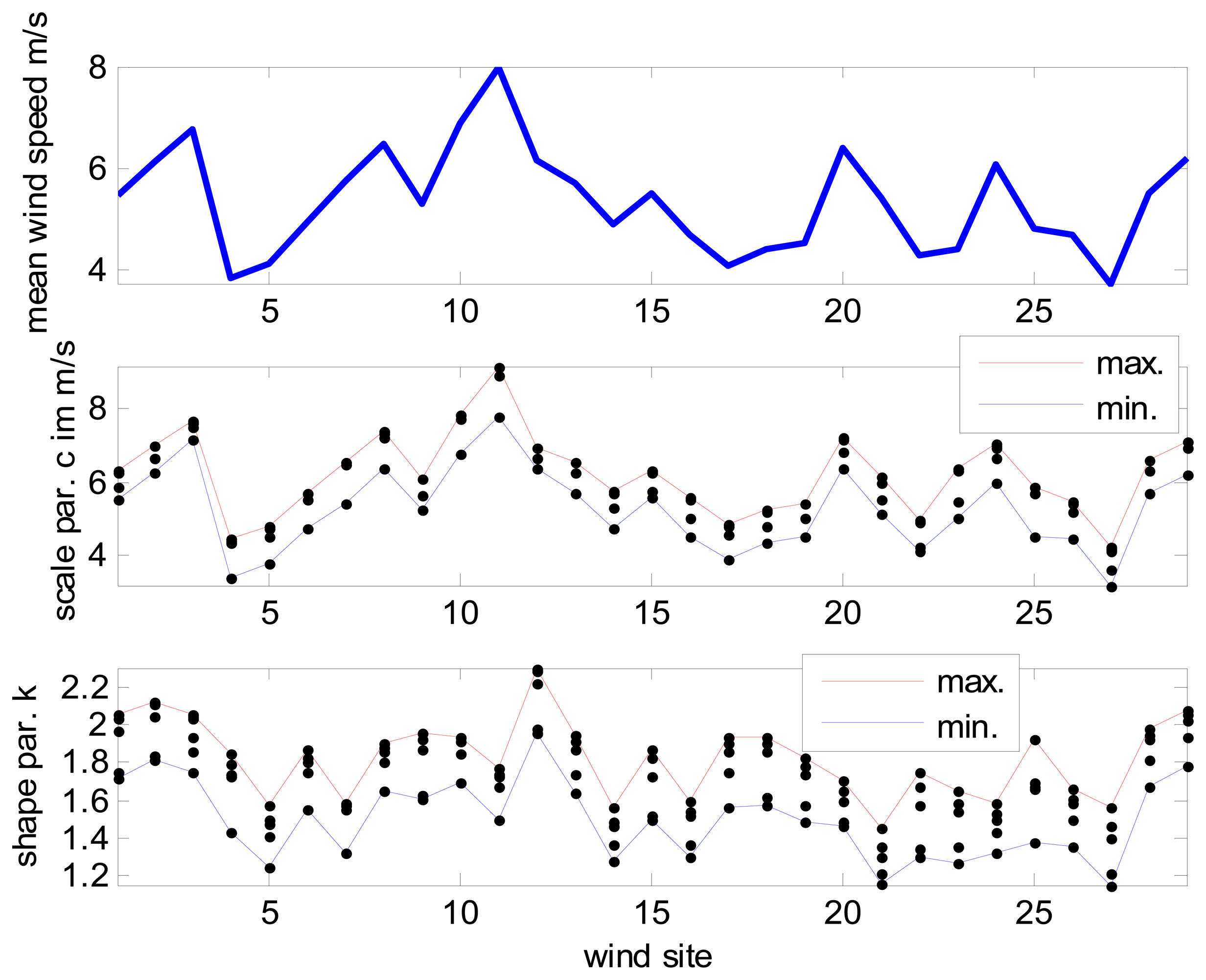
The Weibull parameters obtained for each wind site using the different fitting methods are shown in Table 2 and in Figure 9.
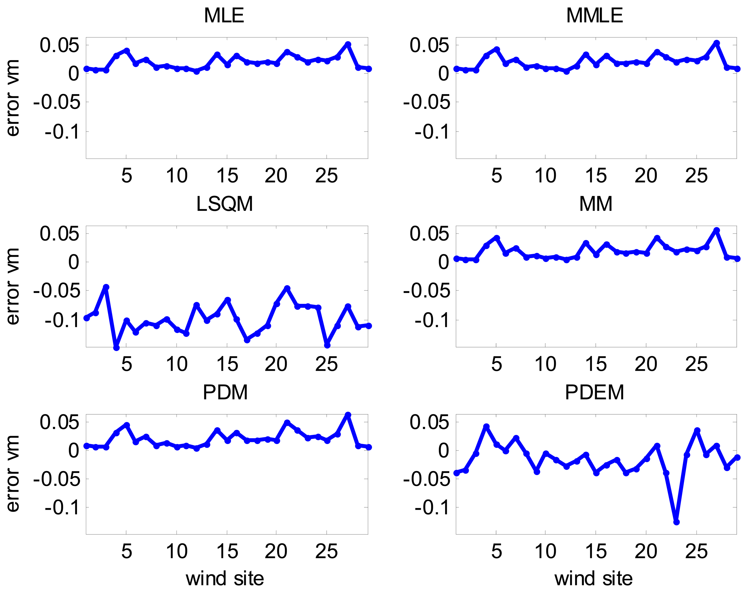
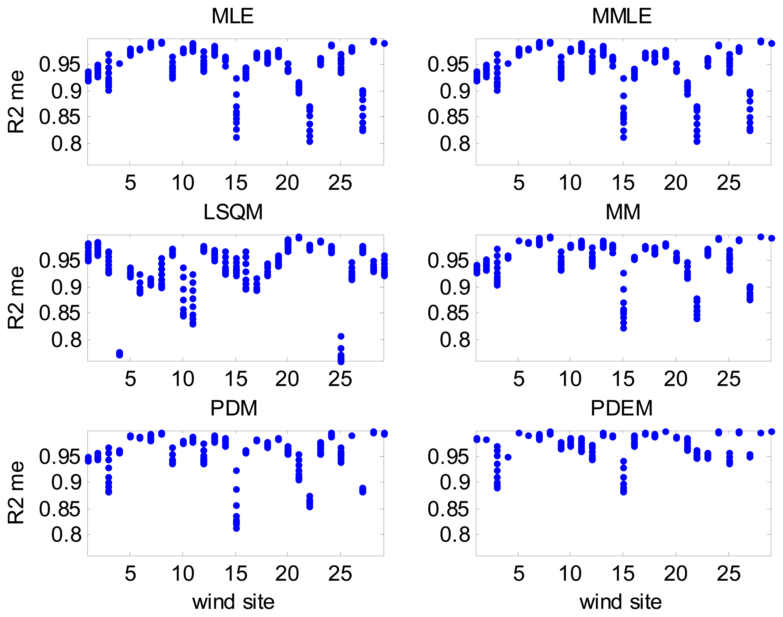
Once the parameters of the Weibull distribution are obtained, the goodness of fit indicators is calculated. The results for each wind site are displayed in Figures 10, 11, 12, 13, 14. 15 and 16. A summary of the results is presented in Table 3, which lists the mean and standard deviation (STD) of the indicator of the fitness values obtained for all wind sites for each estimation method.
To evaluate the fitting methods, all the fitness indicators should be taken into account because, for example, higher R2 values, when fitting wind, wind energy or energy, do not imply lower wind, wind energy or energy errors [26].
The following are the main conclusions regarding the fitting methods:
The proposed PDEM method exhibited the best behavior when the R2 values for wind power density and power density distributions were considered. In addition, this method has an acceptable behavior when the relative error of the wind power density and power density were taken into account. The overall behavior of the proposed method is extremely satisfactory.
MM exhibited the best behavior in wind distribution fitting according to the R2 and RMSE values [19]. Furthermore, the method resulted in acceptable values for all the indicators considered in this paper.
PDM's behavior is satisfactory with respect to estimating the mean wind speed; however, the method failed when the wind power production was considered [19,24].
LSQM, in terms of relative error, strongly depended on the wind site data, as can be seen in the high values shown by the STD of its errors (errorνm, errorEw and errormE) [19,20,22].
In conclusion, the proposed PDEM is the most suitable method when the focus of the analysis is on the energy produced by WTGs. Nevertheless, other methods, particularly MM, exhibited satisfactory results in terms of energy fitness.
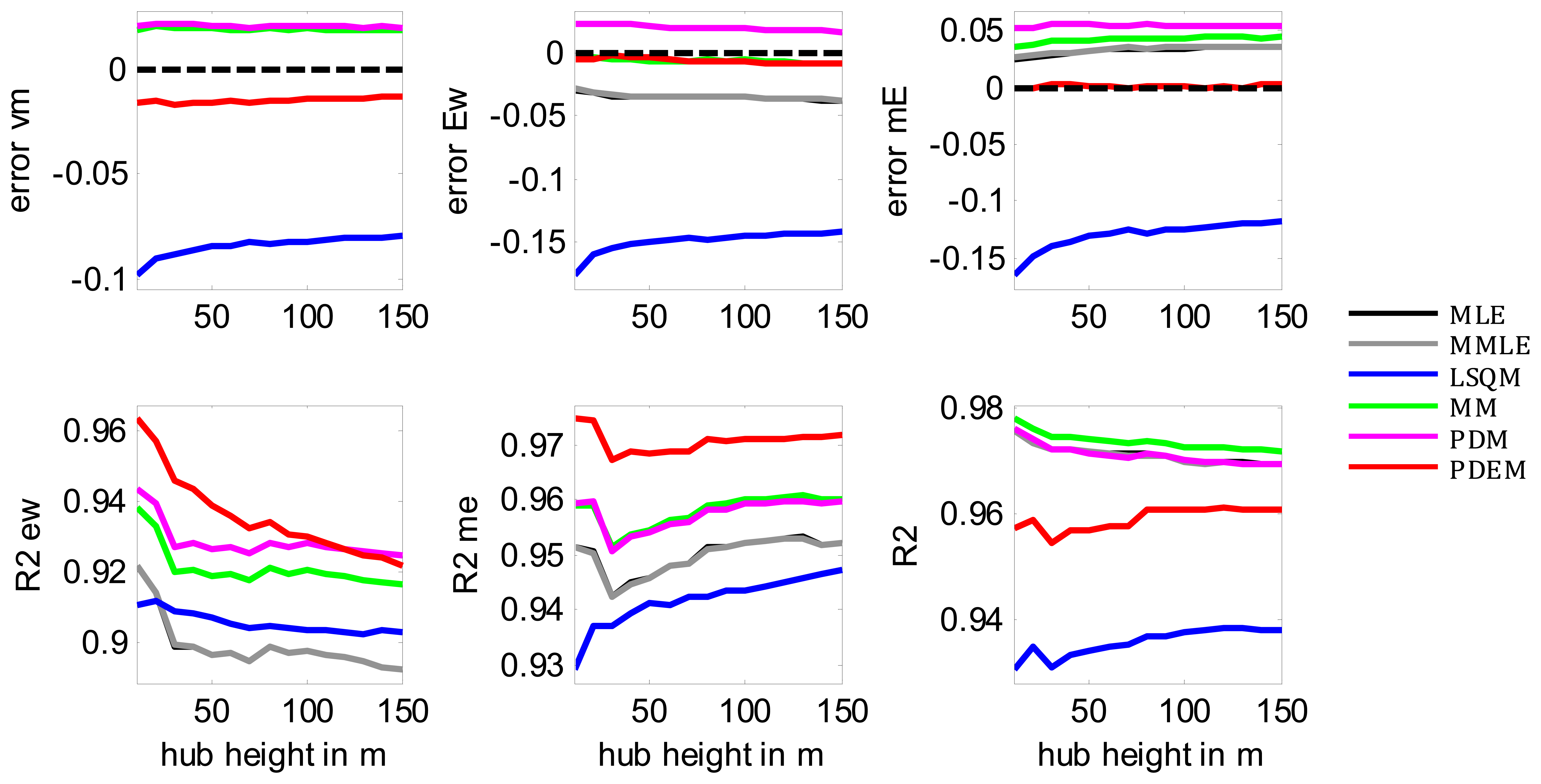
To evaluate the robustness of the proposed PDEM, the behaviour of the different fitting methods with an estimated wind speed at different hub heights is shown in Appendix B, where it can be seen that similar conclusions are achieved.
9. Conclusions
This paper presents an analysis of wind speed data based on using fitting curve methods to obtain the parameters of the Weibull PDF. The most widely used methods were selected for this analysis. Furthermore, a method, called PDEM, which takes into account the power density distribution and the typical performance of WTGs, is presented.
The results of the fitting methods in obtaining the Weibull parameters were evaluated by a set of indicators defined from wind speeds and wind power density distributions. Additionally, the indicators, errormE and , which consider the behavior of WTGs in terms of energy production, are introduced.
As the primary conclusion, the proposed PDEM method exhibited the best results when the energy produced by the WTGs is considered. Furthermore, its result when all indicators are taken into account, are extremely satisfactory. Nevertheless, other methods, particularly MM, exhibited satisfactory results in terms of energy fitness. In this paper, wind speed data from weather stations from a specific region, northwest Spain (Galicia), were used.
Acknowledgments
The authors would like to thank the personnel at Sotavento Experimental Wind Park for their contribution and help with field experience and for their accessibility to the measurement data. This work was supported in part by the Consellería of Innovación e Industria xunta de Galicia, Spain) under contract 07REM008V19PR and the Ministry of Science and Innovation (Spain; under contracts ENE 2007-67473 and ENE 2009-13074.
Conflicts of Interest
The authors declare no conflict of interest.
Appendix
A. Fitting Methods of the Weibull Parameters
In the following paragraphs, the most common methods to obtain the scale and form parameters for a Weibull PDF are described.
A1. MLE
The Weibull parameters are those that maximize their joint probability of occurrence and can be obtained by solving the following:
Using data from a histogram, the modified maximum likelihood method (MMLM) results [20] in the following:
A2. LSQM
The LSQM, also known as the Weibull plot, is based on logarithmic transformations applied to the Weibull cumulative distribution function F(ν) and thus, can be represented by a straight line:
The Weibull parameters can be obtained from:
Finally, the line parameters are obtained from:
The LSQM is extremely popular due to its simplicity; however, the logarithmic transformations used during the calculation tend to cause some inaccuracy [20].
A3. MM
The MM is based on obtaining the Weibull parameters using certain statistical moments calculated using wind speed data. When the mean wind speed (νm) and the STD (σ) of wind data are used, the following relationship can be obtained [24]:
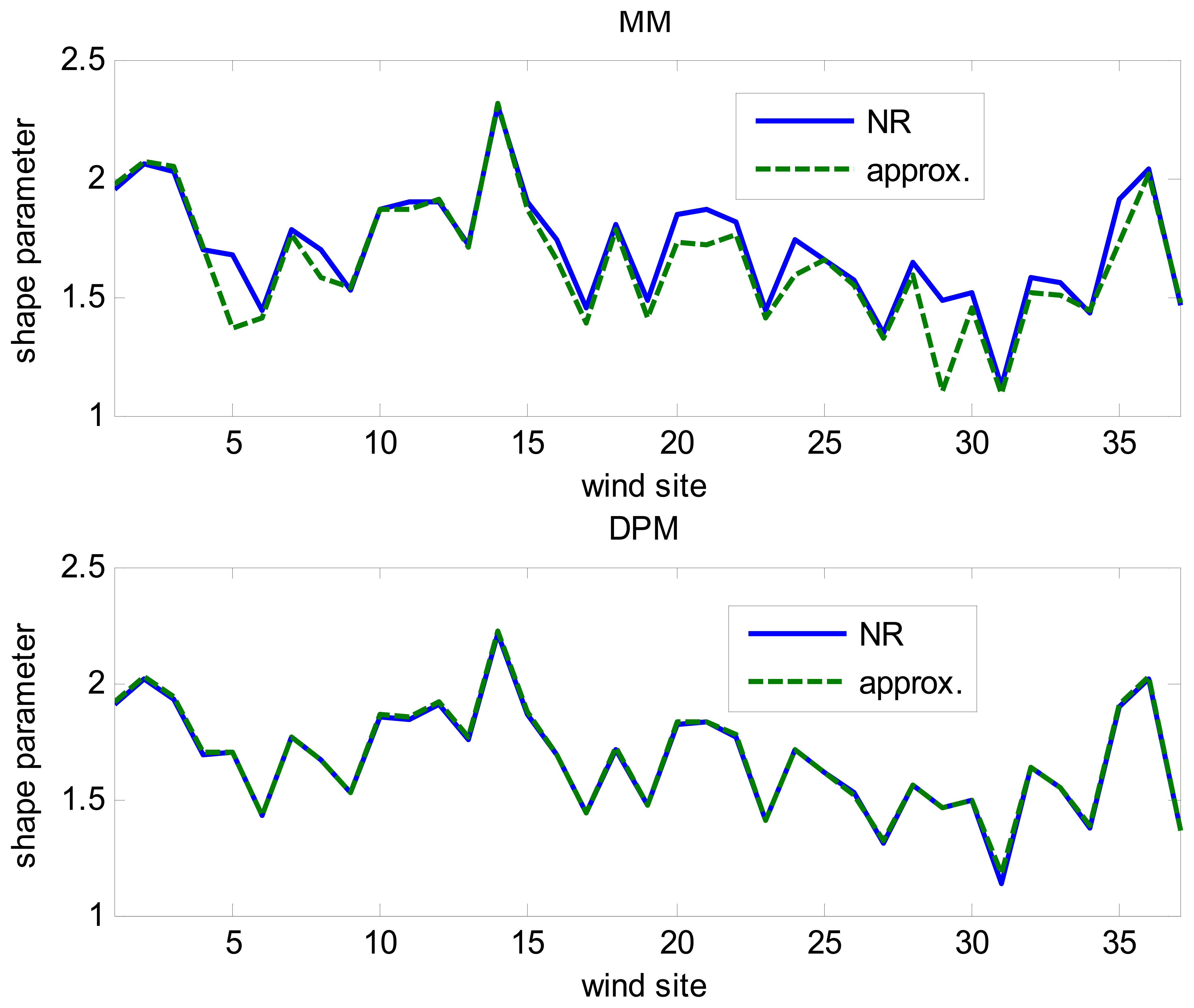
The shape parameter k can be calculated from this equation by the Newton-Raphson (NR) method:
The comparison between the approximate solution using Equation (A10) and the solution solving Equation (A9) by the Newton Raphson method is shown in Figure 17. To avoid errors, the approximated solution was not used in this paper.
A4. PDM
The PDM uses the Energy Pattern Factor [24,25]:
This factor relates to the shape parameter k by means of:
Using the NR method to solve this equation, the following expressions are obtained:
The following approximated expression can be used, which assumes that Epf is typically between 1.45 and 4.4:
Both results from using Equations (A13) and (A14) are shown in Figure 17. To avoid errors, the approximated solution was not used in this paper.
B. Behavior of the Proposed PDEM Method at Different Hub Heights
In order to evaluate the robustness of the proposed PDEM method, it has been evaluated using wind speeds at different hub heights. For this purpose, wind speeds have been estimated using a logaritmic wind profile with a roughness length of 0.05 m, which is a common value in wind farms [9,12]. The resulting mean values of the indicators of the fitness (errorνm, errorEw, errormE, R2ew, R2me and R2) for heights between 10 m and 150 m can be seen in Figure 18. As a conclusion, the overall relative behaviour of the proposed PDEM method does not significantly change with the hub height.
References
- Global Wind Energy Council (GWEC). Global statistics. Available online: http://www.gwec.net/global-figures/graphs/ (accessed on 15 March 2014).
- Tuller, S.; Brett, A. The characteristics of wind velocity that favor the fitting of a Weibull distribution in wind speed analysis. J. Appl. Meteorol. 1984, 23, 124–134. [Google Scholar]
- Carrillo, C.; Feijóo, A.E. Power fluctuations in an isolated wind plant. IEEE Trans. Energy Convers. 2004, 19, 217–221. [Google Scholar]
- Cidrás, J.; Carrillo, C.; Feijóo, A.E. Probabilistic model for mechanical power fluctuations in asynchronous wind parks. IEEE Trans. Power Syst. 2003, 18, 761–768. [Google Scholar]
- Carrillo, C.; Díaz-Dorado, E. PSCAD/EMTDC-Based Modeling and Flicker Estimation for Wind Turbines. Proceedings of the European Wind energy Conference (EWEC '09), Marseille, France, 16–19 March 2009; Volume 9, pp. 3091–3127.
- Carta, J.A.; Ramírez, P.; Velázquez, S. A review of wind speed probability distributions used in wind energy analysis. Renew. Sustain. Energy Rev. 2009, 13, 933–955. [Google Scholar]
- Usta, I.; Kantar, Y.M. Analysis of some flexible families of distributions for estimation of wind speed distributions. Appl. Energy 2012, 89, 355–367. [Google Scholar]
- Celik, A.N.; Makkawi, A.; Muneer, T. Critical evaluation of wind speed frequency distribution functions. J. Renew. Sustain. Energy 2010, 2. [Google Scholar] [CrossRef]
- Burton, T.; Sharpe, D.; Jenkins, N.; Bossanyi, E. Wind Energy Handbook; John Wiley & Sons, Ltd.: Chichester, UK, 2001. [Google Scholar]
- WAsP—The Wind Atlas Analysis and Application Program. Available online: http://www.wasp.dk (accessed on 15 March 2014).
- Instituto para la Diversificación y Ahorro de la Energía (IDEA). Atlas Eólico de España. Available online: http://atlaseolico.idae.es (accessed on 15 March 2014). In Sapinish.
- Justus, C.G. Nationwide assessment of potential output from wind-powered generators. J. Appl. Meteorol. 1976, 15, 673–678. [Google Scholar]
- Wind Turbines—Part. 12-1: Power Performance Measurements of Electricity Producing Wind Turbines; IEC 61400-12-1 Edition 1.0; International Electrotechnical Commission (IEC): Geneva, Switzerland, 2005.
- Feijóo, A.E.; Cidrás, J.; García-Dornelas, J.L. Wind speed simulation in wind farms for steady-state security assessment of electrical power systems. IEEE Trans. Energy Convers. 1999, 14, 1582–1588. [Google Scholar]
- Feijóo, A.E.; Carrillo, C.; Cidrás, J. Modelos de Generadores Asíncronos Para la Evaluación de Perturbaciones Emitidas Por Parques Eólicos. Proceedings of the X Reunión de Grupos de Investigación en Ingeniería Eléctrica, Santander, Spain, 18 March 2000; pp. 1–5, In Spanish.
- Huang, S.J.; Wan, H. Enhancement of matching turbine generators with wind regime using capacity factor curves strategy. IEEE Trans. Energy Convers. 2009, 24, 551–553. [Google Scholar]
- Hu, S.; Cheng, J. Performance evaluation of pairing between sites and wind turbines. Renew. Energy 2007, 32, 1934–1947. [Google Scholar]
- Celik, A.N. Assessing the suitability of wind speed probabilty distribution functions based on wind power density. Renew. Energy 2003, 28, 1563–1574. [Google Scholar]
- Chang, T.P. Performance comparison of six numerical methods in estimating Weibull parameters for wind energy application. Appl. Energy 2011, 88, 272–282. [Google Scholar]
- Seguro, J.V.; Lambert, T.W. Modern estimation of the parameters of the Weibull wind speed distribution for wind energy analysis. J. Wind Eng. Ind. Aerodyn. 2000, 85, 75–84. [Google Scholar]
- Edwards, P.J.; Hurst, R.B. Level-crossing statistics of the horizontal wind speed in the planetary surface boundary layer. Chaos 2001, 11, 611–618. [Google Scholar]
- Costa Rocha, P.A.; de Sousa, R.C.; de Andrade, C.F.; da Silva, M.E.V. Comparison of seven numerical methods for determining Weibull parameters for wind energy generation in the northeast region of Brazil. Appl. Energy 2012, 89, 395–400. [Google Scholar]
- García-Bustamante, E.; González-Rouco, J.F.; Jiménez, P.A.; Navarro, J.; Montávez, J.P. The influence of the Weibull assumption in monthly wind energy estimation. Wind Energy 2008, 11, 483–502. [Google Scholar]
- Akdağ, S.A.; Dinler, A. A new method to estimate Weibull parameters for wind energy applications. Energy Convers. Manag. 2009, 50, 1761–1766. [Google Scholar]
- Stevens, M.; Smulders, P. The estimation of the parameters of the Weibull wind speed distribution for wind energy utilization purposes. Wind Eng. 1979, 3, 132–145. [Google Scholar]
- Carta, J.A.; Ramírez, P.; Velázquez, S. Influence of the level of fit of a density probability function to wind-speed data on the WECS mean power output estimation. Energy Convers. Manag. 2008, 49, 2647–2655. [Google Scholar]
- Troen, I.; Petersen, E.L. European Wind Atlas; Riso National Laboratory: Roskilde, Denmark, 1989; p. 656. [Google Scholar]
- Penabad, E.; Álvarez, I.; Balseiro, C.F.; DeCastro, M.; Gómez, B.; Pérez-Muñuzuri, V.; Gómez-Gesteira, M. Comparative analysis between operational weather prediction models and QuikSCAT wind data near the Galician coast. J. Mar. Syst. 2008, 72, 256–270. [Google Scholar]
- López, J.; Dorado, A.; Álvarez, J. The Sotavento Experimental Wind Park. Proceedings of the Global Windpower Conference, Paris, France, 2–5 April 2002; pp. 36–38.
- Díaz-Dorado, E.; Carrillo, C.; Cidrás, J. Control algorithm for coordinated reactive power compensation in a wind park. IEEE Trans. Energy Convers. 2008, 23, 1064–1072. [Google Scholar]
- Johnson, G.L. Wind Energy Systems; Kansas State University: Manhattan, KS, USA, 2006; p. 449. [Google Scholar]
- Carrillo, C.; Obando Montaño, A.F.; Cidrás, J.; Díaz-Dorado, E. Review of power curve modelling for wind turbines. Renew. Sustain. Energy Rev. 2013, 21, 572–581. [Google Scholar]
- Giorsetto, P.; Utsurogi, K. Development of a new procedure for reliability modeling of wind turbine generators. IEEE Trans. Power Appar. Syst. 1983, PAS-102, 134–143. [Google Scholar]
- Mathew, S. Wind Energy: Fundamentals, Resource Analysis and Economics; Springer: Berlin/Heidelberg, Germany, 2006; p. 252. [Google Scholar]
- Thiringer, T.; Linders, J. Control by variable rotor speed of a fixed-pitch wind turbine operating in a wide speed range. IEEE Trans. Energy Convers. 1993, 8, 520–526. [Google Scholar]
- Jangamshetti, S.H.; Rau, V.G. Normalized power curves as a tool for identification of optimum wind turbine generator parameters. IEEE Trans. Energy Convers. 2001, 16, 283–288. [Google Scholar]
- Albadi, M.H.; El-Saadany, E.F. Wind turbines capacity factor modeling—A novel approach. IEEE Trans. Power Syst. 2009, 24, 1637–1638. [Google Scholar]
- Mathew, S.; Pandey, K.P.; Kumar, V.A. Analysis of wind regimes for energy estimation. Renew. Energy 2002, 25, 381–399. [Google Scholar]
- Jamil, M.; Parsa, S.; Majidi, M. Wind power statistics and an evaluation of wind energy density. Renew. Energy 1995, 6, 623–628. [Google Scholar]
- Lagarias, J.C.; Reeds, J.A.; Wright, M.H.; Wright, P.E. Convergence properties of the Nelder-Mead simplex method in low dimensions. SIAM J. Optim. 1998, 9, 112–147. [Google Scholar]


| No. | Name | MWS | ND | No. | Name | MWS | ND |
|---|---|---|---|---|---|---|---|
| 1 | P.E. Sotavento 20 m | 5.5 | 6.6 | 16 | LU Fragavella | 4.7 | 4.1 |
| 2 | P.E. Sotavento 40 m | 6.1 | 6.6 | 17 | LU Guitiriz | 4.1 | 9.7 |
| 3 | CO A Gandara | 6.8 | 1.1 | 18 | LU O Cebreiro | 4.4 | 1.1 |
| 4 | CO Aldea Nova | 3.8 | 1.3 | 19 | OU Alto de Rodicio | 4.5 | 5.6 |
| 5 | CO Corrubedo | 4.1 | 9.1 | 20 | OU Cabeza de Manzaneda | 6.4 | 3.2 |
| 6 | CO Corunha Dique | 4.9 | 2.8 | 21 | OU Lardeira | 5.4 | 3.0 |
| 7 | CO Lira | 5.8 | 0.4 | 22 | OU Serra do Eixe | 4.3 | 2.4 |
| 8 | CO Malpica | 6.5 | 4.6 | 23 | OU Xares | 4.4 | 2.9 |
| 9 | CO Marco da Curra | 5.3 | 6.4 | 24 | PO Castro Vicaludo | 6.1 | 6.3 |
| 10 | CO Muralla | 6.9 | 3.8 | 25 | PO Coron | 4.8 | 8.1 |
| 11 | CO Punta Candieira | 8.0 | 4.4 | 26 | PO Fornelos de Montes | 4.7 | 7.1 |
| 12 | CO Rio do Sol | 6.1 | 1.5 | 27 | PO O Viso | 3.7 | 2.3 |
| 13 | CO Salvora | 5.7 | 4.0 | 28 | PO Ons | 5.5 | 5.1 |
| 14 | LU Ancares | 4.9 | 8.4 | 29 | PO Serra do Faro | 6.2 | 3.9 |
| 15 | LU Burela | 5.5 | 3.6 | - | - | - | - |
| WN | MLE | MMLE | LSQM | MM | PDM | PDEM | ||||||
|---|---|---|---|---|---|---|---|---|---|---|---|---|
| c | k | c | k | c | k | c | k | c | k | c | k | |
| 1 | 6.3 | 2.1 | 6.3 | 2.1 | 5.5 | 1.7 | 6.3 | 2.0 | 6.3 | 2.0 | 5.9 | 1.7 |
| 2 | 7.0 | 2.1 | 7.0 | 2.1 | 6.3 | 1.8 | 7.0 | 2.1 | 7.0 | 2.0 | 6.6 | 1.8 |
| 3 | 7.7 | 2.1 | 7.7 | 2.1 | 7.2 | 1.7 | 7.6 | 2.0 | 7.6 | 1.9 | 7.5 | 1.9 |
| 4 | 4.4 | 1.8 | 4.4 | 1.8 | 3.4 | 1.4 | 4.4 | 1.7 | 4.4 | 1.7 | 4.5 | 1.9 |
| 5 | 4.8 | 1.6 | 4.8 | 1.6 | 3.8 | 1.2 | 4.8 | 1.5 | 4.8 | 1.5 | 4.5 | 1.4 |
| 6 | 5.7 | 1.9 | 5.7 | 1.9 | 4.8 | 1.6 | 5.7 | 1.8 | 5.7 | 1.8 | 5.6 | 1.7 |
| 7 | 6.5 | 1.6 | 6.5 | 1.6 | 5.4 | 1.3 | 6.5 | 1.6 | 6.5 | 1.6 | 6.5 | 1.6 |
| 8 | 7.4 | 1.9 | 7.4 | 1.9 | 6.4 | 1.7 | 7.4 | 1.9 | 7.4 | 1.9 | 7.2 | 1.8 |
| 9 | 6.1 | 2.0 | 6.1 | 2.0 | 5.3 | 1.6 | 6.1 | 1.9 | 6.1 | 1.9 | 5.7 | 1.6 |
| 10 | 7.9 | 1.9 | 7.9 | 1.9 | 6.8 | 1.7 | 7.8 | 1.9 | 7.8 | 1.9 | 7.7 | 1.8 |
| 11 | 9.2 | 1.7 | 9.2 | 1.7 | 7.8 | 1.5 | 9.2 | 1.7 | 9.2 | 1.8 | 8.9 | 1.7 |
| 12 | 6.9 | 2.3 | 6.9 | 2.3 | 6.4 | 2.0 | 6.9 | 2.3 | 6.9 | 2.2 | 6.7 | 2.0 |
| 13 | 6.6 | 1.9 | 6.6 | 1.9 | 5.7 | 1.6 | 6.5 | 1.9 | 6.5 | 1.9 | 6.3 | 1.7 |
| 14 | 5.8 | 1.6 | 5.8 | 1.6 | 4.7 | 1.3 | 5.7 | 1.5 | 5.7 | 1.5 | 5.3 | 1.4 |
| 15 | 6.3 | 1.9 | 6.3 | 1.9 | 5.6 | 1.5 | 6.3 | 1.8 | 6.3 | 1.7 | 5.7 | 1.5 |
| 16 | 5.6 | 1.6 | 5.6 | 1.6 | 4.6 | 1.3 | 5.5 | 1.5 | 5.5 | 1.5 | 5.0 | 1.4 |
| 17 | 4.9 | 1.9 | 4.8 | 1.9 | 3.9 | 1.6 | 4.8 | 1.9 | 4.8 | 1.9 | 4.6 | 1.7 |
| 18 | 5.2 | 1.9 | 5.2 | 1.9 | 4.3 | 1.6 | 5.2 | 1.9 | 5.2 | 1.9 | 4.8 | 1.6 |
| 19 | 5.4 | 1.8 | 5.4 | 1.8 | 4.5 | 1.5 | 5.4 | 1.8 | 5.4 | 1.7 | 5.0 | 1.6 |
| 20 | 7.2 | 1.7 | 7.2 | 1.7 | 6.4 | 1.5 | 7.2 | 1.6 | 7.2 | 1.6 | 6.8 | 1.5 |
| 21 | 6.1 | 1.5 | 6.1 | 1.5 | 5.1 | 1.2 | 6.0 | 1.3 | 6.0 | 1.3 | 5.6 | 1.2 |
| 22 | 5.0 | 1.8 | 5.0 | 1.8 | 4.1 | 1.3 | 4.9 | 1.7 | 4.9 | 1.6 | 4.3 | 1.3 |
| 23 | 6.4 | 1.7 | 6.4 | 1.7 | 5.5 | 1.4 | 6.3 | 1.6 | 6.3 | 1.5 | 5.0 | 1.3 |
| 24 | 7.0 | 1.6 | 7.0 | 1.6 | 6.0 | 1.3 | 7.0 | 1.5 | 7.0 | 1.5 | 6.7 | 1.4 |
| 25 | 5.7 | 1.7 | 5.7 | 1.7 | 4.5 | 1.4 | 5.7 | 1.7 | 5.7 | 1.7 | 5.9 | 1.9 |
| 26 | 5.5 | 1.7 | 5.5 | 1.7 | 4.5 | 1.3 | 5.5 | 1.6 | 5.5 | 1.6 | 5.2 | 1.5 |
| 27 | 4.2 | 1.6 | 4.2 | 1.6 | 3.2 | 1.1 | 4.2 | 1.5 | 4.2 | 1.4 | 3.7 | 1.2 |
| 28 | 6.6 | 2.0 | 6.6 | 2.0 | 5.7 | 1.7 | 6.6 | 2.0 | 6.6 | 1.9 | 6.3 | 1.8 |
| 29 | 7.1 | 2.1 | 7.1 | 2.1 | 6.2 | 1.8 | 7.1 | 2.1 | 7.1 | 2.0 | 6.9 | 1.9 |
| Fitness indicator | MLE | MMLE | LSQM | MM | PDM | PDEM | |
|---|---|---|---|---|---|---|---|
| errorνm | Mean | 2.0% | 2.0% | −9.7% | 1.9% | 2.1% | −1.6% |
| STD | 1.1% | 1.2% | 2.5% | 1.3% | 1.4% | 3.0% | |
| errorEw | Mean | −2.9% | −2.9% | −17.4% | −0.5% | 2.3% | −0.6% |
| STD | 3.8% | 3.8% | 5.7% | 2.5% | 1.5% | 4.2% | |
| errormE | Mean | 2.7% | 2.7% | −16.2% | 3.7% | 5.4% | −0.1% |
| STD | 2.5% | 2.5% | 7.7% | 2.9% | 4.1% | 4.9% | |
| R2 | Mean | 0.976 | 0.976 | 0.931 | 0.978 | 0.976 | 0.957 |
| STD | 0.012 | 0.013 | 0.019 | 0.012 | 0.014 | 0.038 | |
| R2ew | Mean | 0.922 | 0.922 | 0.911 | 0.938 | 0.944 | 0.964 |
| STD | 0.074 | 0.074 | 0.055 | 0.059 | 0.057 | 0.037 | |
| R2me | Mean | 0.952 | 0.952 | 0.930 | 0.959 | 0.959 | 0.975 |
| STD | 0.039 | 0.039 | 0.053 | 0.035 | 0.038 | 0.024 | |
| RMSE | Mean | 0.3% | 0.3% | 0.6% | 0.3% | 0.3% | 0.4% |
| STD | 0.1% | 0.1% | 0.1% | 0.1% | 0.1% | 0.2% | |
© 2014 by the authors; licensee MDPI, Basel, Switzerland. This article is an open access article distributed under the terms and conditions of the Creative Commons Attribution license( http://creativecommons.org/licenses/by/3.0/).
Share and Cite
Carrillo, C.; Cidrás, J.; Díaz-Dorado, E.; Obando-Montaño, A.F. An Approach to Determine the Weibull Parameters for Wind Energy Analysis: The Case of Galicia (Spain). Energies 2014, 7, 2676-2700. https://doi.org/10.3390/en7042676
Carrillo C, Cidrás J, Díaz-Dorado E, Obando-Montaño AF. An Approach to Determine the Weibull Parameters for Wind Energy Analysis: The Case of Galicia (Spain). Energies. 2014; 7(4):2676-2700. https://doi.org/10.3390/en7042676
Chicago/Turabian StyleCarrillo, Camilo, José Cidrás, Eloy Díaz-Dorado, and Andrés Felipe Obando-Montaño. 2014. "An Approach to Determine the Weibull Parameters for Wind Energy Analysis: The Case of Galicia (Spain)" Energies 7, no. 4: 2676-2700. https://doi.org/10.3390/en7042676
APA StyleCarrillo, C., Cidrás, J., Díaz-Dorado, E., & Obando-Montaño, A. F. (2014). An Approach to Determine the Weibull Parameters for Wind Energy Analysis: The Case of Galicia (Spain). Energies, 7(4), 2676-2700. https://doi.org/10.3390/en7042676