Localized Climate and Surface Energy Flux Alterations across an Urban Gradient in the Central U.S.

Abstract

Long-term urban and rural climate data spanning January 1995 through October 2013 were analyzed to investigate the Urban Heat Island (UHI) effect in a representative mid-sized city of the central US. Locally distributed climate data were also collected at nested low density urban, recently developed, and high density urban monitoring sites from June through September 2013 to improve mechanistic understanding of spatial variability of the UHI effect based upon urban land use intensity. Long-term analyses (1995–2013) indicate significant differences (p < 0.001) between average air temperature (13.47 and 12.89 °C, at the urban and rural site respectively), relative humidity (69.11% and 72.51%, urban and rural respectively), and average wind speed (2.05 and 3.15 m/s urban and rural respectively). Significant differences (p < 0.001) between urban monitoring sites indicate an urban microclimate gradient for all climate variables except precipitation. Results of analysis of net radiation and soil heat flux data suggest distinct localized alterations in urban energy budgets due to land use intensity. Study results hold important implications for urban planners and land managers seeking to improve and implement better urban management practices. Results also reinforce the need for distributed urban energy balance investigations.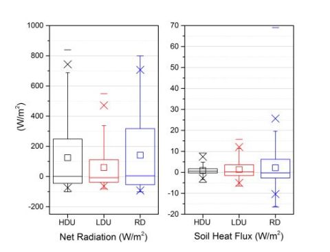

1. Introduction

Local climate is a function of upper atmospheric and boundary layer processes operating simultaneously at multiple scales. Global, synoptic, mesoscale, and microclimate processes intermingle resulting in observed local climate conditions [1]. Surface heating results in turbulence, which influences climate at each scale, and is influenced by roughness at the Earth's surface [1]. Surface characteristics include presence and size of water bodies, topography, and presence, amount, and type of vegetated cover [2]. Land use alters surface characteristics and hence atmospheric processes across spatial scales. Surface temperatures vary depending on land cover types, for example, agricultural cropland or natural shrubland [3]. Urban development is often accompanied by decreased vegetative cover, an increase in large impervious surface areas, and decreased albedo all of which increase surface absorptivity and therefore reemitted energy [4]. Ultimately, there is little argument that human alterations of the natural landscape by development of urban centers often result in some of the greatest alterations to local and regional climate regimes.

Air temperatures in urban areas have been shown to be significantly different than temperature measured in nearby rural areas. This trend is well documented in the literature, beginning with the seminal work of Howard [5]. Howard reported a disparity in the air temperatures of urban and rural sites, noting warmer daytime temperatures and cooler evening temperatures in the city [1]. Oke [6] used a model of the city as an island, which was distinguished from the surrounding rural area by isotherms similar to topographic contour lines. The gradient of urban and rural temperatures is often described by urban heat island intensity (UHII), which is an accepted index of the urban heat island (UHI) effect that quantitatively characterizes surface or atmosphere temperature alterations relative to rural surroundings [7].

Measurement of atmospheric and climatic variables in urban environments is challenging due to many factors including (but not limited to) distribution of precipitation, air temperature, relative humidity, wind speed, and soil temperature [1,8]. Each of these metrics are unevenly distributed in urban centers due to highly variable surface characteristics (as presented above), and may be heavily influenced by the level and type of human activity on a daily, weekly, or seasonal basis (e.g., traffic patterns during weekday rush hour) [2,3,8,9]. A number of methods have been proposed to resolve difficulties associated with collecting accurate microclimate data in urban environments, including comparison of data from nearby urban and rural sites, sampling from a variety of sites within a city, analyzing data from static climate stations pre- and post-development, and most recently by the use of satellite imagery [10]. Methods of data collection have advantages and disadvantages, and there has been a shift in recent years from analysis of data collected at monitoring stations to the use of satellite infrared imagery interpretation and/or simulation models [8,11,12]. The modal shift in data acquisition and data type is attributable to advances in available technology and the need for spatially representative measurements [12]. However, a great deal of research is needed using short and long-term data sets from terrestrial monitoring sites located in variably impacted urban settings to improve mechanistic understanding, and validate UHI model simulation predictions.

Urban heat island intensity is positively correlated with human population, though the strength of the correlation varies geographically. For example, distinct UHI differences between North American and European large cities are presumably attributable to higher average density of taller buildings in North American cities resulting in reduced sky view and greater heat intensities [6,13]. Two recent studies, one that analyzed satellite imagery and another that compared data pertaining to land use and surface characteristics with a population sprawl index of metropolitan areas in the United States, confirmed a similar relationship between size of an urbanized area and UHI effect [11,14]. The positive correlation becomes significant in predicting future heating effects of the UHI effect, as urban heating can be intensified by a warming climate, potentially impacting the health of people living in urban areas [14].

1.1. Alterations to Climate Variables

The urban heat island effect has been correlated to convective storm activity, and can therefore have varying effects on precipitation depending on atmospheric conditions. Convective storms may be initiated at the UHI convergence zone which is created through a combination of increased temperature and mechanical turbulence resulting from complex urban surface geometry and roughness [7,15]. Conversely, the clouds associated with a synoptic-scale front (e.g., stratiform cloud formations) may also separate, in effect moving laterally past the UHI [15]. The effect of UHI on precipitation can be further complicated by aerosols and pollution associated with urban areas, as particulates in the atmosphere provide condensation nuclei [7,16]. Nuclei can either initiate or suppress precipitation processes, and are not well understood. Other possible mechanisms for urban influences on precipitation can include low level destabilization due to thermal perturbations and local enhancements of moisture [7].

The impacts of urban climate alterations on the precipitation regime extend beyond the immediate boundaries of metropolitan areas [7]. Effects may extend downwind or interact with other metropolitan influences at a regional to global scale [7,16]. Incoming solar radiation drives surface and atmospheric heating, and is greatly influenced by the reflectance (albedo) of the Earth's surface at a given location [2]. Albedo is lowered in urban areas as natural vegetative cover is replaced with buildings and impermeable concrete and asphalt surface, resulting in greater absorption of incoming short-wave radiation [2]. The increased heat storage in the impervious surfaces is ultimately re-emitted as sensible heat [7]. The additional heat capacity of buildings in cities is one of the most significant factors contributing to the urban heat island effect [17]. Ultimately, additional research is needed to understand the implications of atmospheric alteration at all scales. Short and long-term climate data sets collected from multiple land use types across urban and rural gradients could provide necessary observed data to improve understanding of UHI processes and process alterations [17].

Solar radiation is not the only source of heat in the urban environment. Anthropogenic heat generated by vehicles, equipment, and industrial processes also contributes to UHII [18]. Unfortunately, natural cooling processes of evaporation and transpiration are often much reduced in part due to vegetation replacement with impervious surfaces. Recent studies showed that urban locations with a greater percentage of vegetated area are frequently cooler, as is a city with an overall greater percentage of vegetative cover density [2,18,19]. The magnitude of the heating effect in an urban heat island is also dependent upon the georgraphical location of the city. For example, Imhoff et al. [11] found that the relative UHII was greater if the city was located in a forested biome due to the greater cooling potential of the surrounding forest through evapotranspiration and interception of precipitation.

The relationship between relative humidity and UHII varies seasonally, but is generally negatively correlated [1,9]. Lower relative humidity in urban areas is a function of increased surface heating, air temperature, and lowered evapotranspiration due to less vegetative cover [1]. The presence, size, and location of water bodies in or near urban areas can also influence evaporation and hence relative humidity values [20]. The presence of buildings and other structures at the surface of the urban environment alters surface roughness and wind speed [18]. This effect is not limited to the atmosphere near the surface, but extends upward for potentially hundreds of meters [1,6]. At some threshold, an increase in wind speed at the mesoscale diminishes UHII as heat is moved away from the urban center by convection. Increased wind speeds can be positively correlated with cloud cover, which are both in turn negatively correlated with the UHI effect [9].

The temperature effect of UHI also manifests in the soil. Urban areas with elevated air temperatures resulting from UHI exhibit higher subsurface temperatures than rural areas [21]. The increase in subsurface temperature is a result of conduction of surface heat, and the effects may continue downward for several meters into the soil [22]. The extent and depth of soil heating is highly dependent on soil thermal properties, which are influenced by soil structure and texture and are therefore often highly variable between sites [21]. Previous studies showed that annual soil heating curves were of a similar shape seasonally. However, there is a distinct urban-rural temperature gradient [21]. Soil heating can also extend beyond urban boundaries, affecting temperatures in groundwater aquifers [23].

1.2. Objectives

The goal of the following work was to examine long-term climate data from a representative urban environment in the central U.S. to better understand the UHI effect in that distinct physiographic region. Objectives included: (a) comparison of long-term microclimate data collected at regionally representative urban and rural sites; (b) comparison of microclimate variables between nested urban sites of varying development intensity; and (c) comparison of surface heating (i.e., net radiation) and soil heat flux between nested urban sites. Results hold important implications for urban developers and planners and provide land managers with the science-based knowledge necessary to improve decision-making processes.

2. Methods

2.1. Study Sites and Instrumentation

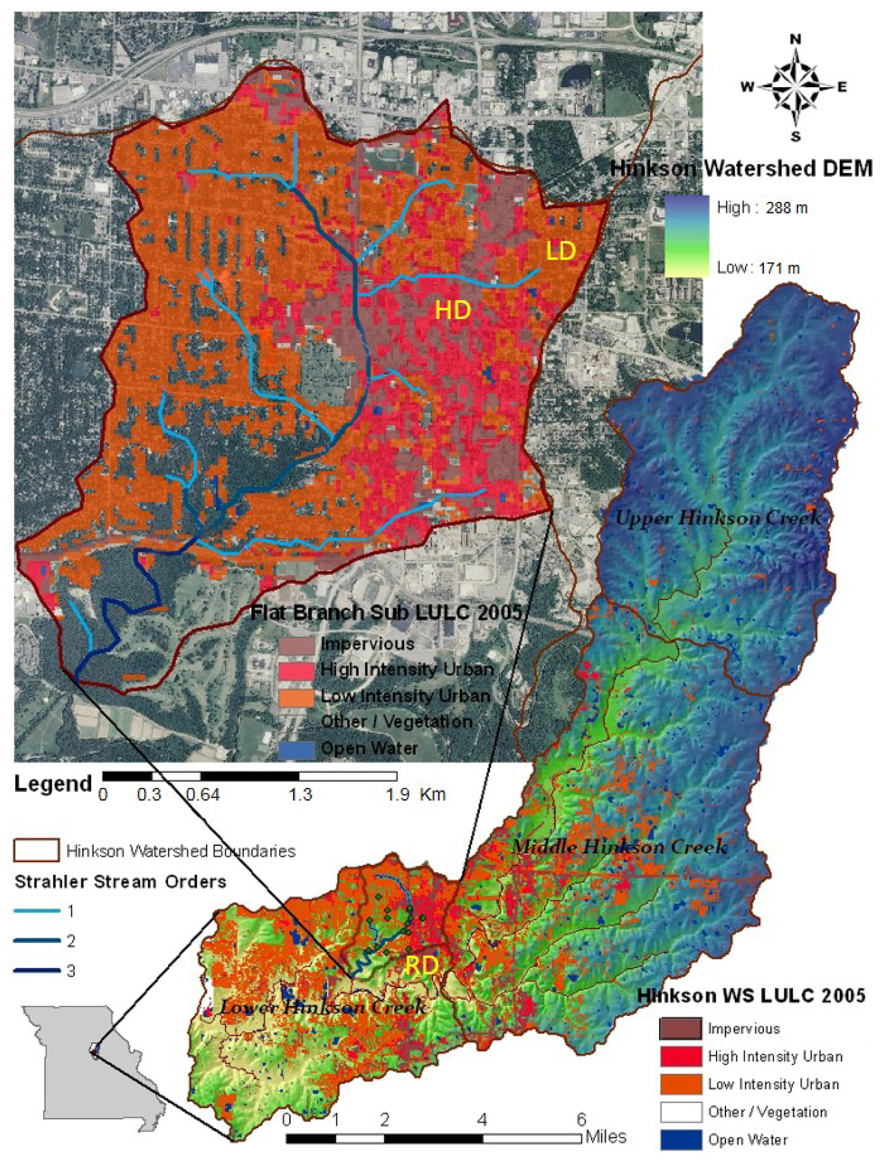
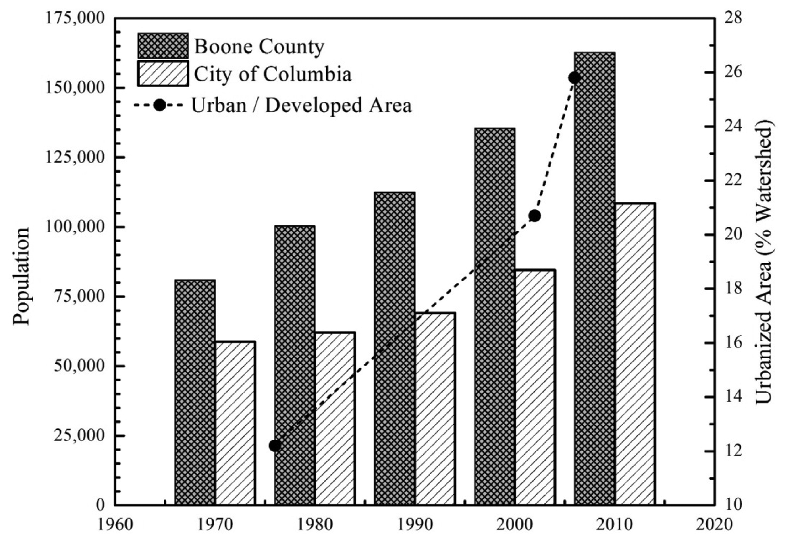
This study took place in the Hinkson Creek Watershed located in central Missouri, USA. The Hinkson Creek Watershed (HCW) includes more than 60% of the city of Columbia (population approximately 108,000) [24], and contains commercial, urban, and residential areas consisting predominately of impervious and high to low density urbanized areas [25]. The HCW is a representative urban watershed given its growing residential composition with progressive commercial expansion. Figure 1 shows a population growth trend that is very similar to other mid-sized cities in the Midwest US, and elsewhere. Land use in the watershed is approximately 25.8% forest, 49.8% cropland/grassland, and 15.8% urban area (

Table 1. Hinkson Creek Watershed Land Use/Land Cover Summary, source: Missouri Spatial Data Information Service (MSDIS).

Land Use/Cover	Area (Hectare)	Percentage
Impervious (Roads, Parking Lots)	1117.3	4.8
High Intensity Urban	517.7	2.2
Low Intensity Urban	3168.5	13.6
Barren or Sparsely Vegetated	32.2	0.1
Cropland/Grassland	11576.2	49.8
Forest	5996.9	25.8
Wetland	276.5	1.2
Open Water	562.2	2.4
Total	23247.4	100

).

Soil types in the Hinkson Creek Watershed range from thin cherty clay and silty to sandy clay in lower reaches to loamy till with a well-developed claypan in the uplands [26]. Two climate monitoring sites (urban and rural) were established in 1994 that supplied long-term time-series data for the current work. Sanborn Field (Figure 2) is located on the University of Missouri campus (38.942505° N, −92.320282° W), and is approximately centrally located within the city of Columbia. South Farm Agricultural Experiment Station (not shown) is located approximately four miles away (38.912474° N, −92.282292° W), in a rural area southeast of Columbia. The latter location was previously shown to exist outside the immediate influence of the city of Columbia UHI [17]. Both sites were equipped with instrumentation to measure a series of climate variables: precipitation (mm), air temperature (°C), relative humidity (%), wind speed (m/s), wind direction (degrees), incoming shortwave solar radiation (W/m²), soil temperature at 5 cm (°C), and soil temperature at 10 cm (°C) (

Table 2. Variables sensed and sensor model and manufacturer for urban gradient study sites in Columbia Missouri, USA. R and U indicate sensors used at Rural and/or Urban sites, respectively.

Variables Sensed	Sensor Model	Sensor Manufacturer
Precipitation	TE525 (R/U)	Texas Instruments
Air Temperature Air Temperature	CS207 (R) CS500, HC2S3 (R/U)	Fenwal Electronics Vaisala
Soil Temperature	CS 107s (R/U)	Campbell Scientific
Relative Humidity Relative Humidity	CS207 (R) CS500, HC2S3 (R/U)	Fenwal Electronics Vaisala
Wind Speed and Direction	014A, 04A, 034B (R/R/U)	Met-One
Short Wave Radiation	200x, 200s (R/R)	Li-Cor
Net Radiation	NR01 (U)	Hukseflux
Soil Heat Flux	HFP01SC (U)	Hukseflux

). Data were recorded at hourly intervals for the duration of the study period: 18 January 1995–8 October 2013.

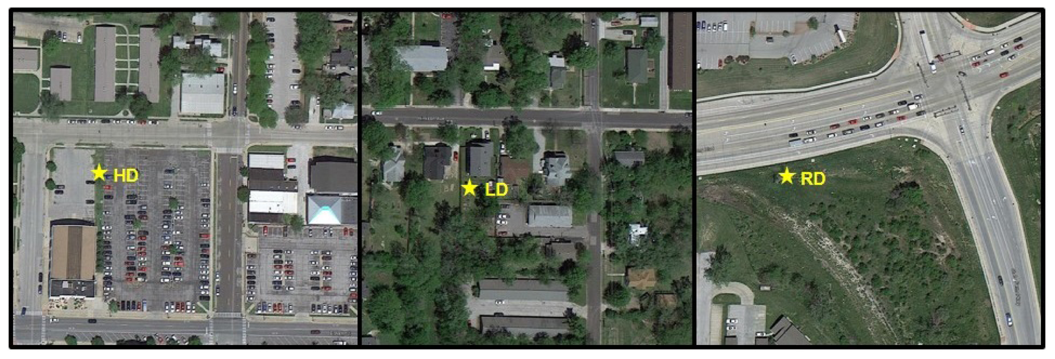
To better understand intra-urban UHI and development-related microclimatic gradient relationships, three monitoring sites were established within the city of Columbia in 2013 in varying land use types classified as low density urban, recent development, and high density urban (Figure 2). The low density urban site was located within a historic residential neighborhood in central Columbia (38.956418° N, −92.31506° W), characterized by more extensive and older vegetation (i.e., trees) and less impervious surface area relative to the other two sites. The recent development site was located in an area of progressive commercial expansion (38.909502° N, −92.326527° W), characterized by a mixture of remnant vegetation and newly constructed roadbeds, parking lots, and commercial buildings. The high density urban site was located in downtown Columbia (38.954228° N, −92.328876° W). The site contains little vegetation and is surrounded by extensive impervious surface area and buildings (Figure 3). Site land use characterizations and assignations are consistent with those proposed by MSDIS [25]. Each site was equipped with instrumentation to measure a series of microclimate variables including precipitation (mm), air temperature (°C), relative humidity (%), wind speed (m/s), wind direction (degrees), net solar radiation (W/m²), soil temperature at 2.5 and 15 cm (°C), and soil heat flux (W/m²). Data were collected and recorded at 30 min intervals from 2 June 2013 to 28 September 2013.

2.2. Urban Sites: Net Radiation and Soil Heat Flux

Considering the geographical proximity of the three intra-urban gradient monitoring sites, and their topographical similarity, it is reasonable to expect similar rates of incident shortwave radiation at the sites. Therefore, to analyze the presence, extent, and mechanistic processes of the UHI, it is important to consider the entire radiation budget (i.e., shortwave and longwave). Net radiation (W/m²) was measured at the three urban gradient monitoring sites using Campbell Scientific NR01 Four Component Net Radiation sensors. NR01 sensors combine two pyranometers, measuring incoming (in) and outgoing (out) shortwave radiation, and two pyrgeometers, measuring incoming and outgoing longwave radiation to calculate net radiation according to the equation:

$$\mathrm{R}\mathit{net}=(\mathrm{SW}\mathit{in}-\mathrm{SW}\mathit{out})+(\mathrm{LW}\mathit{in}-\mathrm{LW}\mathit{out})$$

(1)

where SW denotes shortwave (W/m²) and LW denotes longwave (W/m²) [27].

In addition to net radiation, soil heat flux and storage is an important consideration when analyzing urban energy budgets. If urban land uses impact net radiation budgets, the soil matrix directly reflects those alterations through altered rates of heat storage and remittance. Furthermore, land surface changes in the urban environment can affect reflectivity, absorptivity, and remittance of radiation. Therefore, comparing soil heat flux across the urban gradient may provide important information for understanding UHI processes. Soil heat flux (W/m²) was measured using Campbell Scientific HFP01SC self-calibrating soil heat flux plates. Each unit consists of a thermopile that measures the temperature gradient across the plate (installed at a depth of 8 cm), averaging thermocouples to measure temperature change in soil above the plate, and water content reflectometers (CS650, Campbell Scientific) to measure soil water content. Using these data, soil heat flux was calculated according to the equations:

$$S=\frac{\mathrm{\Delta }T{C}_{S}d}{t}$$

(2)

$$G_S=G_{8cm}+S$$

(3)

where S is the storage term, ΔT is the change in soil temperature above the plate, C_s is soil heat capacity, d is depth, t is time interval, G_s is heat flux at the surface, and G_8cm is heat flux at the sensor. Variables such as C_s require additional calculations including soil water content and soil temperature (not shown here). For other calculations, the reader is referred to Campbell Scientific Inc. (Logan, UT, USA) [28].

2.3. Data Analysis

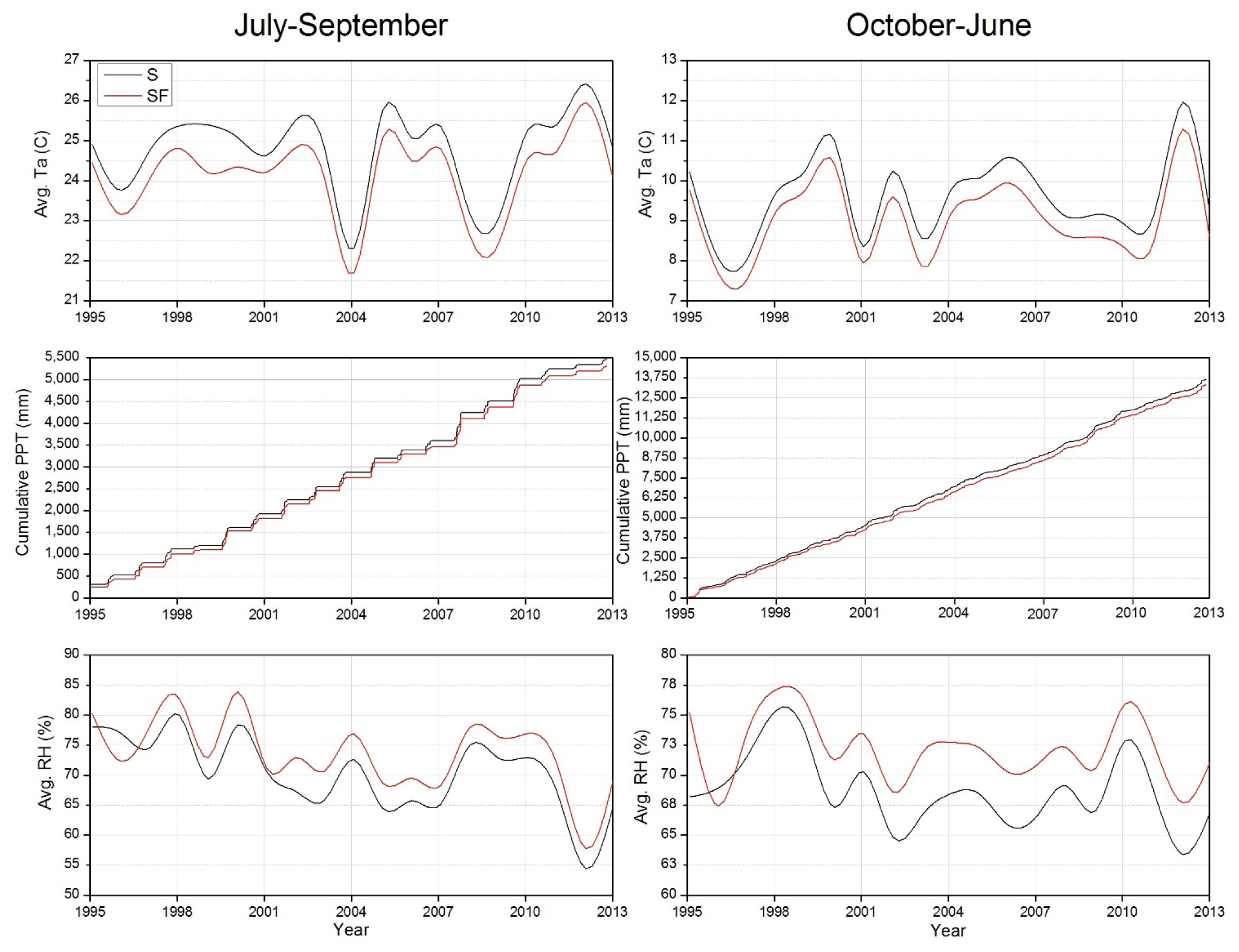
For all sites, descriptive statistics were generated for hourly climate data at each site and accompanied by one-way analysis of variance (ANOVA) to test for significant differences (p < 0.05) between sites. To test for the influence of autocorrelation on site differences, hourly data were aggregated to daily values, and subjected to the same suite of ANOVA tests. For the intra-urban gradient analysis, significant differences were followed with post hoc multiple comparison tests of specific means using Tukey's significant difference test [29]. Data gaps resulting from instrument error were filled using linear interpolation and simple linear regression (R² > 0.95). For urban–rural gradient data, to further highlight potential urban heat island effects, the study period was divided into summer months (21 June–19 September) when UHI effects are presumably greatest, and fall, winter, and spring months (20 September–19 June). Annual data were aggregated seasonally and analyzed using descriptive statistics and ANOVA. Site differences during the summer months were then compared to other sites/seasons to test for a seasonal impact on the UHI effect.

3. Results and Discussion

3.1. Long-Term Climate Trends

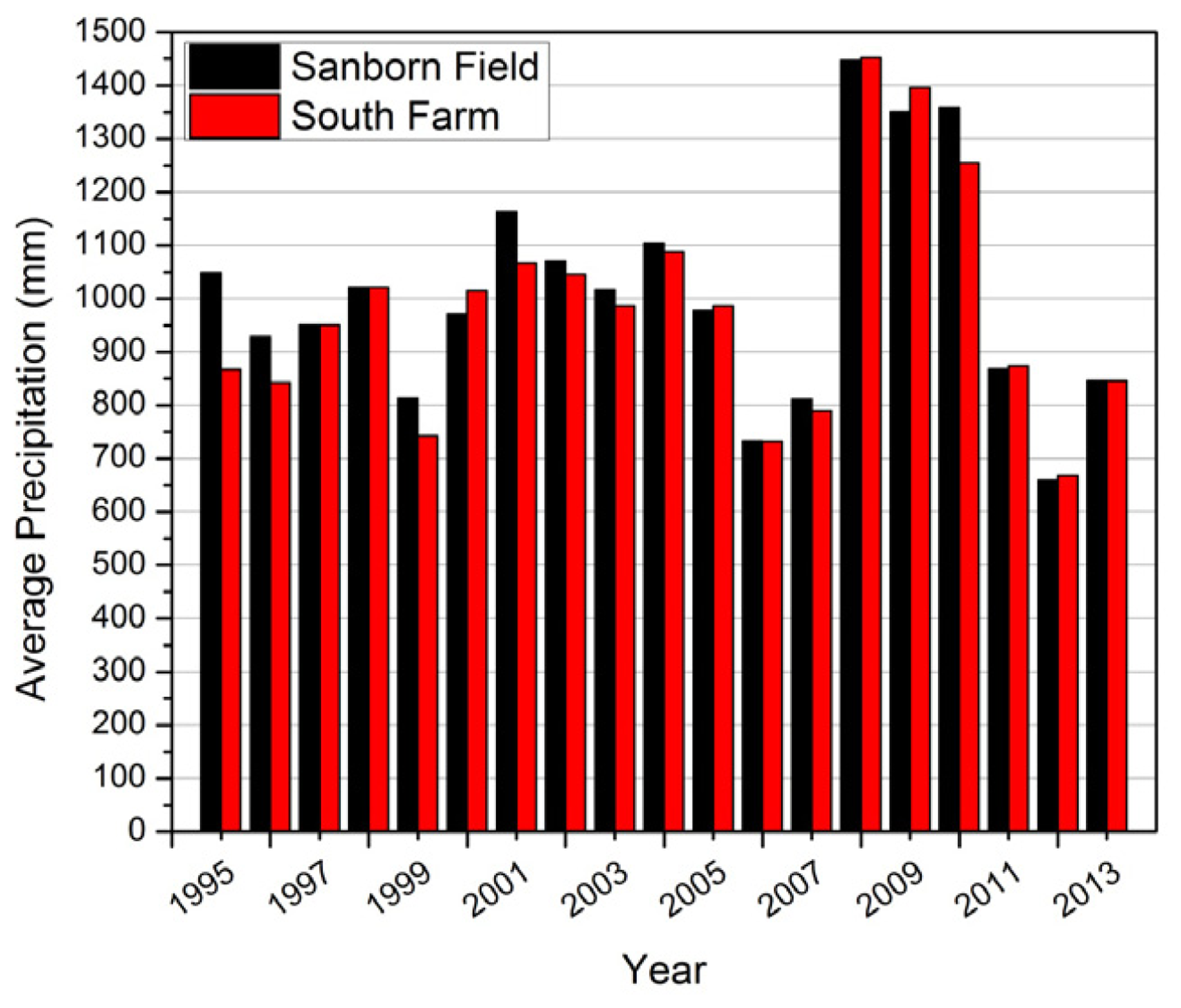
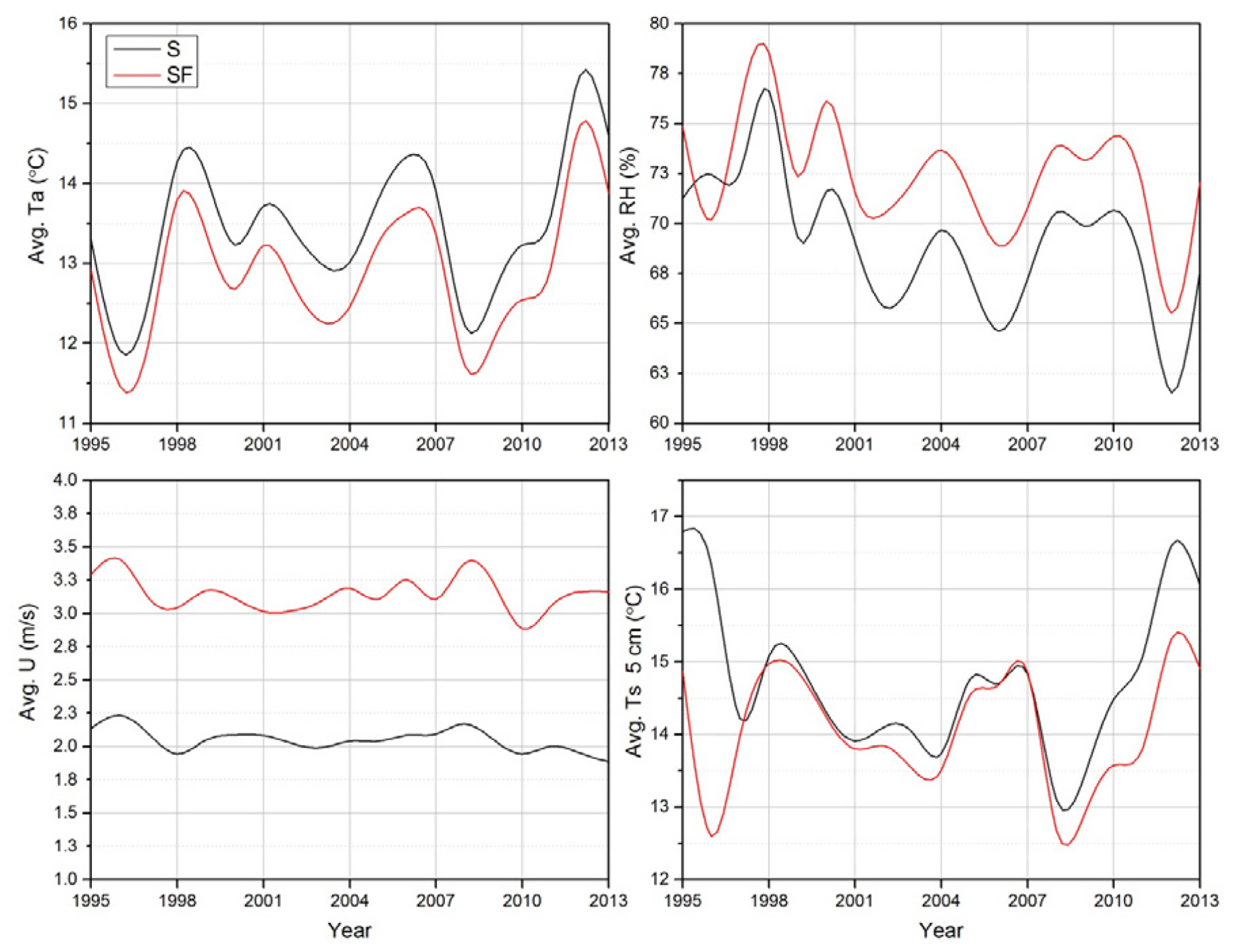
Climate analyses from Sanborn and South Farm monitoring sites exhibited distinct contrasts during the study period (

Table 3. Descriptive statistics of climate data at Sanborn and South Farm monitoring sites from 18 January 1995 to 8 October 2013, Columbia, Missouri, USA. PPT = precipitation, Ta = air temperature, RH = relative humidity, Usp = wind speed, Udir = wind direction, Rs = shortwave radiation, Ts = soil temperature.

Sanborn
Statistic	PPT (mm)	Ta (°C)	Rh (%)	Usp (m/s)	Udir (deg)	Rs (W/m2)	Ts 5 cm (°C)	Ts 10.2 cm (°C)
Avg.	19,137.47	13.47	69.11	2.05	172.59	168.54	14.75	14.63
Std. Dev.	0.97	11.16	19.08	1.09	94.48	255.14	10.45	9.88
Max.	45.21	41.90	100.00	21.10	-	1051.00	45.60	39.20
Min.	0.00	−25.20	12.00	0.00	-	0.00	−8.40	−8.83
South Farm
Avg.	18,626.90	12.89	72.51	3.15	179.63	169.59	14.07	14.25
Std. Dev.	0.93	11.10	18.36	1.73	96.39	252.73	10.46	9.35
Max.	42.42	41.70	100.00	12.96	-	1040.00	43.94	35.30
Min.	0.00	−26.30	2.00	0.00	-	0.00	−13.33	−4.88
% Diff.	2.74	4.53	4.92	53.47	4.08	0.62	4.84	2.66

Avg. = Average; Std. Dev = Standard Deviation; Max. = Max0imum; Min. = Minimum; % Diff. = Percent Difference.

). One-Way ANOVA results of hourly time series data indicated significant differences between the two sites (p < 0.001) for every climate variable except precipitation (p > 0.34) and average incoming solar radiation (p > 0.23). The statistical similarity of precipitation at the two sites is likely a result of the strong right-skewness of precipitation data. Precipitation data in the central US often demonstrate right-skewness since precipitation events are infrequent and variable. When zero values (no measurable precipitation) were removed from the data set, precipitation data exhibited similar patterns of right-skewness. After zero value removal, ANOVA results still indicated a lack of significant trend (p = 0.06) between the two sites. Notably, hourly time-series indicated 46 more precipitation events at Sanborn relative to South Farm during the study period. This supports the hypothesis that the UHI effect can lead to increased convective storm activity in urban environments. Although the difference in precipitation at the two sites was not statistically significant, statistical non-significance of climate data should not be assumed to be ecologically benign. The similarity of incoming shortwave solar radiation is reasonable considering the relatively close geographical proximity and topographical similarity (i.e., no prominent surrounding hills or landforms) of the two monitoring sites. During the 19 year study period, Sanborn was consistently warmer (average = 0.58 °C) and less humid (3.40%) than South Farm (Figure 4). This result is in agreement with numerous previous studies dating back to the work of Howard [5], and including that of Unger et al. in 2001 [8]. Howard was the first to catalog an air temperature gradient between rural and urban sites, but his work was limited to air temperature as a measure of the rural versus urban climate gradient [5]. Unger et al. analyzed air temperature variation at rural and urban sites near Szeged, Hungary, and described isolines corresponding to the urban land use intensity throughout their study area, with the highest temperatures being found in the center of the city [8]. The air temperature gradient identified in the present study is in agreement with Lupo et al. [30] who used twenty temperature sensors distributed throughout the greater Columbia, Missouri area as well as data from established climate stations over a period of one year, and noted a temperature gradient that correlated land use intensity with highest temperatures near the city center and a highly developed suburban area south of the city [30]. Ensuing work by Buckley et al. [17] helped to establish a limit on the areal influence of the UHI effect that was reported in the Lupo et al. [30] study. The urban versus rural relative humidity gradient in the present study, with a 3.40% lower relative humidity at the urban site, is in agreement with the negative correlation with the UHI effect identified by Papanastiou and Kittas in 2009 [9]. It is worth acknowledging that the absolute difference between average temperatures of the sites (0.58 °C) was near the accuracy of the air temperature sensor used (0.5 °C). Therefore, the difference between the sites, while significant (p < 0.05), should also be considered within the context of sensor accuracy. It is also worth noting that the Sanborn site lies in the middle of an inner city field often used for small scale agricultural crops (corn, soybeans, grass) by University of Missouri researchers. On this basis some UHI variables such as air temperature could be attenuated, and underestimated at certain times, and thus more similar to the South Farm site. Normally, relative humidity in urban areas is generally decreased as a result of reduction in vegetated cover and antecedent soil moisture conditions in combination with increased air temperature and surface heating [1].

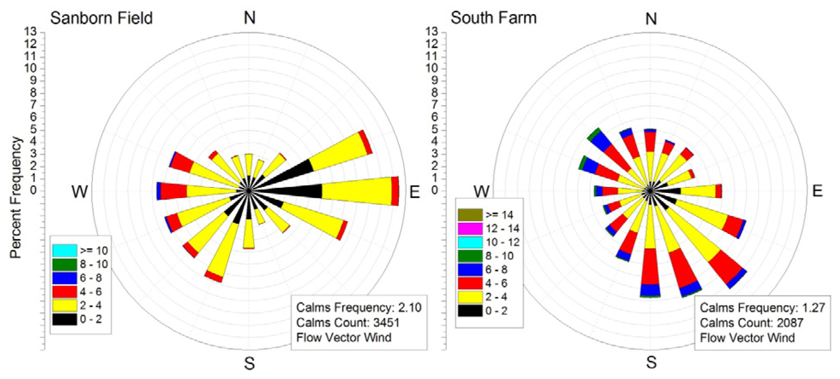
In the current work, the variable exhibiting the greatest difference between the two sites was average wind speed, which was more than 50% greater at South Farm (rural site). Conceivably, higher wind speeds could result in precipitation gauge undercatch at South Farm. Precipitation gauges were not shielded at either site. Therefore, and though speculative, observed precipitation differences in the current work may be underreported, and could be even greater if gauges were properly shielded. Lower wind speeds at the Sanborn Field site are presumably the result of greater surface complexity (i.e., buildings and structures) and the interruption of wind currents by buildings in the vicinity of the Sanborn site. Obstruction, diffusion, and redirection of turbulence by the greater urban surface roughness likely results in lower average wind speeds at the site. The observed wind speed gradient noted in the current work is corroborated in previous studies. In 2012, Papanastasiou and Kittas reported that wind speed was negatively correlated with the intensity of urban land use [9]. Ryu and Baik confirmed this relationship in 2012, showing that the urban geometry of buildings was a causative factor of urban wind speed reduction [18]. Ryu and Baik also showed a positive correlation between reduced wind speed in the urban environment and reduced daytime heat island intensity [18]. Figure 5 illustrates average wind direction at both sites. Analysis showed wind direction at both sites to be, on average, of southerly origin (Table 3). It is arguable that average wind direction data should indicate southerly direction regardless of geographic location. Therefore, to better characterize wind direction variability between Sanborn Field and South Farm, U (east-west direction) and V (south-north direction) wind components were calculated as per the methods of Stull [31]. For U average, minimum, maximum and standard deviation were 0.145°, −7.772°, 9.023° and 1.93° for the Sanborn site and 0.159°, −9.372°, 12.486°, and 2.391° for the South Farm site. For V, average, minimum, maximum and standard deviation were 0.141°, −4.999°, 6.395° and 1.277° for the Sanborn site and 0.376°, −10.970°, 10.973°, and 2.646° for the South Farm site. Using this method, average wind direction was estimated to be 225.8° for Sanborn and 202.9° for South Farm. These results further illustrate the disturbance of wind speed and direction in the urban environment, presumably attributable to presence of buildings and generally altered surface roughness.

While results show that average soil temperatures at both depths (5 and 10 cm) were greater at Sanborn Field relative to South Farm, Figure 4 illustrates the inconsistency of the trend during the study period. It is worth mentioning that while the 5 cm soil temperature measurements were collected at both sites under bare soil, the South Farm 10 cm soil temperature data were collected under a sod cover not present at the Sanborn site. Other site maintenance related issues (sensor degradation, debris, mowing) may have contributed to data trend inconsistencies. Despite vegetation (crop types) and management related cover differences (assumed a negligible effect over long-term), soil temperature data showed a gradient (5 cm depth: 14.75 and 14.07 °C for Sanborn and South Farm, respectively; 10 cm depth: 14.63 and 14.25 °C for Sanborn and South Farm, respectively) between rural and urban temperatures which was correlated with the air temperature gradient (13.47 and 12.89 °C of Sanborn and South Farm, respectively), and similarly equivalent attenuation of surface heating with increasing depth, consistent with results of previous studies [20,22,30,32]. Ferguson and Woodbury emphasized in 2007 that temperature effects of UHI at the surface are positively correlated with temperature effects of UHI at the subsurface [21]. Tang et al. (2011) also noted a positive correlation between soil temperature, air temperature and land use intensity, finding that the temperatures of urban soil were generally higher than those of rural soil [21].

Over the course of the present study, the Sanborn Field site received 510 mm more precipitation than South Farm (Figure 6) indicating a long term trend of greater precipitation at the more urbanized site (i.e., Sanborn). Bornstein and Lin reported an increased likelihood of thunderstorms arising at convergence zones between urban and rural land use types [15]. They also showed that moving thunderstorms can bifurcate and pass around urbanized areas [15]. The data in the current study indicate that Columbia, Missouri falls more generally into the first category, perhaps due to the fact that Columbia is a mid-sized city. A third possible mechanism for an urban influence on precipitation includes destabilization due to the UHI [7]. While it is difficult to generalize the aerosol effect on precipitation across seasons and atmospheric conditions, increased aerosol concentrations lead to decreased precipitation in stratocumulus clouds, small cumulus clouds, orographic clouds, cold-based convective clouds, and dry environment deep convective clouds [33,34]. Increased aerosol concentrations lead to increased precipitation in warm-based deep convective clouds, convective cloud ensembles and squall lines in moist environments [33,34]. With seasonal transition from summer to winter in Missouri, the portion of precipitation from stratocumulus and cold-based convective clouds increases while the portion of precipitation from warm-based deep convective clouds decreases. Furthermore, during winter a physical mechanism for aerosol transport to cloud level may generally be lacking due to less frequent convection and the absence of orographic influences. Therefore, although increased aerosol concentrations from an urban area can lead to both increases and decreases in precipitation, one would expect an aerosol effect on precipitation in Columbia, if discernable, to be that of increased precipitation during the warmer months within and downwind of the urban area.

3.2. Long-Term Climate Seasonal Analysis

ANOVA did not indicate a statistically significant seasonal difference, with significant differences between the two sites following the same pattern in each seasonal aggregate (e.g., summer vs. other seasons, see Methods) as in the general analysis (i.e., significant differences for all climate variables except precipitation and shortwave radiation). In general, this result shows the presence of the UHI effect during all seasons, an important finding that is also in agreement with previous studies such as that of Papanastiou and Kittas, who noted the UHI effect in summer and winter, though winter UHII was less than that of summer [9]. For example, maximum winter UHII was shown to be 3.4 °C, while the maximum UHII in summer was 3.1 °C [9]. Similarly, in the present study, quantitative contrasts between climate variables during the summer relative to differences during the fall, winter, and spring indicate a definable, if not statistically significant, seasonal influence on the UHI effect (

Table 4. Climate descriptive statistics recorded at Sanborn and South Farm monitoring sites during summer months (July–September) relative to fall through spring months (October–June), 18 January 1995–8 October 2013, Columbia, Missouri, USA. PPT = precipitation, Ta = air temperature, RH = relative humidity, Usp = wind speed, Udir = wind direction, Rs = shortwave radiation, Ts = soil temperature.

Sanborn: July–September
Statistic	PPT (mm)	Ta (°C)	RH (%)	Usp (m/s)	Udir (deg)	Rs (W/m2)	Ts 5 cm (°C)	Ts 10.2 cm (°C)
Avg.	5496.49	24.77	70.38	1.61	153.84	237.97	26.71	26.27
Std. Dev.	1.24	5.17	17.71	0.79	88.35	299.61	4.87	3.81
Max.	41.91	41.61	100.00	6.00	-	1037.00	45.60	39.20
Min.	0.00	5.22	13.00	0.00	-	0.00	10.22	13.40
South Farm: July–September
Avg.	5320.20	24.09	73.68	2.46	157.99	237.47	26.00	25.43
Std. Dev.	1.17	5.23	17.68	1.24	90.00	295.72	4.81	2.79
Max.	42.42	40.80	100.00	9.00	-	1031.00	43.94	35.30
Min.	0.00	−17.67	2.00	0.00	-	0.00	9.10	14.70
% Diff.	3.31	2.85	4.69	53.09	2.70	0.21	2.73	3.29
Sanborn: October–June
Avg.	13640.98	9.59	68.67	2.20	179.03	144.70	10.64	10.64
Std. Dev.	0.86	9.96	19.50	1.14	95.65	233.24	8.51	7.99
Max.	45.21	34.50	100.00	9.39	-	1051.00	39.80	36.06
Min.	0.00	−25.11	12.00	0.00	-	0.00	−8.40	−8.83
South Farm: October–June
Avg.	13306.70	9.04	72.11	3.38	187.07	146.28	9.97	10.41
Std. Dev.	0.82	9.92	18.57	1.81	97.38	231.62	8.56	7.55
Max.	39.88	34.00	103.81	12.96	-	1040.00	42.67	30.50
Min.	0.00	−23.40	13.00	0.00	-	0.00	−13.33	-4.88
% Diff.	2.51	6.07	5.00	53.56	4.49	1.09	6.74	2.14

Avg. = Average; Std. Dev. = Standard Deviation; Max. = Max0imum; Min. = Minimum; % Diff. = Percent Difference.

, Figure 7). For example, the percent difference between precipitation at Sanborn and South Farm (Sanborn > South Farm) was 3.31% during the summer and 2.51% during the rest of the year. Figure 7 showed a distinct stair-step pattern for cumulative precipitation during the summer months relative to the more gradually increasing line of precipitation during the fall, winter, and spring. This relationship is likely the result of fewer precipitation events during the summer, that are more intense, localized and convective versus more measureable events during the other three seasons, that are lighter, more uniform and widespread (Table 4). Actual difference between Sanborn and South Farm air temperature and soil temperature at both soil depths was greater during the summer relative to the fall, winter, and spring (0.68, 0.71, and 0.84 °C for air, 5 cm, and 10 cm soil temperature, respectively, during the summer as compared to 0.55, 0.67, and 0.23 °C during the fall, winter, and spring). These results indicate a greater difference between microclimate at the two sites during the summer, thus supporting a seasonal influence on the UHI effect.

3.3. Intra-Urban Gradient Analysis

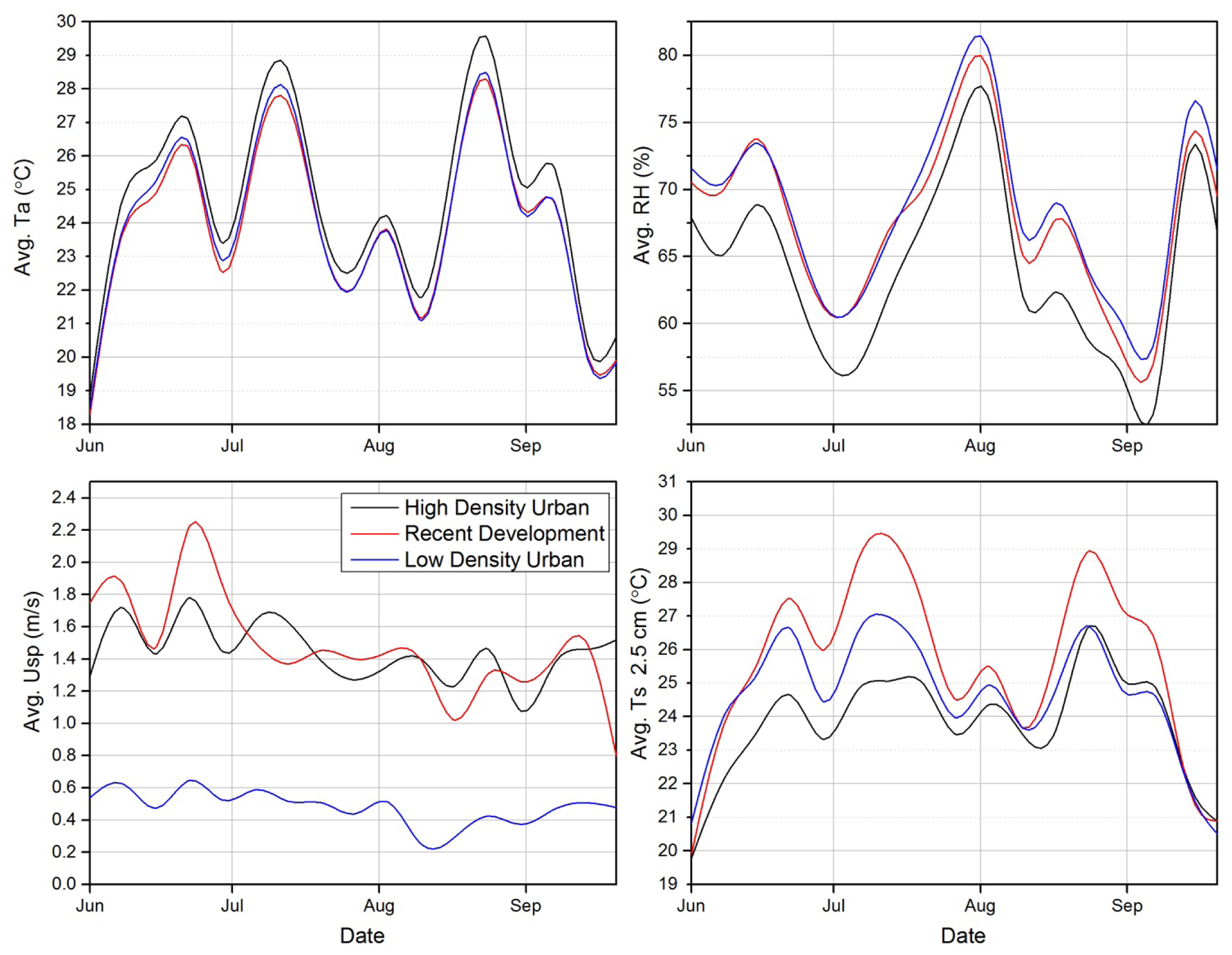
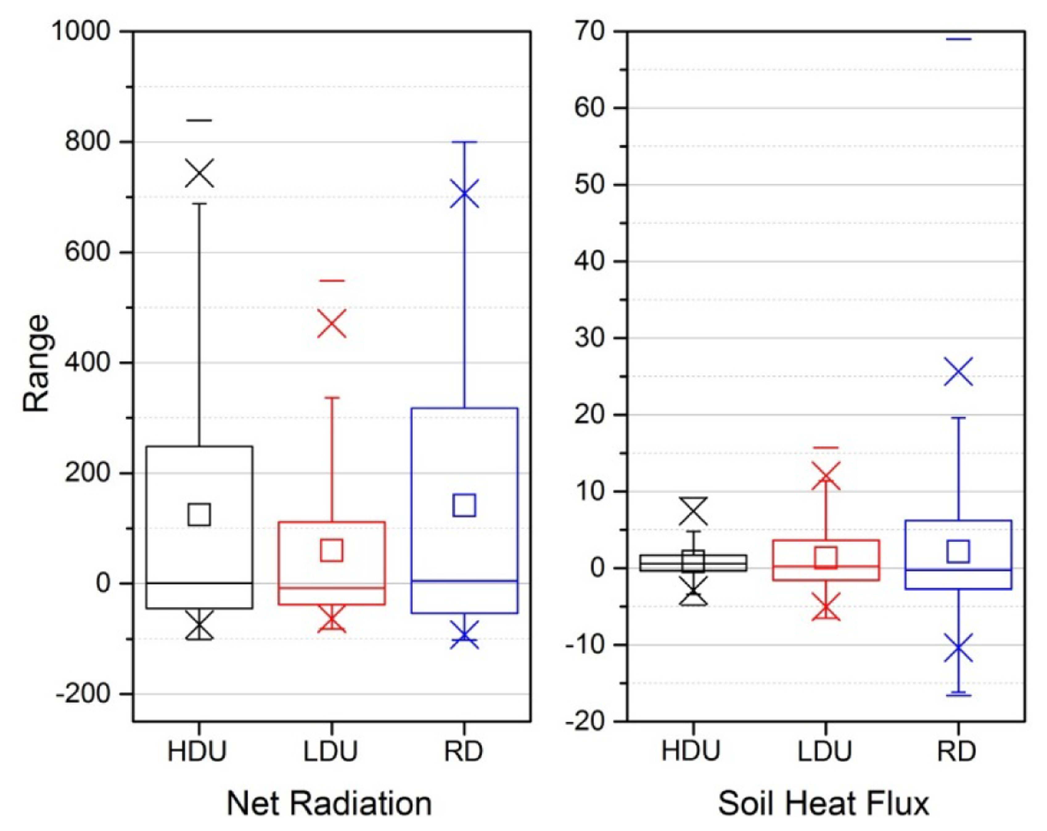
Results from analysis of the UHI intra-urban gradient study sites indicate a distinct impact of increasing urban development on microclimate (

Table 5. Climate results at low density urban, recent development, and high density urban gradient monitoring sites from 2 June 2013 to 28 September 2013, Columbia, Missouri, USA. PPT = precipitation, Ta = air temperature, RH = relative humidity, Usp = wind speed, Udir = wind direction, Rn = net radiation, Ts = soil temperature, SHF = soil heat flux.

Low Density Urban
Statistic	PPT (mm)	Ta (°C)	RH (%)	Usp (m/s)	Udir (Deg)	Rn (W/m2)	Ts 2.5 cm (°C)	Ts 15 cm (°C)	SHF (W/m2)
Avg.	204.70	23.78	68.82	0.48	164.62	60.12	24.50	24.16	1.34
Std. Dev.	0.49	5.15	17.82	0.40	80.64	145.21	2.43	1.92	3.93
Max.	15.40	37.72	99.30	1.88	354.20	548.70	31.08	28.35	15.72
Min.	0.00	8.81	27.34	0.00	0.10	−81.80	18.17	18.87	−6.50
% Diff. (L/R)	3.02	0.39	1.54	206.75	1.06	135.55	3.94	3.55	61.22
Recently Developed
Avg.	198.70	23.69	67.77	1.47	162.89	141.61	25.46	25.01	2.15
Std. Dev.	0.45	5.23	18.06	0.85	89.75	242.48	3.64	2.85	7.59
Max.	15.70	37.83	98.30	6.57	357.50	800.00	39.22	31.51	69.01
Min.	0.00	8.38	24.73	0.00	0.00	−102.00	16.14	17.61	−16.61
% Diff. (R/H)	1.69	3.36	5.46	2.13	6.89	13.66	7.44	6.13	153.23
High Density Urban
Avg.	195.40	24.49	64.27	1.44	174.12	124.59	23.70	23.57	0.85
Std. Dev.	0.46	5.05	17.17	0.63	97.55	223.79	2.02	1.56	1.94
Max.	14.50	37.30	97.90	4.23	357.80	839.00	30.02	26.39	9.17
Min.	0.00	9.39	25.80	0.00	0.00	−100.90	17.53	18.32	−4.80
% Diff. (H/L)	4.76	2.96	7.08	200.35	5.77	107.24	3.37	2.49	57.07

Avg. = Average; Std. Dev. = Standard Deviation; Max. = Max0imum; Min. = Minimum; % Diff. = Percent Difference; (L/R) = Low Density/Rural; (R/H) = Rural/High Density; (H/L) = High Density/Low Density.

, Figure 8), thus greatly supporting the hypothesis explaining the rural to urban gradient stated earlier. Results of One-Way ANOVA showed significant differences (p < 0.001) between the three sites for every variable except precipitation (p > 0.97). Tukey post hoc tests, which compare individual sites to one another, showed that for each significantly different variable except air temperature and wind direction, each site was significantly different (p < 0.05) from other sites. For air temperature and wind direction, the low density urban and recent development sites were not statistically significantly different. Average air temperatures were 23.69, 23.78, and 24.49 °C for the recently developed, low density urban, and high density urban sites, respectively. Previous studies such as that of Hart and Sailor suggested a gradient of air temperature from rural to increasingly more urbanized areas where the lowest temperatures occur in the rural area, increasing to a maximum near the city center [2]. Heterogeneity within this general pattern can occur as a function of the number of roads (i.e., increased impervious surface; increased air temperature), or vegetated areas in the city such as parks (i.e., decreased impervious surface; decreased temperature). Montávez et al. discussed a similar gradient in urban temperatures which increased with proximity to the city center in Granada, Spain [10]. The higher temperatures at the high density site in the current study are consistent with observations from previous studies. Relative humidity percent differences were 1.54%, 5.46%, and 7.08% for low density vs. recently developed, recently developed vs. high density, and high density vs. low density, respectively, with relative humidity decreasing as land use intensity increases. Similarly, Papanastiou and Kittas noted a negative correlation between relative humidity and land use intensity in winter (correlation coefficient −0.31), but found a weaker positive correlation in summer (correlation coefficient 0.17) [9]. The large difference in average wind speed at the low density urban site (approximately double) relative to the other sites is likely a result of increased turbulence and dissipation of kinetic energy by trees, buildings and fences located near the sensor. Analysis of net radiation showed significant (p < 0.001) differences between the three sites. The low density urban site had the lowest average net radiation (60.12 W/m²); the recently developed site had the highest value (141.61 W/m²). These results reflect differences in surface cover including presence and density of trees and grass (low density urban site), or asphalt and concrete (high density urban site). Zell and Hubbart suggested that a surface energy balance approach could be used to quantitatively assess ecosystem stability [35]. It was proposed that ecosystem stability is approached when all energy requirements are met or the net energy flux is always negligibly positive (i.e., net exergy) [35]. The results of the current work support the work of Zell and Hubbart in that the high density urban and the recently developed site had much higher net radiation relative to the low density site that was characterized by more trees and green spaces, and thus could be arguably more ecologically stable. Future work should investigate the usefulness of the surface energy balance ecosystem stability approach to target urban areas for conservation activities (e.g., urban forests) that may offset the UHI effect.

Soil heat flux averages at the low density, recently developed, and high density urban sites were 1.34, 2.15, and 0.85 W/m², respectively (Figure 9). Interestingly, the recently developed site showed the greatest and most variable rates of soil heat flux of the three sites. This is likely a result of soil conditions at the site. While the recent development monitoring station is in an area of commercial expansion, the soil where the sensors were installed is relatively undisturbed in a former agricultural field. It is worth noting that the recently developed site is surrounded on all sides by asphalt and that while it is unlikely that soil heat conduction is significant, advected heat from surrounding differentially heated surfaces (roads, parking lots) could alter local conditions resulting in similar microclimate attributes as the high density site. In comparison, the greatest disturbed soil (high density urban) showed the lowest and least variable rates of soil heat flux, indicating a surface nearing equilibrium in terms of heat absorption and reemission. Soil heat flux could have been attenuated somewhat at this site by the presence of a single tree that may have provided some shading. However, given the results, it is interesting to consider that highly urbanized impervious areas (e.g., asphalt and concrete cover) may more closely resemble black bodies in terms of more effective absorption and emission of energy.

Soil heat flux results hold important implications for the study of subsurface UHI effect. Uchida et al. [36], Tanguichi et al. [37], and Taylor and Stefan [38] studied the impact of urbanization on the thermal regime of shallow groundwater aquifers noting increased surface heating as the probable mechanistic cause for observed changes in shallow groundwater temperature. Conversely, Menberg et al. [23] identified engineered subsurface structures (e.g., sewers, basements) as the primary origins of increased subsurface temperatures in Karlsruhe, Germany. If increased surface heating is the cause of the observed changes in urban subsurface temperatures, then more urbanized sites would likely show higher rates of soil thermal loading (i.e., greater propagation of heat from the surface to the subsurface) relative to less urbanized sites. However, results of the current work show the high density urban site to exhibit the lowest rates of surface-to-subsurface thermal loading. Rather, barring site specific differences, it would seem possible that impervious materials such as asphalt and concrete may alter the reflectivity, absorptivity, and emissivity of the urban surface, resulting in lower rates of thermal loading to the subsurface. Furthermore, it is likely that reduced infiltration of water into urban soils, an effect of impervious surfaces (compaction, cover changes), contributes to this trend through reduced advected heat transport into the subsurface. These results illustrate the need for replication of studies and study sites such as those of the current work.

4. Summary and Conclusions

Previous research showed that changes in land cover and surface characteristics associated with urban land uses result in alterations of urban microclimate, commonly referred to as the Urban Heat Island effect or UHI. Increased air temperatures relative to rural or undeveloped regions, reductions in relative humidity, alterations of precipitation patterns via increased convective storm activity, disruptions of wind currents, and alterations to subsurface thermal regimes have all been linked to increased urban land use. To improve mechanistic understanding of UHI processes in the central US, a study was implemented in Columbia, Missouri, USA.

Data were collected at a representative urban (Sanborn) and rural (South Farm) site from 18 January 1995 to 8 October 2013 and compared to investigate long-term general UHI patterns in the region. Results showed significant differences (p < 0.001) between average air temperature (13.47 and 12.89 °C, at urban and rural sites, respectively); relative humidity (69.11% and 72.51%, at urban and rural sites, respectively); average wind speed (2.05 and 3.15 m/s at urban and rural sites, respectively); soil temperature at 5 cm (14.75 and 14.07 °C, at urban and rural, respectively) and 10 cm (14.63 and 14.25 °C, at urban and rural sites, respectively). Average wind direction at both sites was shown to be southerly in origin. The urban site received 510 mm more precipitation than the rural site during the study period. Data were aggregated on a seasonal basis (summer vs. fall, winter, and spring) and analyzed to test for a seasonal influence on the UHI effect. Significant differences between the two sites during each seasonal aggregate followed the same patterns as in the general analysis, indicating that the UHI effect occurs during all seasons.

Data were collected at a low density urban, recently developed, and high density urban site from 2 June 2013 to 28 September 2013 to investigate the presence of a UHI gradient related to urban land use intensity. Results showed significant differences (p < 0.001) between the three sites for every variable except precipitation. Results from the analysis of net radiation and soil heat flux at the three sites suggest significant alterations in urban energy budgets due to land use intensity. Although the low density urban site showed the lowest net radiation (60.12 W/m²), the high density urban site exhibited the lowest soil heat flux (0.85 W/m²) clearly indicating the energy budget heterogeneity of variously developed urban areas. Results of the current work hold important implications for urban planners and land managers seeking to improve decision making with science-based knowledge, and highlight the need for continued research on the impacts of urban land use gradients on energy budgets to improve mechanistic understanding of the urban heat island effect.

References

- Landsberg, H.E. The Urban Climate; Academic Press: New York, NY, USA, 1981. [Google Scholar]
- Hart, M.A.; Sailor, D.J. Quantifying the influence of land-use and surface characteristics on spatial variability in the urban heat island. Theor. Appl. Climatol. 2009, 95, 397–406. [Google Scholar]
- Jin, M.S. Developing an index to measure urban heat island effect using satellite land skin temperature and land cover observations. J. Clim. 2012, 25, 6193–6201. [Google Scholar]
- Arnfield, A.J. Two decades of urban climate research: A review of turbulence, exchanges of energy and water, and the urban heat island. Int. J. Climatol. 2003, 23, 1–26. [Google Scholar]
- Howard, L. Climate of London Deduced from Meteorological Observations, 3rd ed.; Harvey and Darton: London, UK, 1833. [Google Scholar]
- Oke, T.R. The energetic basis of the urban heat island. Q. J. R. Meteorl. Soc. 1982, 108, 1–24. [Google Scholar]
- Shepherd, J.M. A review of current investigations of urban-induced rainfall and recommendations for the future. Earth Interact. 2005, 9, 1–27. [Google Scholar]
- Unger, J.; Sümeghy, Z.; Gulyás, Á.; Bottyán, Z.; Mucsi, L. Land-use and meteorological aspects of the urban heat island. Meteorol. Appl. 2001, 8, 189–194. [Google Scholar]
- Papanastasiou, D.K.; Kittas, C. Maximum urban heat island intensity in a medium-sized coastal Mediterranean city. Theor. Appl. Climatol. 2012, 107, 407–416. [Google Scholar]
- Montávez, J.P.M.; Rodríguez, A.; Jiménez, J.I. A study of the urban heat island of Granada. Int. J. Climatol. 2000, 20, 899–911. [Google Scholar]
- Imhoff, M.L.; Zhang, P.; Wolfe, R.E.; Bounoua, L. Remote sensing of the urban heat island effect across biomes in the continental USA. Remote Sens. Environ. 2010, 114, 504–513. [Google Scholar]
- Mirzaei, P.A.; Haghighat, F. Approaches to study urban heat island–abilities and limitations. Build. Environ. 2010, 45, 2192–2201. [Google Scholar]
- Torok, S.J.; Morris, C.J.; Skinner, C.; Plummer, N. Urban heat island features of southeast Australian towns. Aust. Meteorol. Mag. 2001, 50, 1–13. [Google Scholar]
- Stone, B.; Hess, J.J.; Frumkin, H. Urban form and extreme heat events: Are sprawling cities more vulnerable to climate change than compact cities? Environ. Health Perspect. 2010, 118, 1425–1428. [Google Scholar]
- Bornstein, R.; Lin, Q. Urban heat islands and summertime convective thunderstorms in Atlanta: Three case studies. Atmos. Environ. 2000, 34, 507–516. [Google Scholar]
- Grimm, N.B.; Foster, D.; Groffman, P.; Grove, J.M.; Hopkinson, C.S.; Nadelhoffer, K.J.; Pataki, D.E.; Peters, D.P. The changing landscape: Ecosystem responses to urbanization and pollution across climatic and societal gradients. Front. Ecol. Environ. 2008, 6, 264–272. [Google Scholar]
- Buckley, P.I.; Market, P.S.; Lupo, A.R.; Fox, N. Further studies of the heat island associated with a small midwestern city. Atmos. Sci. Lett. 2008, 9, 226–230. [Google Scholar]
- Ryu, Y.H.; Baik, J.J. Quantitative analysis of factors contributing to urban heat island intensity. J. Appl. Meteorol. Clim. 2012, 51, 842–854. [Google Scholar]
- Hamdi, R.; Schayes, G. Sensitivity study of the urban heat island intensity to urban characteristics. Int. J. Climatol. 2008, 28, 973–982. [Google Scholar]
- Hathway, E.A.; Sharples, S. The interaction of rivers and urban form in mitigating the Urban Heat Island effect: A UK case study. Build. Environ. 2012, 58, 14–22. [Google Scholar]
- Tang, C.S.; Shi, B.; Gao, L.; Daniels, J.L.; Jiang, H.T.; Liu, C. Urbanization effect on soil temperature in Nanjing, China. Energy Build. 2011, 43, 3090–3098. [Google Scholar]
- Ferguson, G.; Woodbury, A.D. Urban heat island in the subsurface. Geophys. Res. Lett. 2007, 34, L23713. [Google Scholar] [CrossRef]
- Menberg, K.; Blum, P.; Schaffitel, A.; Bayer, P. Long-Term Evolution of Anthropogenic Heat Fluxes into a Subsurface Urban Heat Island. Environ. Sci. Technol. 2013, 47, 9747–9755. [Google Scholar]
- United States Census Bureau (USCB), 2011. U.S. Census Bureau Delivers Missouri's 2010 Census Population Totals, including First Look at Race and Hispanic Origin Data for Legislative Redistricting. Available online: http://2010.census.gov/news/releases/operations/cb11-cn49.html (accessed on 22 March 2011).
- MSDIS (Missouri Spatial Data Information Service), 2005. MSDIS Data Theme Listing. Available online: http://msdis.missouri.edu/datasearch/ThemeList.jsp (accessed on 11 October 2013).
- Chapman, S.; Omernik, J.; Griffith, G.; Schroeder, W.; Nigh, T.; Wilton, T. Ecoregions of Iowa and Missouri (Color Poster with Map, Descriptive Text, Summary Tables, and Photographs); US Geological Survey: Reston, VA, USA, 2002. [Google Scholar]
- Campbell Scientific Incorporated. NR01 Four-Component Net Radiometer Sensor. Available online: http://s.campbellsci.com/documents/us/manuals/nr01.pdf (accessed on 11 October 2013).
- Campbell Scientific Incorporated. Model HFP01SC Self-Calibrating Soil Heat Flux Plate. Available online: http://s.campbellsci.com/documents/us/manuals/hfp01sc.pdf (accessed on 11 October 2013).
- Smith, R. The Effect of Unequal Group Size on Tukey's HSD Procedure. Psychometrika 1971, 36, 31–34. [Google Scholar]
- Lupo, A.R.; Market, P.S.; Akyüz, F.A.; Guinan, P.E.; Lam, J.E.; Oravetz, A.M.; Maune, W.C. The Columbia, Missouri, Heat Island Experiment (COHIX): The Influence of a Small City on Local Surface Temperature Distributions and Implications for Local Forecasts. Electron. J. Oper. Meteorol. 2003, 4, 1–14. [Google Scholar]
- Stull, R. Meteorology for Scientists and Engineers, 2nd ed.; Brooks Cole Thomson Learning: Pacific Grove, CA, USA, 2000. [Google Scholar]
- Brady, N.; Weil, R. The Nature and Properties of Soils, 14th ed.; Pearson Education Inc.: Upper Saddle River, NJ, USA, 2008. [Google Scholar]
- Rosenfeld, D.; Givati, A. Evidence of orographic precipitation suppression by air pollution-induced aerosols in the western United States. J. Appl. Meteorol. Clim. 2006, 45, 893–911. [Google Scholar]
- Khain, A.P.; BenMoshe, N.; Pokrovsky, A. Factors determining the impact of aerosols on surface precipitation from clouds: An attempt at classification. J. Atmos. Sci. 2008, 65, 1721–1748. [Google Scholar]
- Zell, C.; Hubbart, J.A. A framework linking biophysical processes and resilience theory. Ecol. Model. 2013, 248, 1–10. [Google Scholar]
- Uchida, Y.; Sakura, Y.; Taniguchi, M. Shallow subsurface thermal regimes in major plains in Japan with reference to recent surface warming. Phys. Chem. Earth 2003, 28, 457–466. [Google Scholar]
- Taniguchi, M.; Uemura, T.; Jago-on, K. Combined effects of urbanization and global warming on subsurface temperature in four Asian cities. Vadose Zone J. 2007, 6, 591–596. [Google Scholar]
- Taylor, C.A.; Stefan, H.G. Shallow Groundwater temperature response to climate change and urbanization. J. Hydrol. 2009, 375, 601–612. [Google Scholar]