Real-Time Wavelet-Based Coordinated Control of Hybrid Energy Storage Systems for Denoising and Flattening Wind Power Output


Abstract
:1. Introduction

| Literature | Filtering method | Storage type | SOC regulation | Interconnection requirement | Real-time or hardware test |
|---|---|---|---|---|---|
| Ushiwata [6] | SMA | EDLC | X | X | X |
| Tanabe [7] | SMA | Battery | X | O | X |
| Sheikh [8] | SMA + EMA | SMES | X | X | X |
| Yoshimoto [9] | First order lag filter | Battery | O | X | X |
| Li [10] | SMA | Battery/EDLC | X | X | O |
| Suvire [11] | Fuzzy logic + SMA | Flywheel | X | X | X |
| Mishra [12] | Bacteria foraging | Battery | X | X | X |
| Li [13] | Fuzzy logic + wavelet | Battery | O | X | X |
| Jiang [14] | Online wavelet | Battery/EDLC | O | O | X |
| Proposed | Online wavelet | Battery/EDLC | O | O | O |
2. Wind-Hybrid Energy Storage System Modeling in RSCAD
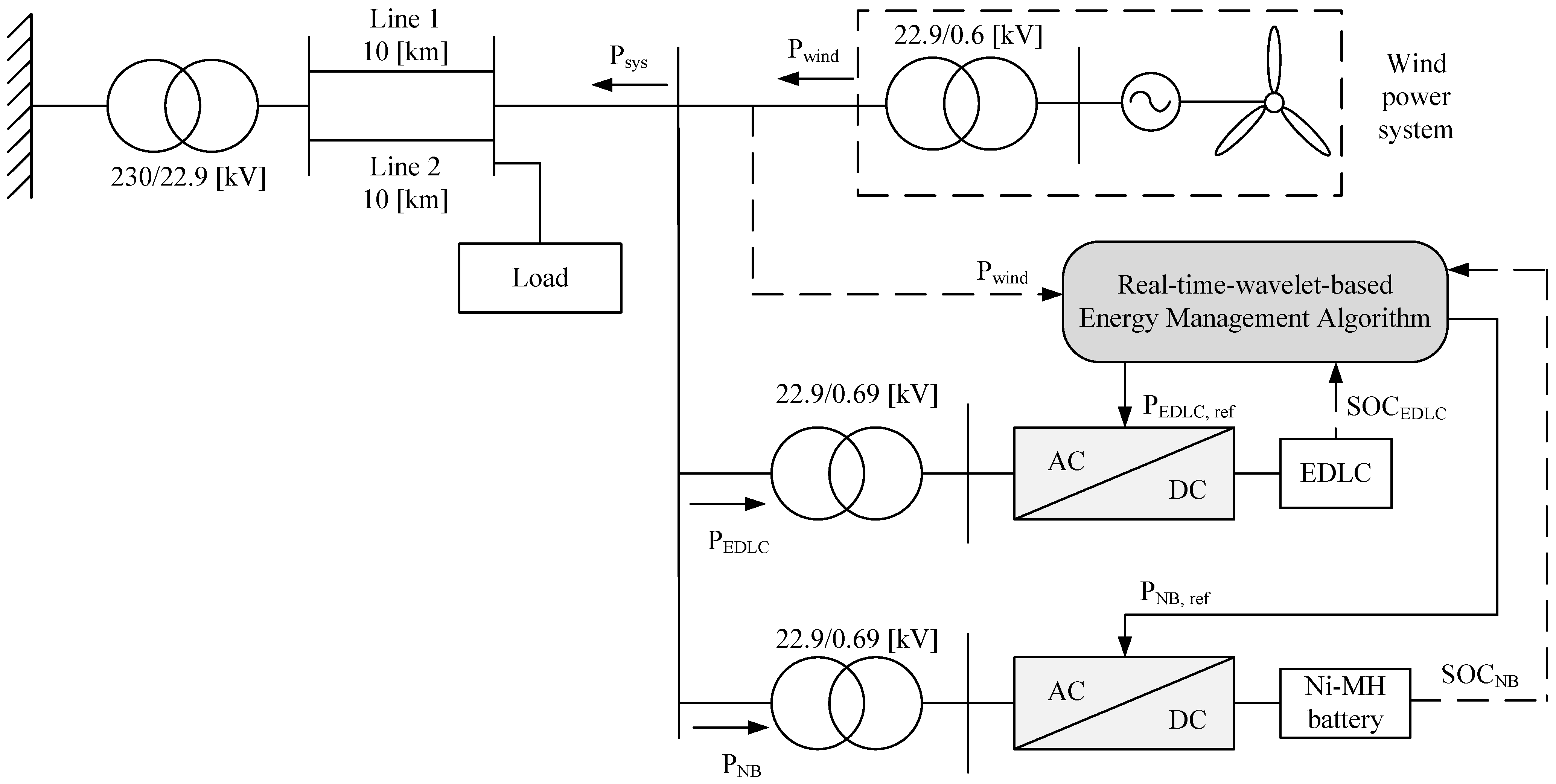
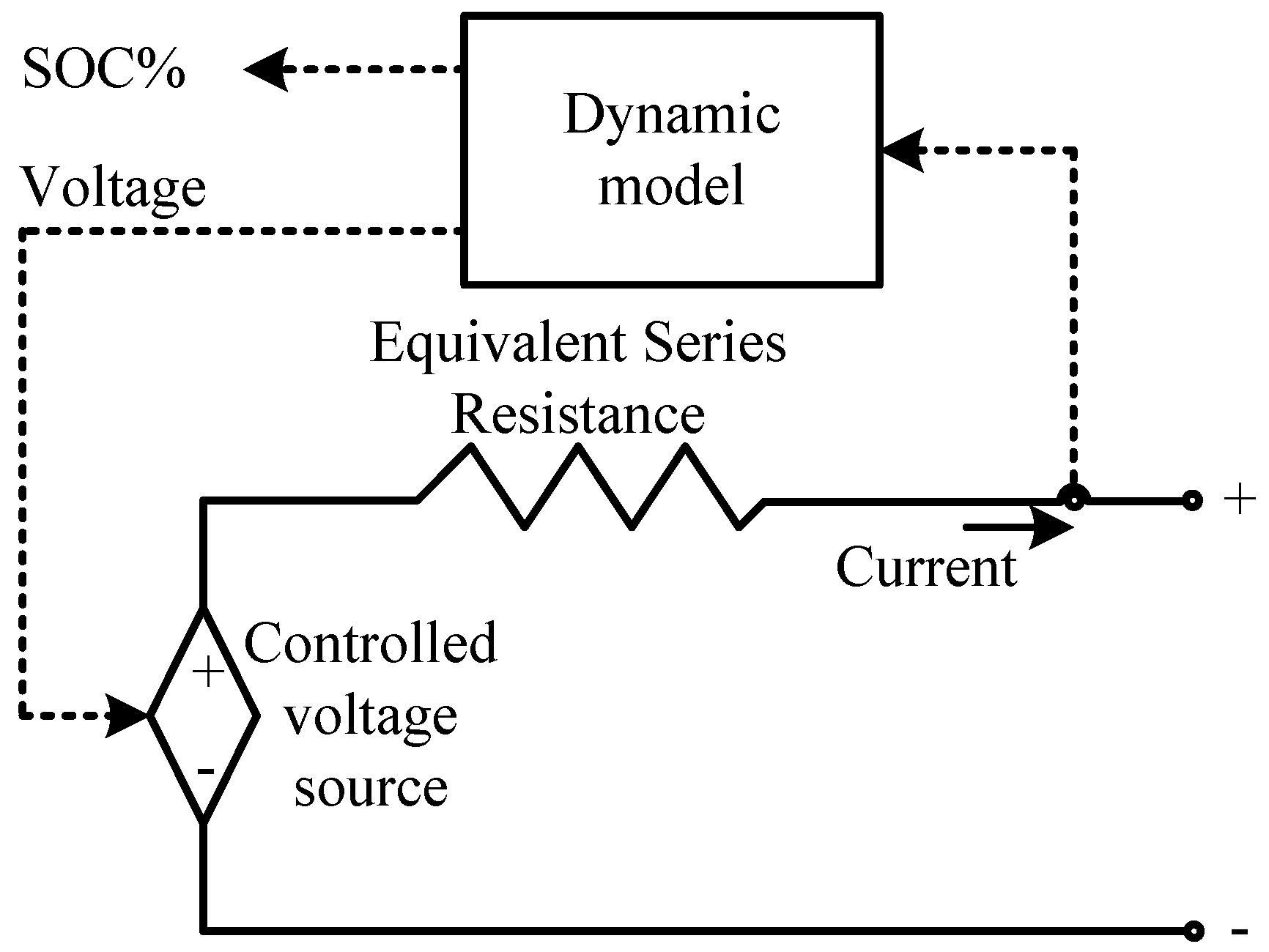
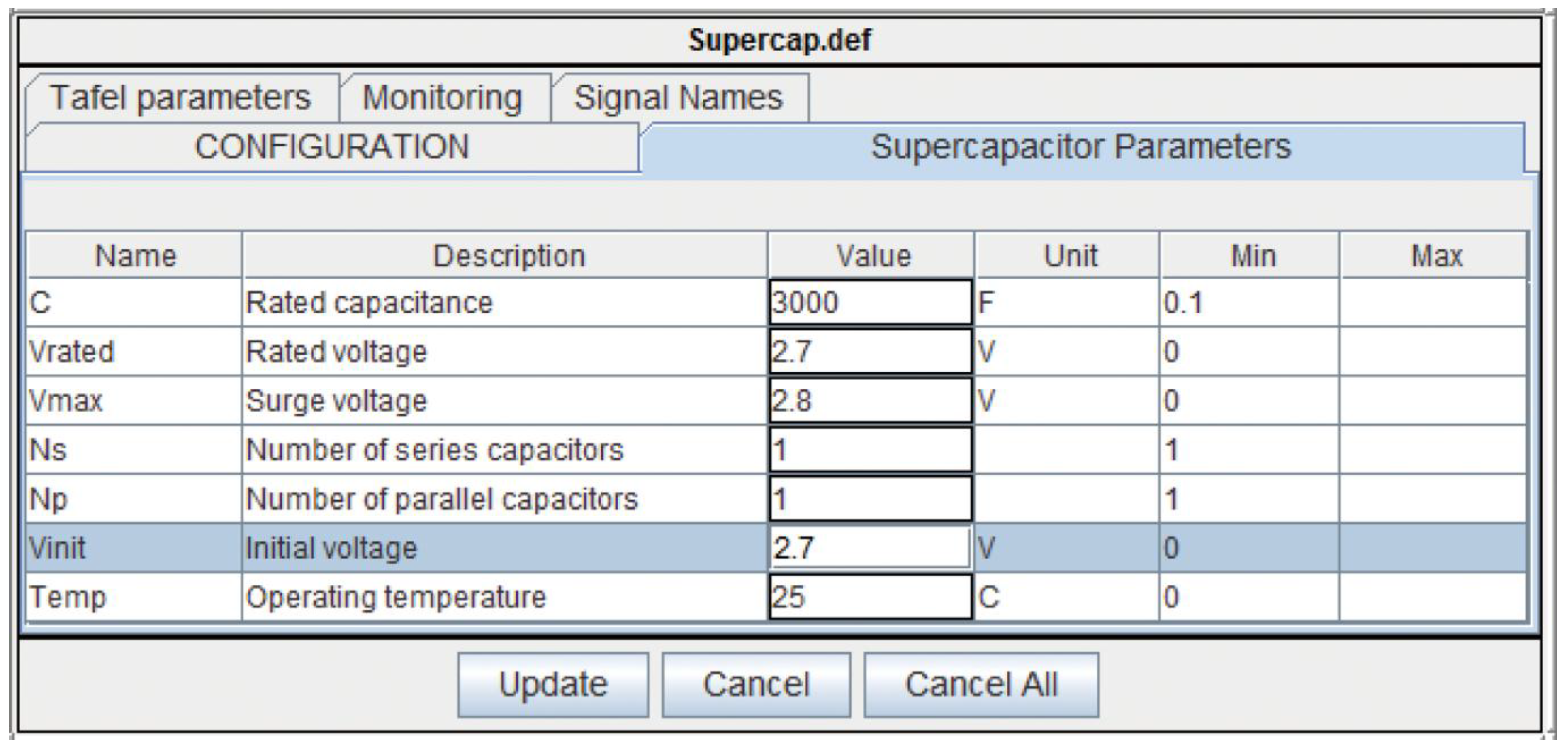
2.1. Development of Electric Double-Layer Capacitor Simulation Model in RSCAD


- Nc number of layers of electrodes;
- Ns number of series EDLC cells;
- Np number of parallel EDLC cells;
- Q electric charge (C);
- r molecular radius (m);
- ε permittivity of material;
- S interfacial area between electrodes and electrolyte (m2);
- R ideal gas constant;
- T operating temperature (F);
- α charge transfer coefficient;
- c molar concentration (mol·m−3);
- i0 exchange current density;
- F faraday constant;
- Vmax surge voltage (V);
- ΔV over-potential (V).

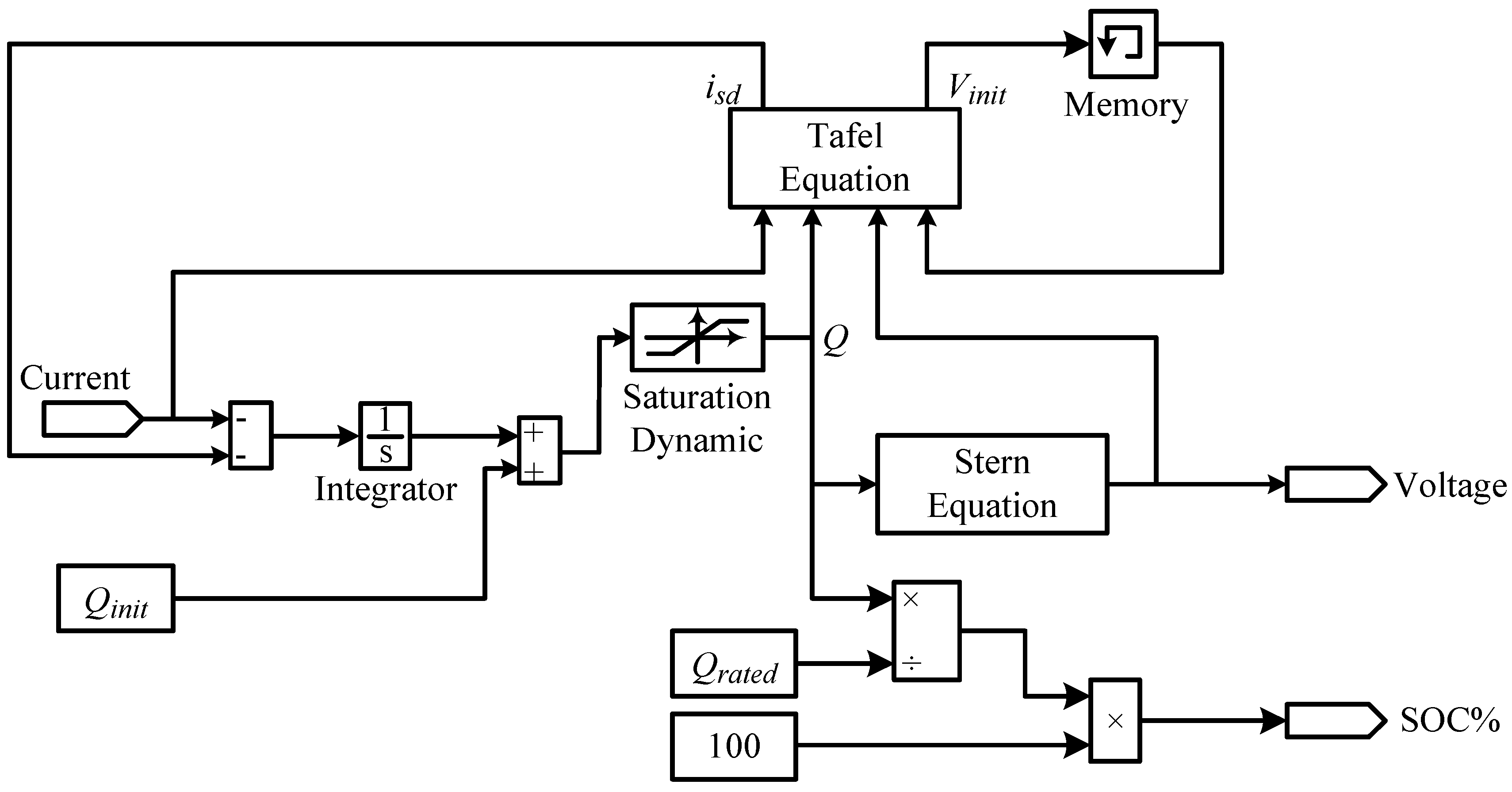
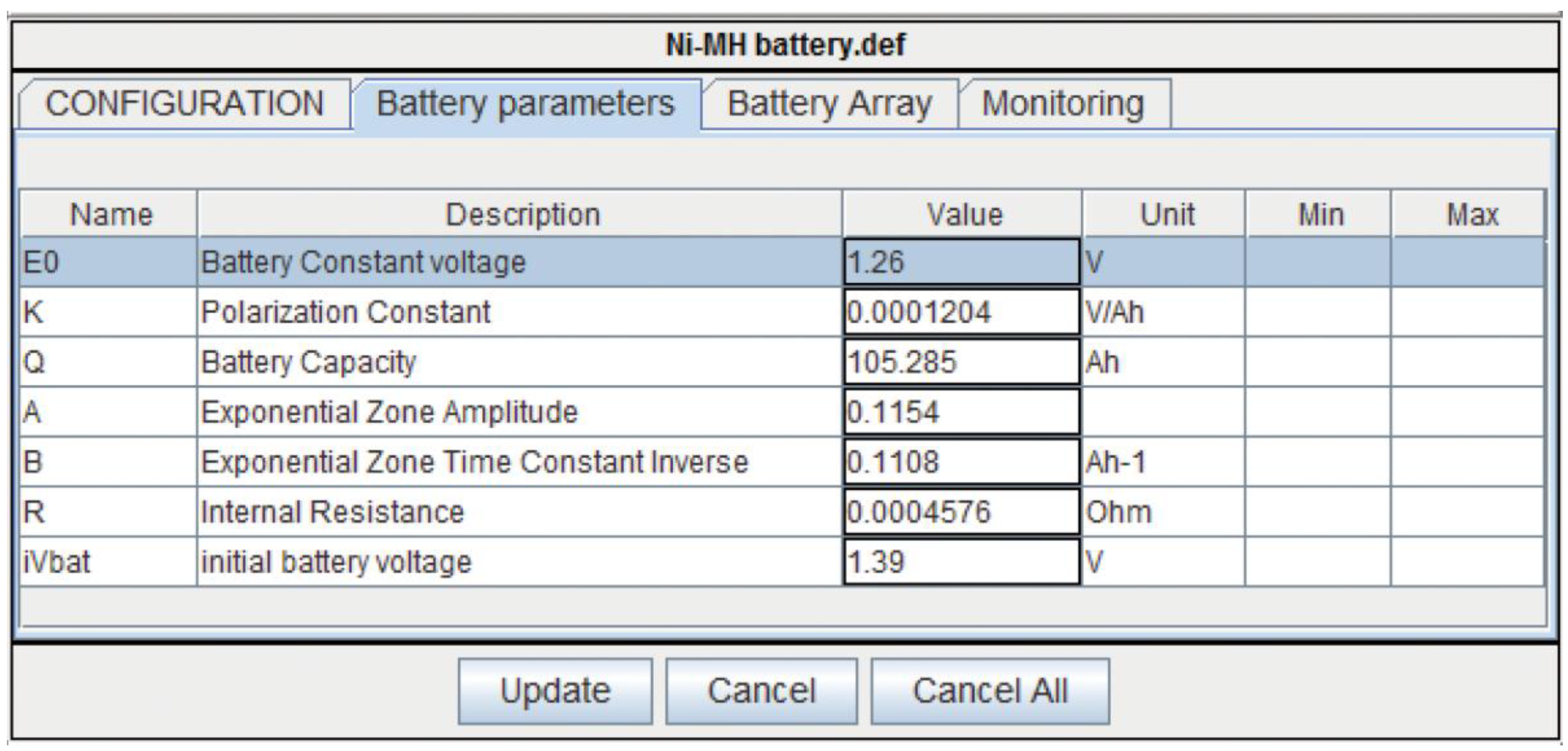
2.2. Development of Ni-MH Battery Simulation Model in RSCAD
- Vbatt battery voltage (V);
- E0 battery constant voltage (V);
- K polarization constant (V/A·h) or polarization resistance (Ω);
- Q battery capacity (A·h);
- it actual battery charge (A·h);
- A exponential zone amplitude (V);
- B exponential zone time constant inverse (A·h)−1;
- R internal resistance (Ω);
- i battery current (A);
- i* filtered current (A).

3. Real-Time Wavelet-Based Energy Management Algorithm
3.1. Data Processing and Discrete Wavelet Transform Procedure
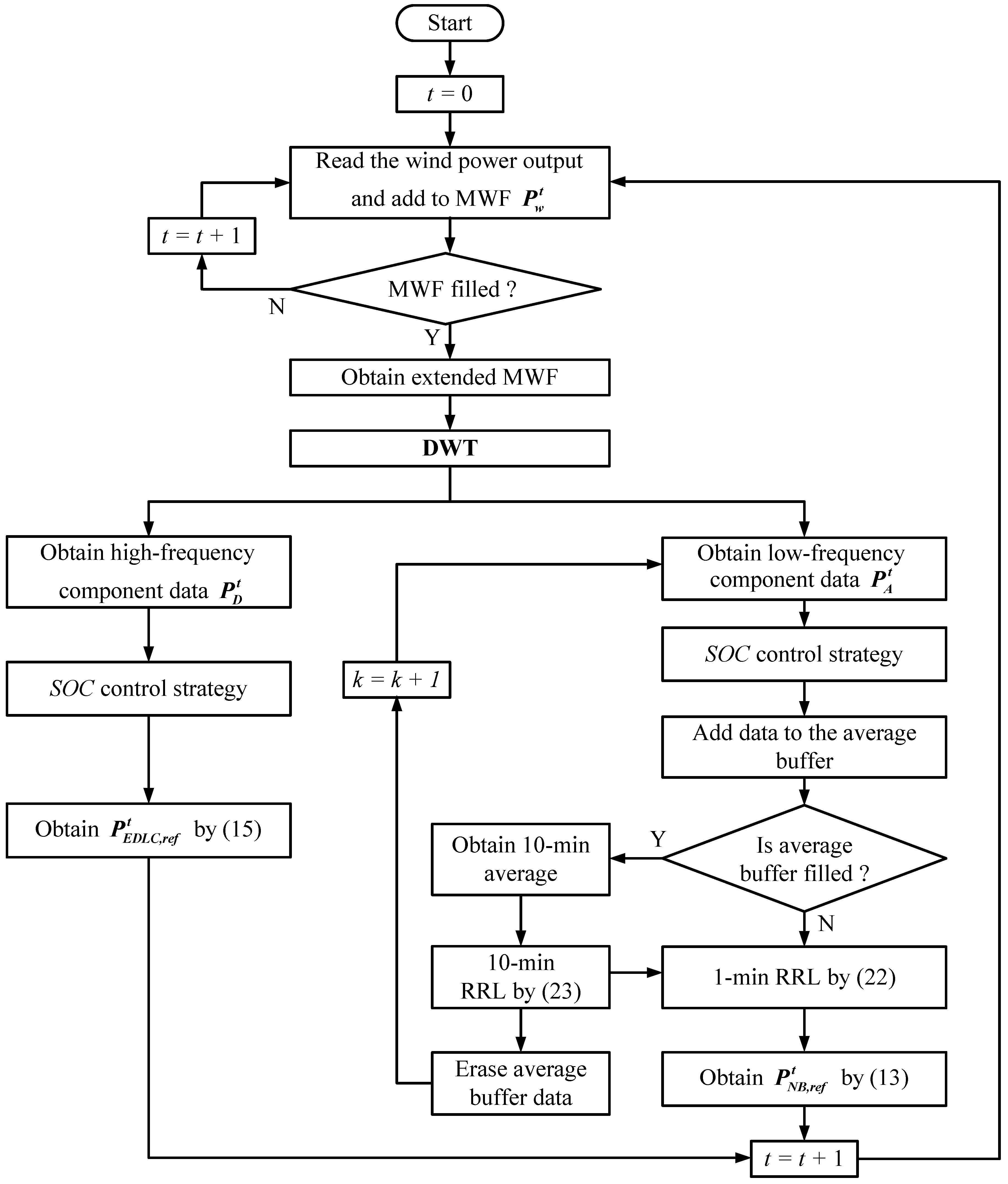
- power output of the wind-HESS system at time t;
- power output of the wind turbine at time t;
- power charged into NB at time t;
- power charged into EDLC at time t.
3.2. State-of-Charge Control Strategies
3.2.1. State-of-Charge Control Strategy of the Electric Double-Layer Capacitor

| EDLC SOC level | Tuning constant (αEDLC) | Battery SOC level | Tuning constant (αNB) |
|---|---|---|---|
| 85% ≤ SOCEDLC | −0.07 | 75% ≤ SOCNB | 1.25 |
| 80% ≤ SOCEDLC < 85% | −0.03 | 70% ≤ SOCNB < 75% | 1.15 |
| 75% ≤ SOCEDLC < 80% | −0.01 | 60% ≤ SOCNB < 70% | 1.05 |
| 45% ≤ SOCEDLC < 75% | 0.01 | 40% ≤ SOCNB < 60% | 1.0 |
| 40% ≤ SOCEDLC < 45% | 0.03 | 35% ≤ SOCNB < 40% | 0.85 |
| 35% ≤ SOCEDLC < 40% | 0.05 | 30% ≤ SOCNB < 35% | 0.75 |
| SOCEDLC < 35% | 0.09 | SOCNB < 30% | 0.65 |
3.2.2. State-of-Charge Control Strategy of the Ni-MH Battery
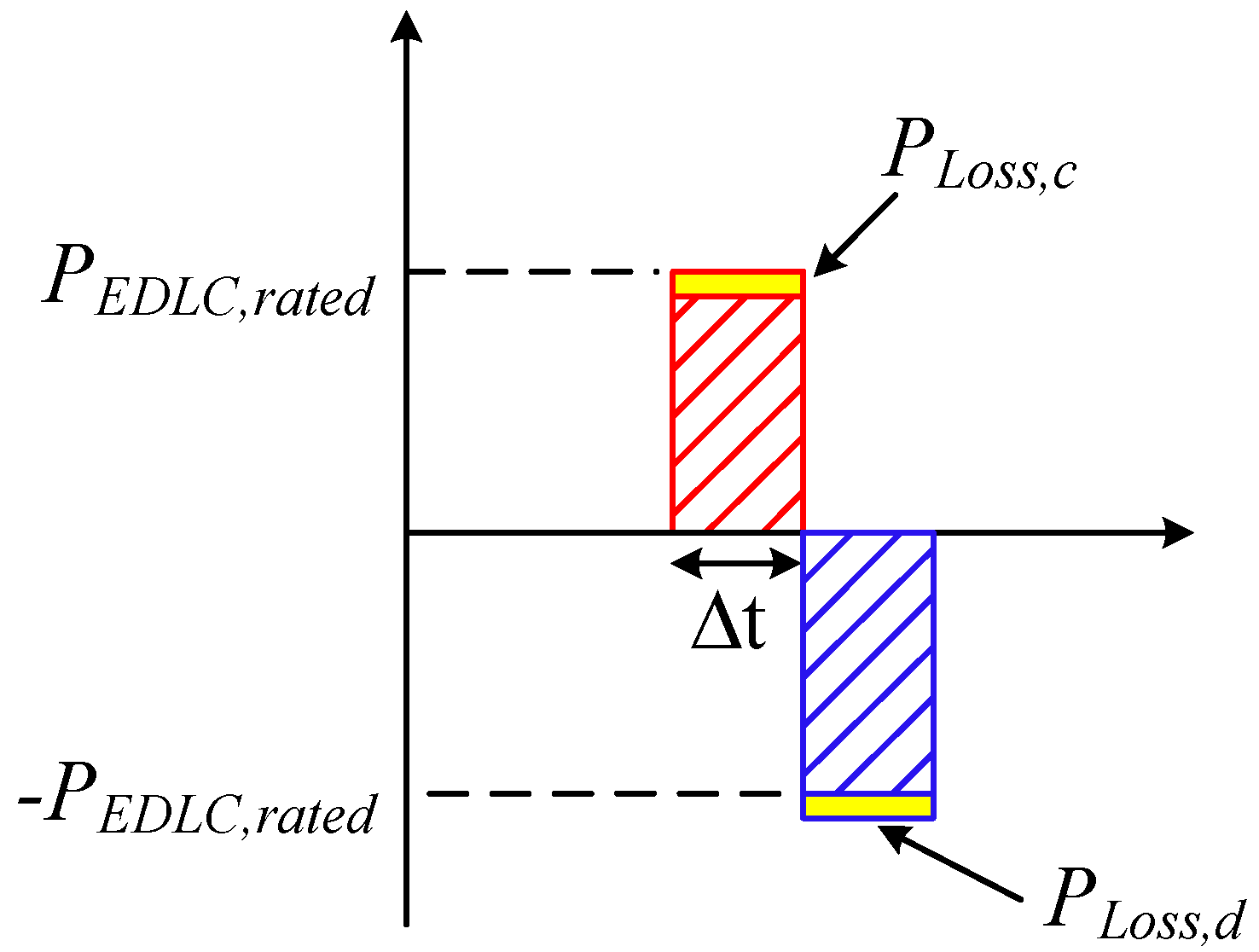
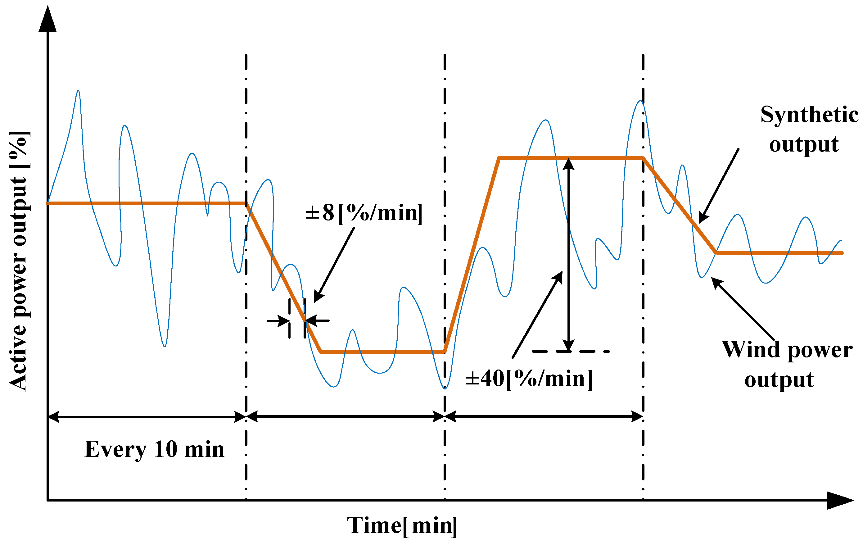
3.3. Ramp Rate Limitation Requirement
4. Simulation Studies
4.1. Configuration of the Test System

| Component | Parameter | Value |
|---|---|---|
| Wind turbine | Pwt,rated | 1.65 MW |
| NB | PNB,rated | 1.0 MW |
| ENB,rated | 0.305 MW·h | |
| EDLC | PEDLC,rated | 0.66 MW |
| EEDLC,rated | 0.022 MW·h |
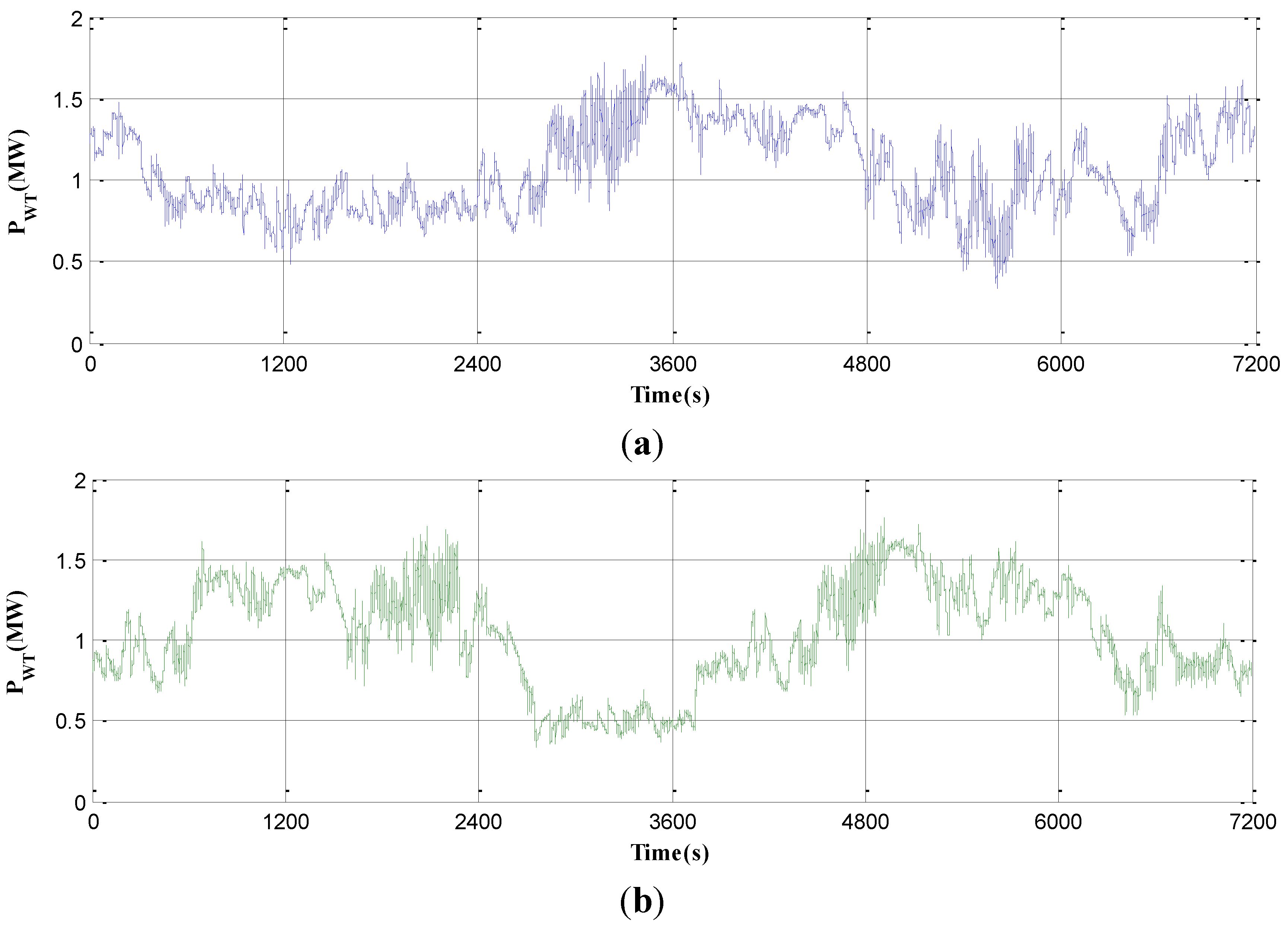
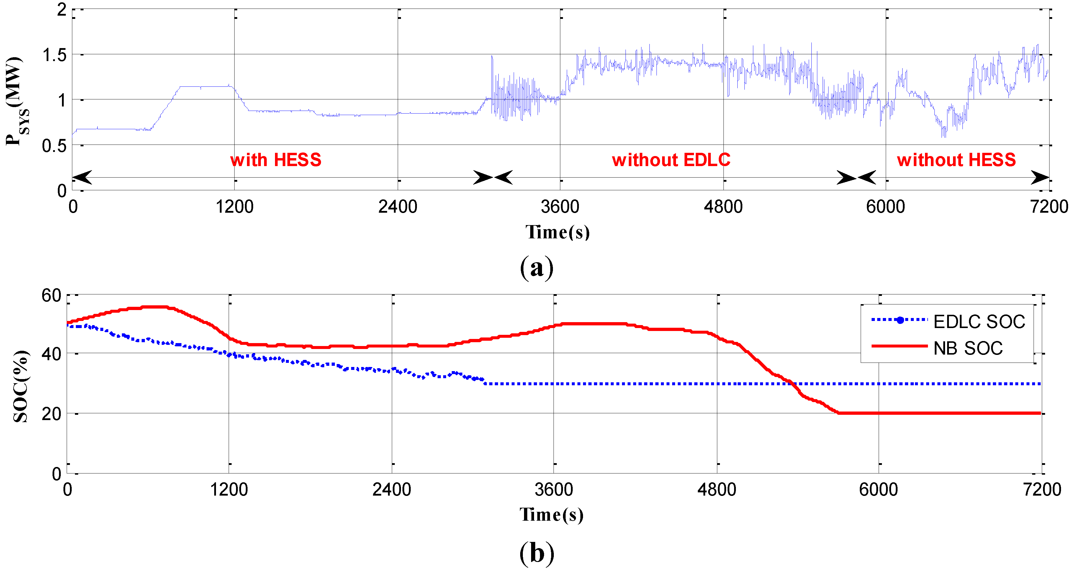
4.2. Case 1: Without State-of-Charge Control Strategy

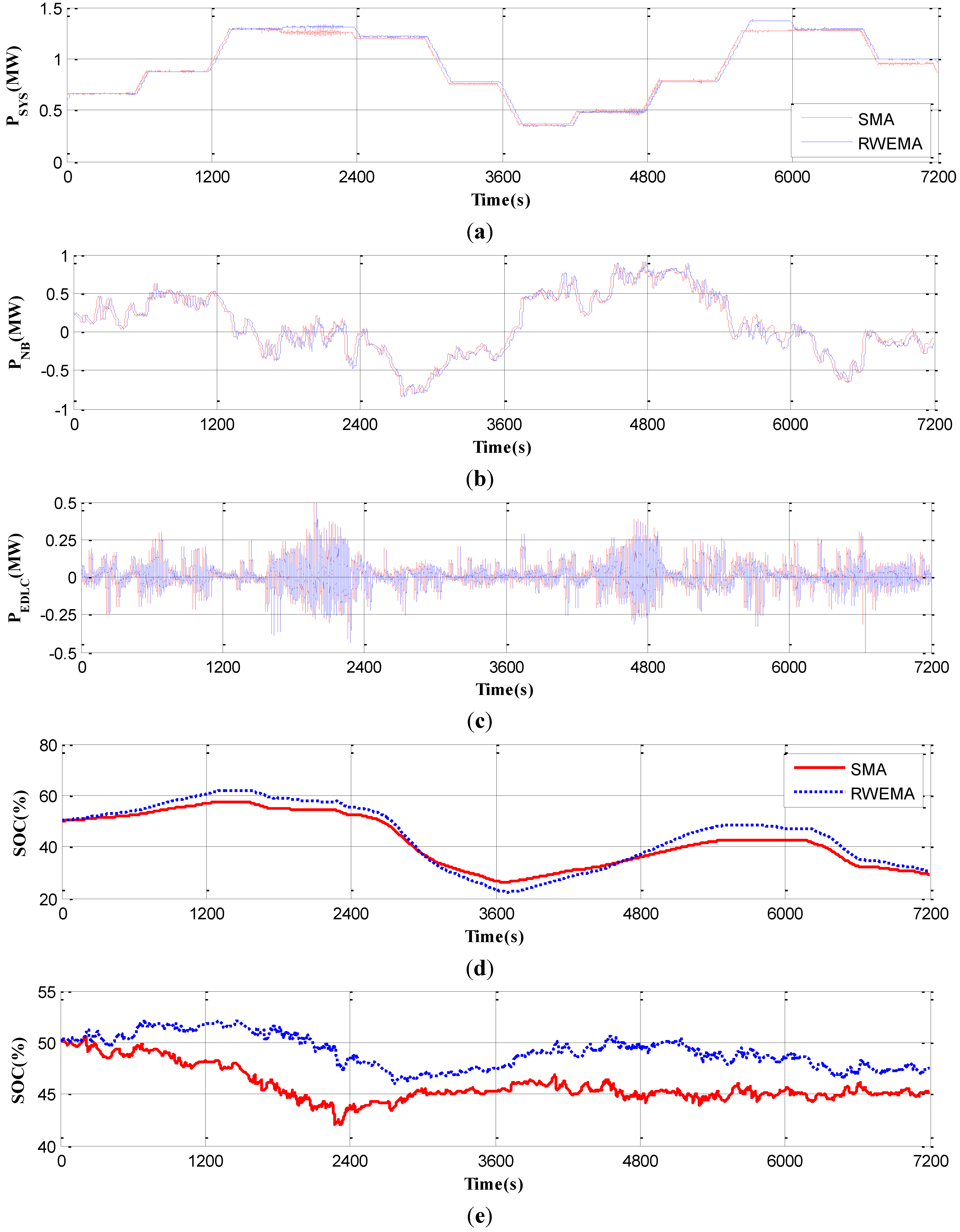
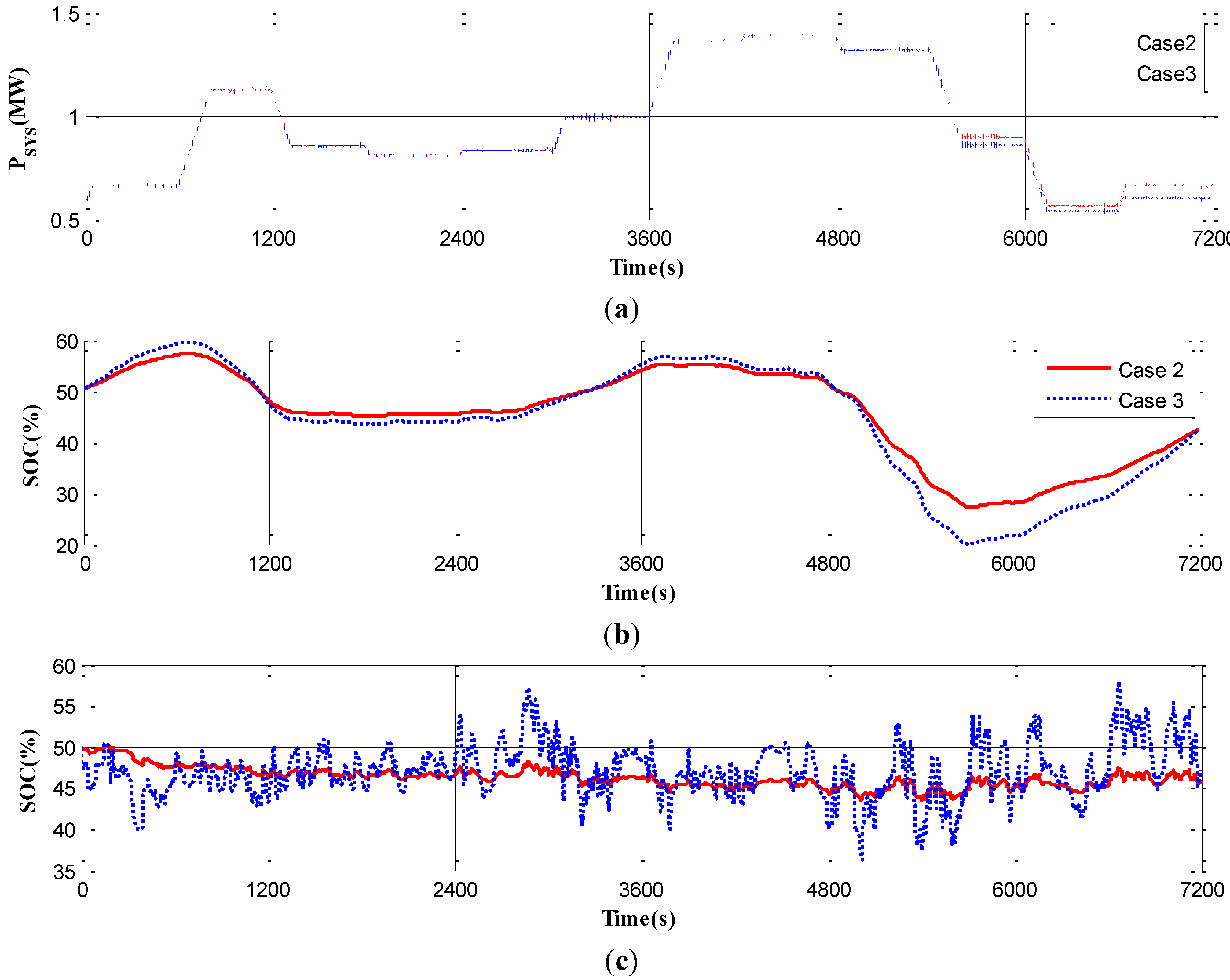
4.3. Case 2: With State-of-Charge Control Strategy and Comparison with Simple Moving Average
- (a)
- Maximum Absolute Value of NB Power Output (): since the cost of the inverter is proportional to the power rating, smaller implies a lower installation cost.
- (b)
- Battery health index (BHI): defined in Equation (24), refers to the degree to which the SOC values deviate from the desired level, typically chosen to be 50%. A smaller BHI indicates more effective usage of the storage device within the safe operating limits [14]:
- (c)
- Average power loss of energy storage ( ) and average system output ( ): the losses in the NB and EDLC during the charge/discharge process and the losses in the inverter will affect the total system output. The average system output is closely related to the revenue of the wind power system operator. The average power loss of the NB and EDLC is defined as Equation (25), where T = 7200 in this study:
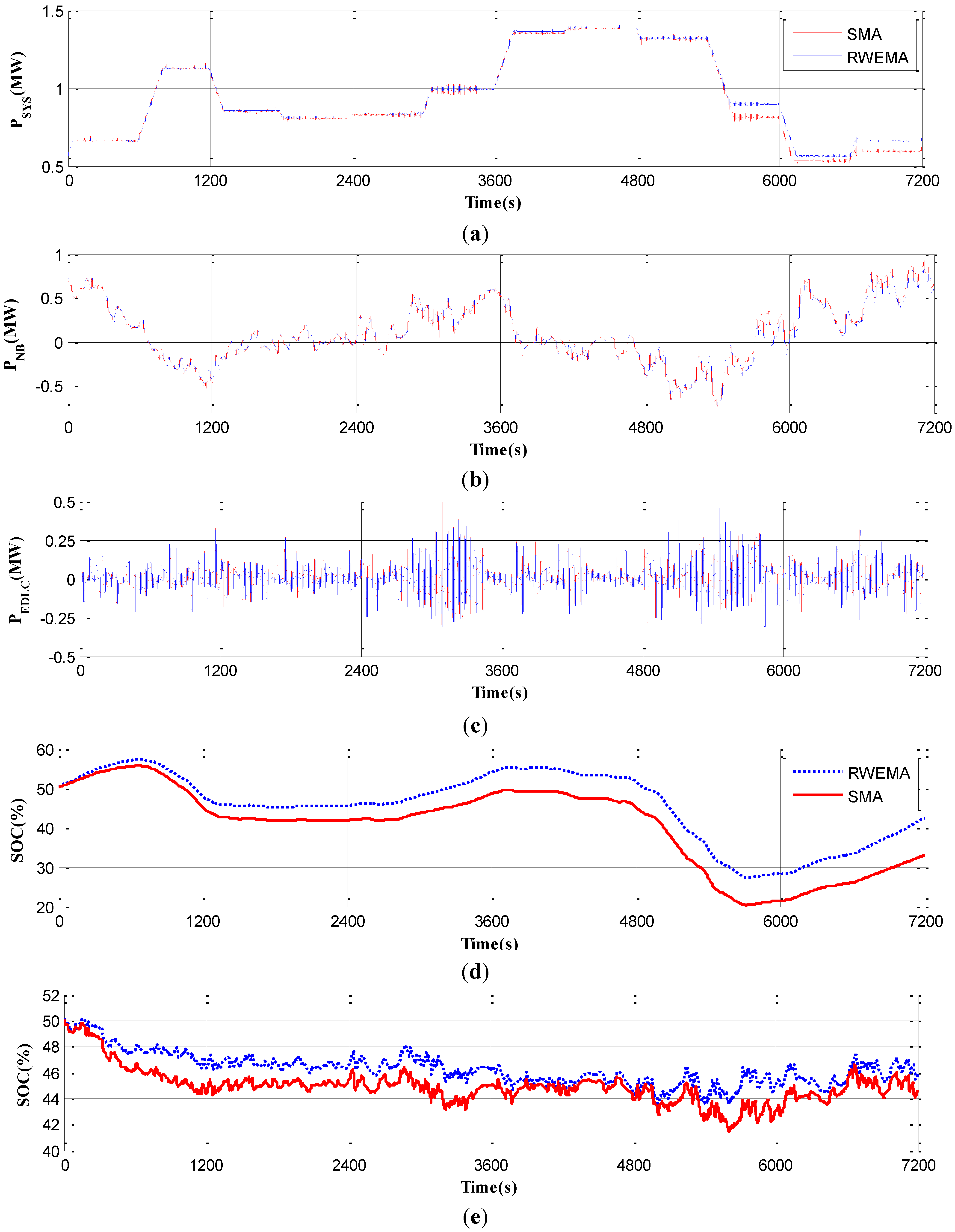
| Case | Methods | BHI | ||||
| Case 2: Wind Pattern 1 | SMA | 0.924 | 13.94 | 137.57 | 14.52 | 0.938 |
| RWEMA | 0.852 | 9.87 | 111.89 | 8.69 | 0.955 | |
| Case 2: Wind Pattern 2 | SMA | 0.912 | 13.25 | 121.51 | 17.09 | 0.929 |
| RWEMA | 0.910 | 12.63 | 112.78 | 10.35 | 0.943 | |
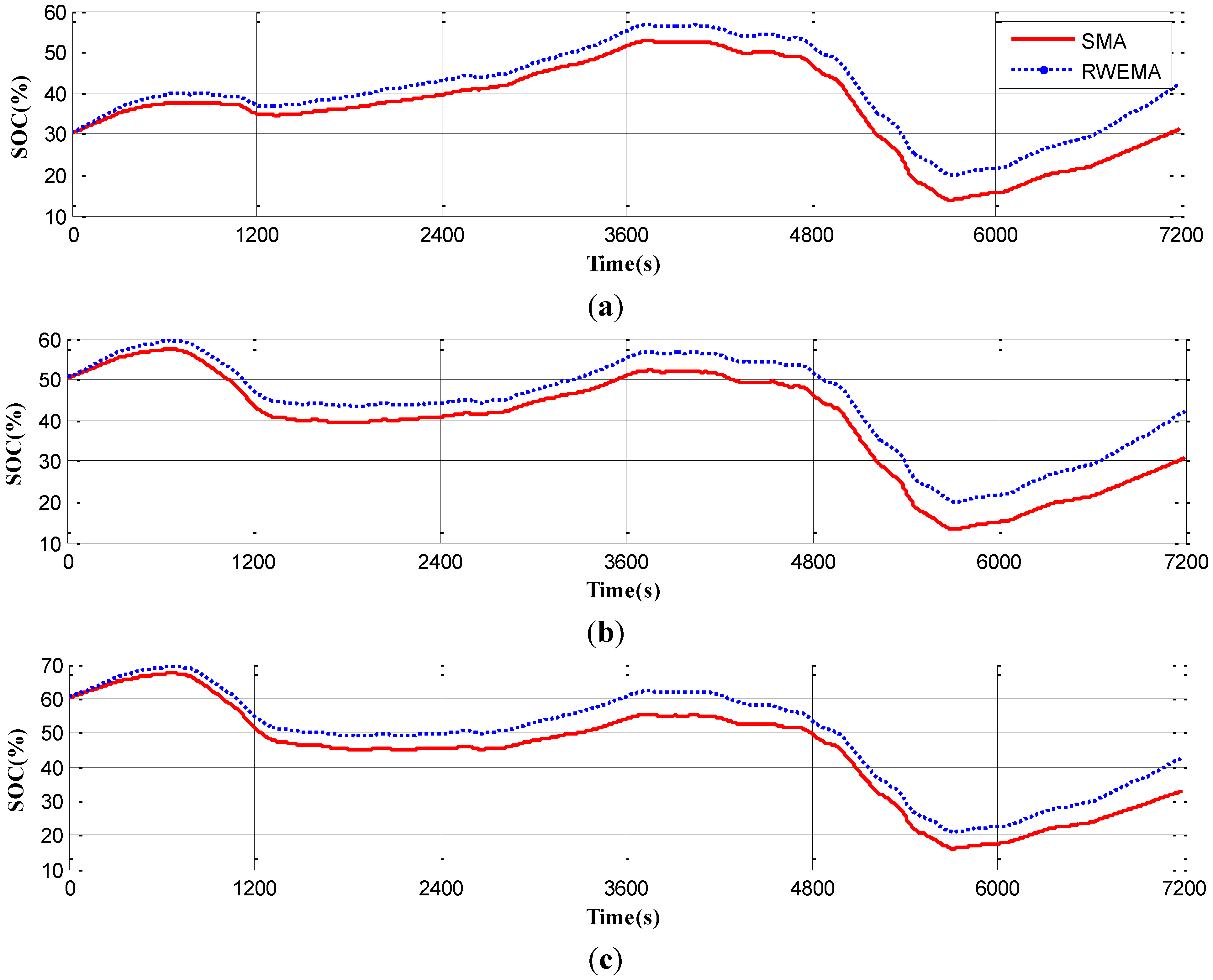
| Case 3: SOC0 = 30% | SMA | 0.919 | 17.79 | 165.82 | 15.35 | 0.881 |
| RWEMA | 0.912 | 14.08 | 135.01 | 9.91 | 0.905 | |
| Case 3: SOC0 = 50% | SMA | 0.921 | 16.72 | 144.31 | 15.39 | 0.926 |
| RWEMA | 0.913 | 12.76 | 118.37 | 9.95 | 0.944 | |
| Case 3: SOC0 = 60% | SMA | 0.920 | 15.77 | 135.92 | 15.33 | 0.944 |
| RWEMA | 0.913 | 13.95 | 114.61 | 9.95 | 0.959 |

4.4. Case 3: Reduced Hybrid Energy Storage System Capacity

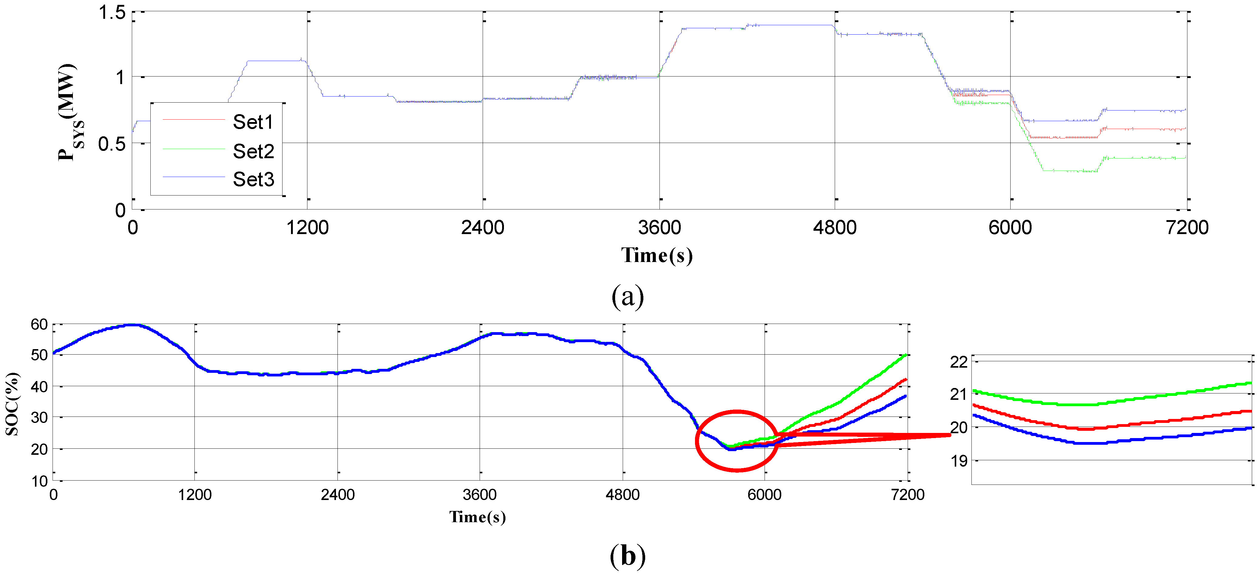
4.5. Case 4: Effect of Tuning Constant
| Battery SOC Level | Tuning constant (αNB) | ||
|---|---|---|---|
| Set 1 | Set 2 | Set 3 | |
| 75% ≤ SOCNB | 1.25 | 1.55 | 1.10 |
| 70% ≤ SOCNB < 75% | 1.15 | 1.35 | 1.05 |
| 60% ≤ SOCNB < 70% | 1.05 | 1.15 | 1.00 |
| 40% ≤ SOCNB < 60% | 1.00 | 1.00 | 1.00 |
| 35% ≤ SOCNB < 40% | 0.85 | 0.75 | 0.90 |
| 30% ≤ SOCNB < 35% | 0.75 | 0.55 | 0.85 |
| SOCNB < 30% | 0.65 | 0.35 | 0.80 |

| Tuning constant set | BHI | |||
| Set 1 | 0.913 | 12.76 | 118.37 | 0.944 |
| Set 2 | 0.997 | 11.75 | 147.29 | 0.906 |
| Set 3 | 0.799 | 13.51 | 102.04 | 0.967 |
5. Conclusions
Acknowledgments
Author Contributions
Conflicts of Interest
References
- Fox, B. Introduction. In Wind Power Integration: Connection and System Operational Aspects; The Institution of Engineering and Technology (IET): London, UK, 2007; pp. 14–18. [Google Scholar]
- Zhang, J.; Cheng, M.; Chen, Z.; Fu, X. Pitch angle control for variable speed wind turbines. In Proceedings of the Third International Conference on Electric Utility Deregulation and Restructuring and Power Technologies, DRPT 2008, Nanjing, China, 6–9 April 2008; pp. 2691–2696.
- Abedini, A.; Nasiri, A. Output power smoothing for wind turbine permanent magnet synchronous generators using rotor inertia. Electr. Power Compon. Syst. 2008, 37, 1–19. [Google Scholar]
- Barton, J.P.; Infield, D.G. Energy storage and its use with intermittent renewable energy. IEEE Trans. Energy Convers. 2004, 19, 441–448. [Google Scholar] [CrossRef]
- Abbey, C.; Joos, G. Supercapacitor energy storage for wind energy applications. IEEE Trans. Ind. Appl. 2007, 43, 769–776. [Google Scholar] [CrossRef]
- Ushiwata, K.; Shishido, S.; Takahashi, R.; Murata, T.; Tamura, J. Smoothing control of wind generator output fluctuation by using electric double layer capacitor. In Proceedings of the International Conference on Electrical Machines and Systems (ICEMS), Seoul, Korea, 8–11 October 2007; pp. 308–313.
- Tanabe, T.; Sato, T.; Tanikawa, R.; Aoki, I.; Funabashi, T.; Yokoyama, R. Generation scheduling for wind power generation by storage battery system and meteorological forecast. In Proceedings of the 2008 IEEE Power and Energy Society General Meeting—Conversion and Delivery of Electrical Energy in the 21st Century, Pittsburgh, PA, USA, 20–24 July 2008; pp. 1–7.
- Sheikh, M.R.I.; Muyeen, S.M.; Takahashi, R.; Murata, T.; Tamura, J. Minimization of fluctuations of output power and terminal voltage of wind generator by using STATCOM/SMES. In Proceedings of the 2009 IEEE Bucharest PowerTech, Bucharest, Romania, 28 June–2 July 2009; pp. 1–6.
- Yoshimoto, K.; Nanahara, T.; Koshimizu, G. New control method for regulating state-of-charge of a battery in hybrid wind power/battery energy storage system. In Proceedings of the 2006 IEEE PES Power Systems Conference and Exposition, PSCE '06, Atlanta, GA, USA, 29 October–1 November 2006; pp. 1244–1251.
- Li, W.; Joós, G.; Bélanger, J. Real-time simulation of a wind turbine generator coupled with a battery supercapacitor energy storage system. IEEE Trans. Ind. Electron. 2010, 57, 1137–1145. [Google Scholar] [CrossRef]
- Suvire, G.O.; Mercado, P. Active power control of a flywheel energy storage system for wind energy applications. IET Renew. Power Gener. 2012, 6, 9–16. [Google Scholar] [CrossRef]
- Mishra, Y.; Mishra, S.; Li, F. Coordinated tuning of DFIG-based wind turbines and batteries using bacteria foraging technique for maintaining constant grid power output. IEEE Syst. J. 2012, 6, 16–26. [Google Scholar] [CrossRef]
- Li, X.; Li, Y.; Han, X.; Hui, D. Application of fuzzy wavelet transform to smooth wind/PV hybrid power system output with battery energy storage system. Energy Procedia 2011, 12, 994–1001. [Google Scholar] [CrossRef]
- Jiang, Q.; Hong, H. Wavelet-based capacity configuration and coordinated control of hybrid energy storage system for smoothing out wind power fluctuations. IEEE Trans. Power Syst. 2013, 28, 1363–1372. [Google Scholar] [CrossRef]
- Xia, R.; Meng, K.; Qian, F.; Wang, Z.-L. Online wavelet denoising via a moving window. Acta Autom. Sin. 2007, 33, 897–901. [Google Scholar] [CrossRef]
- RTDS Technologies. Power System Simulator Hardware. Available online: http://rtds.com/hardware/hardware.html (accessed on 30 May 2014).
- Omar, N.; Daowd, M.; Hegazy, O.; Bossche, P.V.D.; Coosemans, T.; Mierlo, J.V. Electrical double-layer capacitors in hybrid topologies—Assessment and evaluation of their performance. Energies 2012, 5, 4533–4568. [Google Scholar] [CrossRef]
- Oldham, K.B. A Gouy-Chapman-Stern model of the double layer at a (metal)/(ionic liquid) interface. J. Electroanal. Chem. 2008, 613, 131–138. [Google Scholar] [CrossRef]
- MathWorks. Implement Generic Supercapacitor Model—Simulink. Available online: http://www.mathworks.com/help/physmod/sps/powersys/ref/supercapacitor.html (accessed on 3 June 2014).
- Tremblay, O.; Dessaint, L.-A.; Dekkiche, A.-I. A generic battery model for the dynamic simulation of hybrid electric vehicles. In Proceedings of the IEEE Vehicle Power and Propulsion Conference, VPPC 2007, Arlington, TX, USA, 9–12 September 2007; pp. 284–289.
- Gevorgian, V.; Booth, S. Review of Prepa Technical Requirements for Interconnecting Wind and Solar Generation; National Renewable Energy Laboratory: Golden, CO, USA, 2013. [Google Scholar]
- Fox, B. Operation of power systems. In Wind Power Integration: Connection and System Operational Aspects; The Institution of Engineering and Technology (IET): London, UK, 2007; pp. 160–170. [Google Scholar]
- Chan, F.-P.; Fu, A.-C.; Yu, C. Haar wavelets for efficient similarity search of time-series: With and without time warping. IEEE Trans. Knowl. Data Eng. 2003, 15, 686–705. [Google Scholar] [CrossRef]
- Han, S.; Han, S. Economic feasibility of V2G frequency regulation in consideration of battery wear. Energies 2013, 6, 748–765. [Google Scholar] [CrossRef]
- Peterson, S.B.; Apt, J.; Whitacre, J. Lithium-ion battery cell degradation resulting from realistic vehicle and vehicle-to-grid utilization. J. Power Sources 2010, 195, 2385–2392. [Google Scholar] [CrossRef]
© 2014 by the authors; licensee MDPI, Basel, Switzerland. This article is an open access article distributed under the terms and conditions of the Creative Commons Attribution license (http://creativecommons.org/licenses/by/4.0/).
Share and Cite
Trung, T.T.; Ahn, S.-J.; Choi, J.-H.; Go, S.-I.; Nam, S.-R. Real-Time Wavelet-Based Coordinated Control of Hybrid Energy Storage Systems for Denoising and Flattening Wind Power Output. Energies 2014, 7, 6620-6644. https://doi.org/10.3390/en7106620
Trung TT, Ahn S-J, Choi J-H, Go S-I, Nam S-R. Real-Time Wavelet-Based Coordinated Control of Hybrid Energy Storage Systems for Denoising and Flattening Wind Power Output. Energies. 2014; 7(10):6620-6644. https://doi.org/10.3390/en7106620
Chicago/Turabian StyleTrung, Tran Thai, Seon-Ju Ahn, Joon-Ho Choi, Seok-Il Go, and Soon-Ryul Nam. 2014. "Real-Time Wavelet-Based Coordinated Control of Hybrid Energy Storage Systems for Denoising and Flattening Wind Power Output" Energies 7, no. 10: 6620-6644. https://doi.org/10.3390/en7106620
APA StyleTrung, T. T., Ahn, S.-J., Choi, J.-H., Go, S.-I., & Nam, S.-R. (2014). Real-Time Wavelet-Based Coordinated Control of Hybrid Energy Storage Systems for Denoising and Flattening Wind Power Output. Energies, 7(10), 6620-6644. https://doi.org/10.3390/en7106620