Improved Short-Term Load Forecasting Based on Two-Stage Predictions with Artificial Neural Networks in a Microgrid Environment


Abstract
:1. Introduction
2. Data Description and Methodology Framework
2.1. Load Data
2.2. Methodology Framework
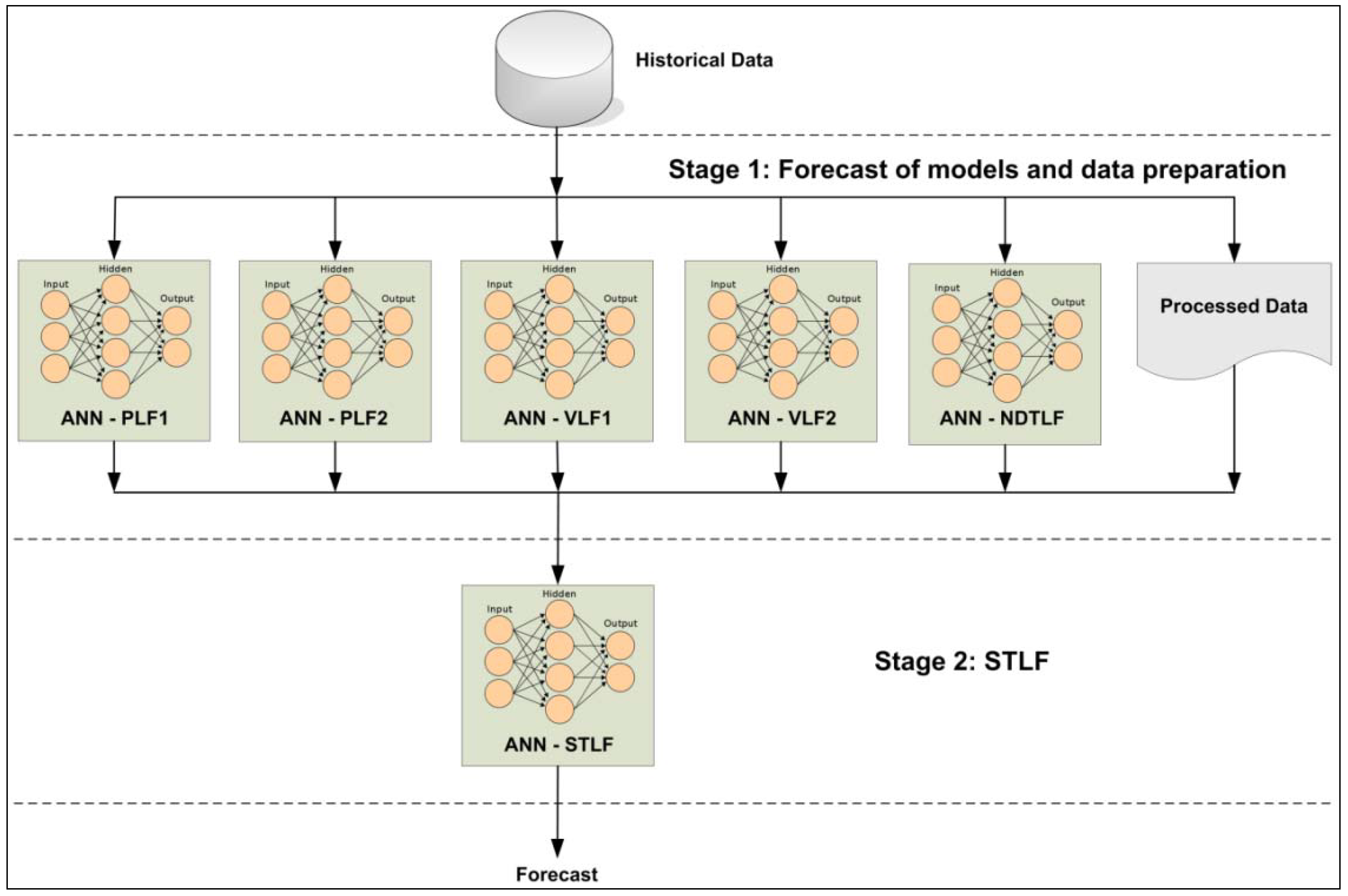
- ANN-PLF1: MLP network, it is responsible for the estimation of the first peak load of the day to forecast. This network will receive the input variables of the database and will present its estimation to the second stage;
- ANN-PLF2: MLP network, it is responsible for the estimation of the second peak load of the day to forecast. This network will receive the input variables of the database and will present its estimation to the second stage;
- ANN-VLF1: MLP network, it is responsible for the estimation of the first valley load of the day to forecast. This network will receive the input variables of the database and will present its estimation to the second stage;
- ANN-VLF2: MLP network, it is responsible for the estimation of the second valley load of the day to forecast. This network will receive the input variables of the database and will present its estimation to the second stage;
- ANN-NDTLF: MLP network, it is responsible for the estimation Next Day’s Total Load (NDTL). This network will receive the input variables of the database and will present its estimation to the second stage;
- Processed data: it is responsible for processing the data from the database expected as input variables by the STLF of the second stage.
3. ANN Structure and Evaluating the Performance of ANN
3.1. ANN–PLFx Structure
- PLi(d−1), PLi(d−2), PLi(d−3), PLi(d−4), PLi(d−5), PLi(d−6), PLi(d−7): peak load of the 7 previous days of the day to forecast; i is 1 or 2;
- PLT(d−1): peak load temperature of the previous day of the day to forecast;
- AvgT(d−1): mean temperature of the previous day to forecast.
- PLid: peak load 1 or 2 of the day to forecast; i is 1 or 2.
3.2. ANN–VLFx Structure
- VLi(d−1), VLi(d−2), VLi(d−3), VLi(d−4), VLi(d−5), VLi(d−6), VLi(d−7): valley load of the 7 previous days of the day to forecast; i is 1 or 2;
- VLT(d−1): valley load temperature of the previous day of the day to forecast;
- AvgT(d−1): mean temperature of the previous day to forecast.
- VLid: valley load 1 or 2 of the day to forecast; i is 1 or 2.
3.3. ANN–NDTLF Structure
- TL(d−1), TL(d−7), TL(d−14), TL(d−21): the total load of a day is clearly linked with the total load of the previous day and total loads of the same day of the week of the three previous weeks, regardless of the type of day, in terms of working/non-working day and day of the week. For this reason, network inputs of the previous day and of the three similar days regarding the day of the week of the three previous weeks, have been selected as total loads;
- W(d−1), W(d−7), W(d−14), W(d−21), Wd: working/non-working day (holiday = 1 and working-day = 2) of the days mentioned in the previous paragraph, as well as the working/non-working day of the day to forecast. The coding is (holiday = 1 and working-day = 2);
- DW(d−1), DW(d−7), DW(d−14), DW(d−21), DWd: day of the week in sine and cosine form, both of the last days mentioned in the first point, as of the day to forecast. The coding is (Sunday = 0, Monday = 1,…, Friday = 5, Saturday = 6);
- SW(d−1), SW(d−7), SW(d−14), SW(d−21), SWd: solar radiation of the last days referred to in the first point, as well as the day to forecast.
- NDTLd.
3.4. ANN–STLF Structure
- L(d−1)1, L(d−1)2, L(d−1)3, L(d−1)24: corresponding to the 24 values of the load curve of the previous day of the day to forecast;
- Day of the week d − 1: this variable is introduced as two, in sines and cosines form, through sin[(2 ⋅ π ⋅ day) / 7 ](d−1) and cos[(2 ⋅ π ⋅ day) / 7 ](d−1), with day values from 0 to 6 (Sunday = 0, Monday = 1, Tuesday = 2, Wednesday = 3, Thursday = 4, Friday = 5, Saturday = 6);
- Month d − 1: this variable is introduced as two, in sines and cosines form, through sin[(2 ⋅ π ⋅ month) / 12 ](d−1) and cos[(2 ⋅ π ⋅ month) / 12 ](d−1), with month values from 1 to 12 (January = 1, February = 2, March = 3,…, December = 12);
- PL1d y PL2d: two maximum values of the load curve of the day to forecast (peak load 1 and peak load 2);
- VL1d y VL2d: two minimum values of the load curve of the day to forecast (valley load 1 and valley load 2);
- NDTLd.
- L(d)1, L(d)2, L(d)3,…,L(d)24: corresponding to the 24 values of the load charge of the day to forecast.
3.5. Evaluating the Performance of ANN
4. Validation Results
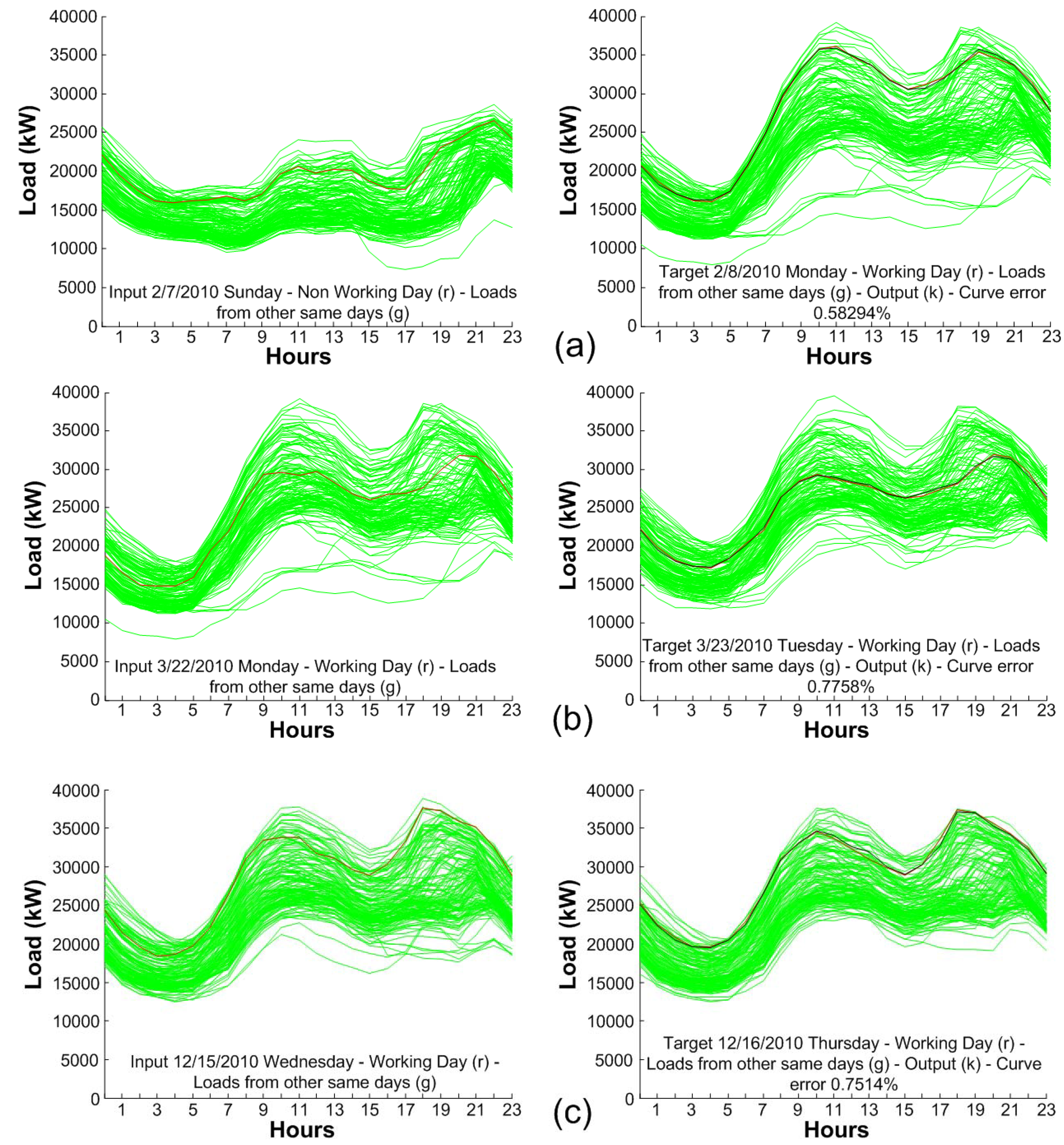
4.1. Results

| Month | MAPE (%) ANN–PLF1 | MAPE (%) ANN–PLF2 | MAPE (%) ANN–VLF1 | MAPE (%) ANN–VLF2 | MAPE (%) ANN–NDTLF |
|---|---|---|---|---|---|
| February | 2.03 | 2.04 | 1.92 | 1.88 | 2.39 |
| March | 2.35 | 2.38 | 2.02 | 1.96 | 2.71 |
| April | 2.30 | 2.15 | 2.12 | 2.05 | 3.26 |
| May | 2.13 | 2.16 | 1.96 | 1.95 | 2.47 |
| June | 2.30 | 2.22 | 2.09 | 2.00 | 4.50 |
| July | 2.04 | 2.08 | 1.87 | 1.90 | 2.63 |
| August | 2.13 | 2.09 | 2.01 | 1.99 | 2.74 |
| September | 2.20 | 2.15 | 2.03 | 2.04 | 1.20 |
| October | 2.84 | 2.67 | 2.22 | 2.10 | 4.86 |
| November | 2.24 | 2.20 | 2.05 | 2.00 | 4.19 |
| December | 2.99 | 2.53 | 2.17 | 2.02 | 3.31 |
| Annual average | 2.32 | 2.24 | 2.04 | 1.99 | 3.11 |

| Variable | Value | Percentage (%) |
|---|---|---|
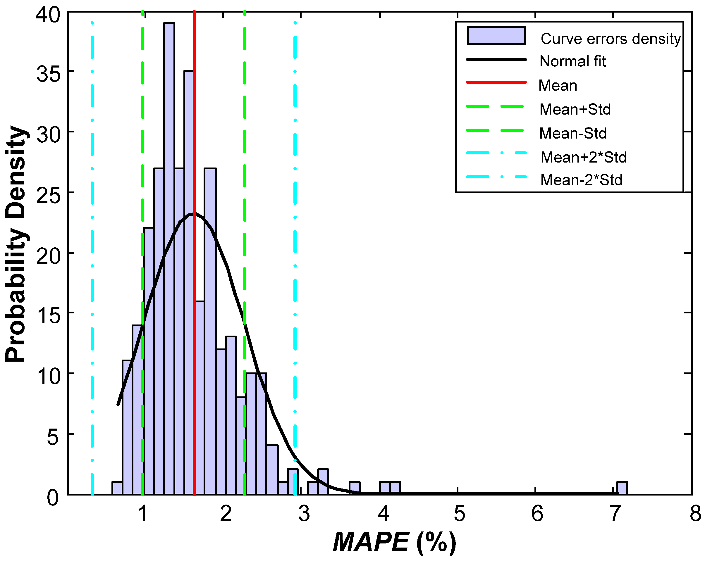
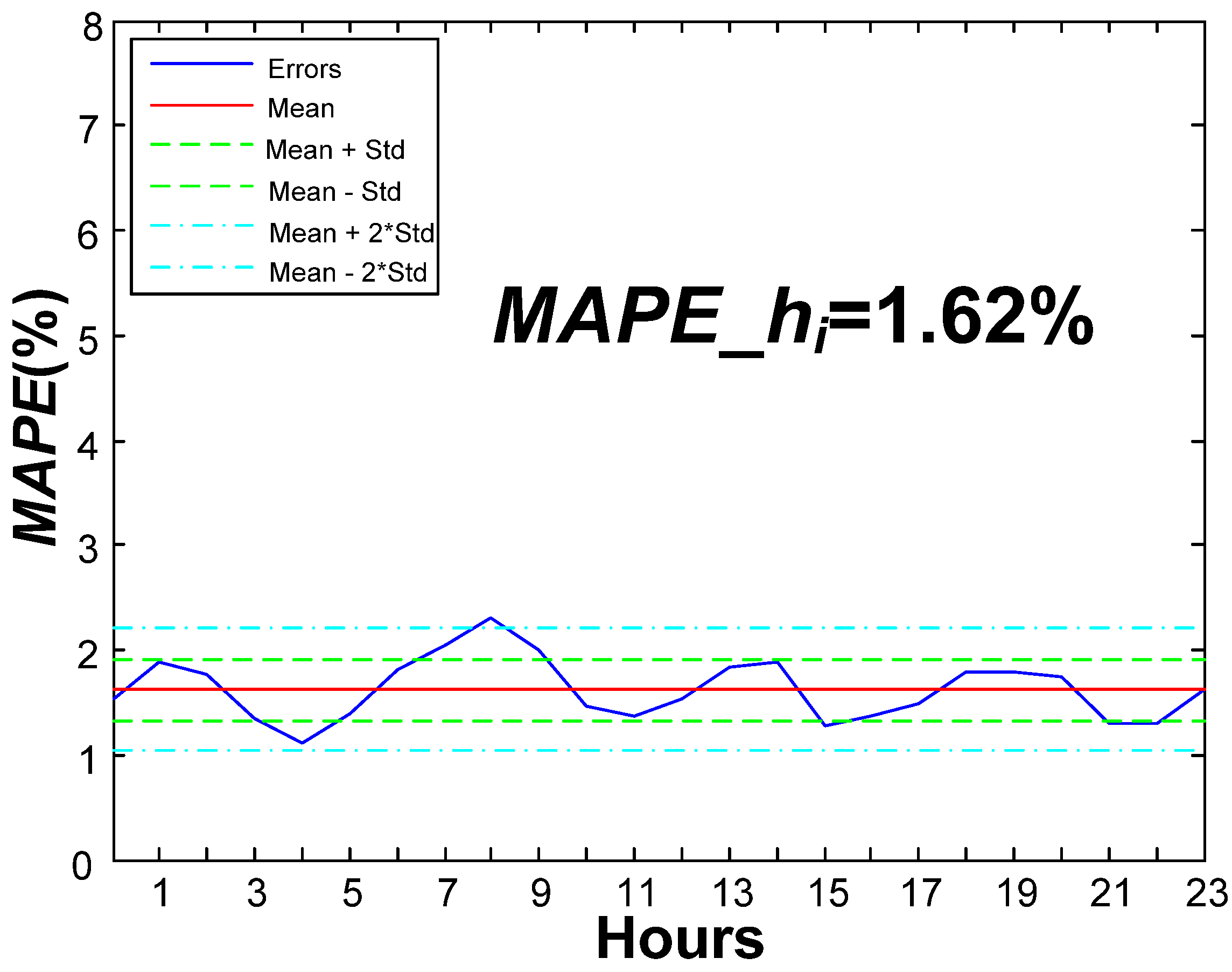
| Mean | 0.162 | 1.62 |
| Standard deviation (Std.) | 0.0065 | 0.65 |
| No. of errors above × 1 Std. | 34 | 11.89 |
| No. of errors between × 1 Std. | 227 | 79.37 |
| No. of errors below × 1 Std. | 25 | 8.74 |
| No. of errors above × 2 Std. | 7 | 2.45 |
| No. of errors between × 2 Std. | 279 | 97.55 |
| No. of errors below × 2 Std. | 0 | 0.00 |
| Variable | Value | Percentage (%) |
|---|---|---|
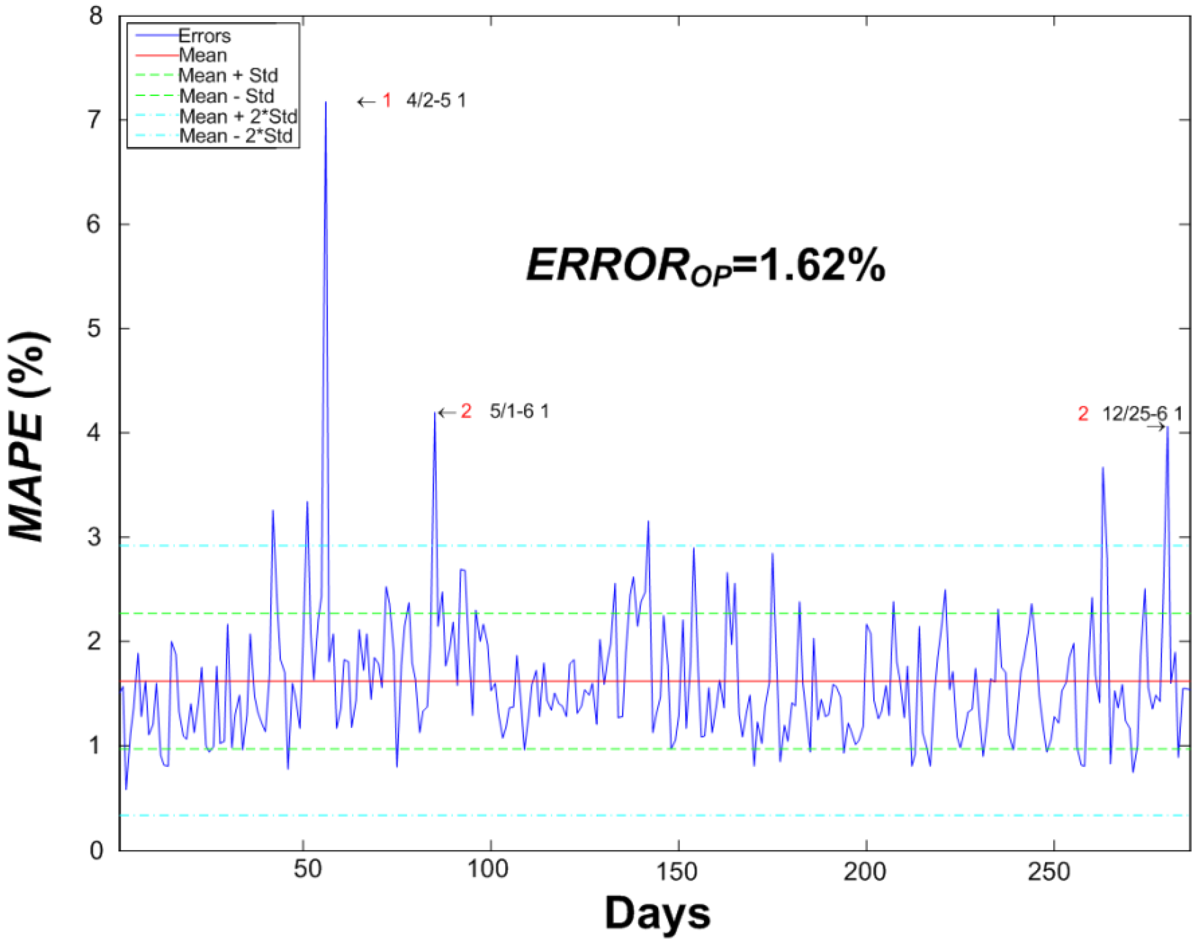
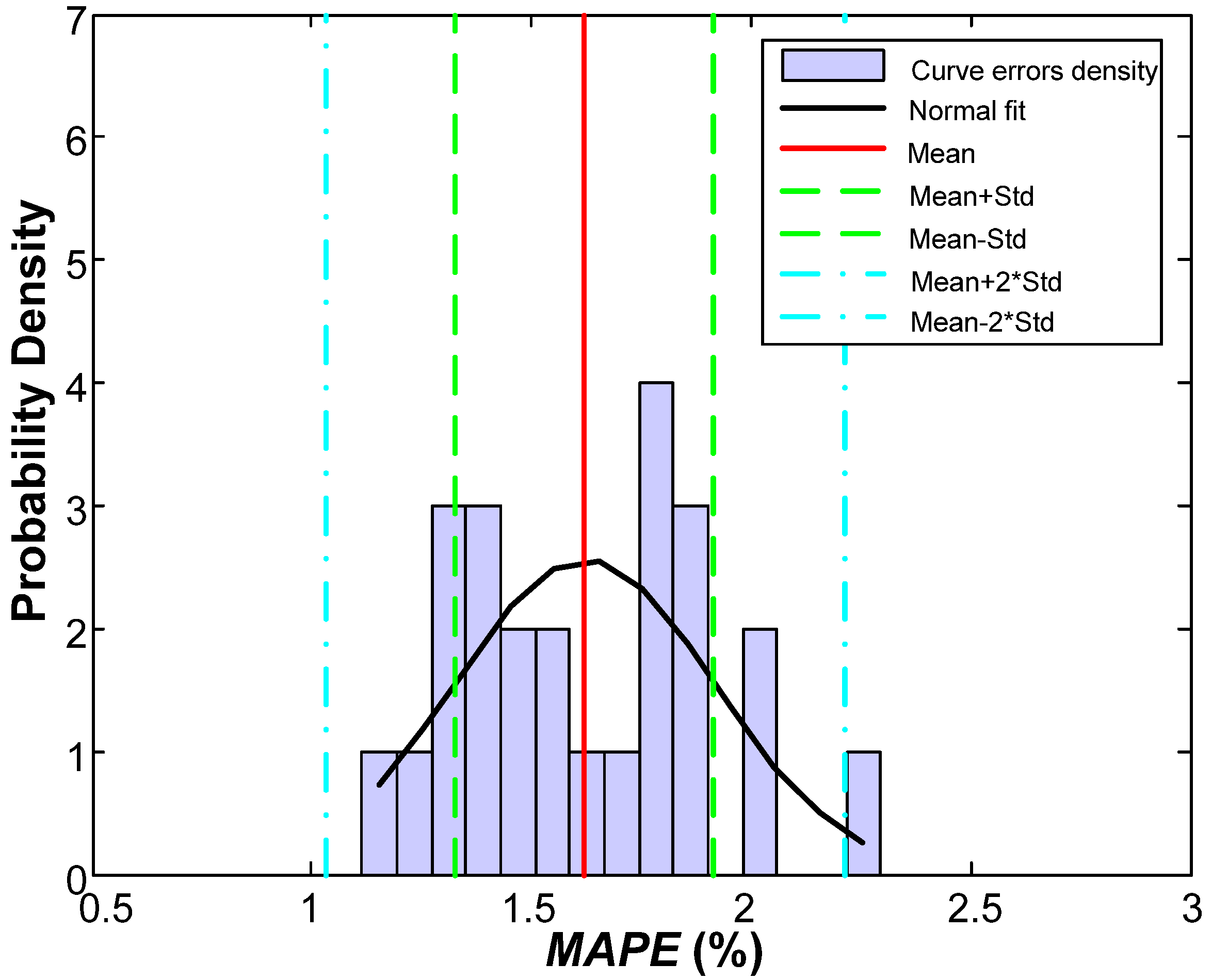
| Mean | 0.0162 | 1.62 |
| Standard deviation (Std.) | 0.0065 | 0.65 |
| No. of errors above × 1 Std. | 3 | 12.50 |
| No. of errors between × 1 Std. | 17 | 70.83 |
| No. of errors below × 1 Std. | 4 | 16.67 |
| No. of errors above × 2 Std. | 1 | 4.17 |
| No. of errors between × 2 Std. | 23 | 95.83 |
| No. of errors below × 2 Std. | 0 | 0.00 |

4.2. Computational Cost
| Forecasts | Learning phase time | Validation phase time |
|---|---|---|
| ANN–PLF1 | 8 min and 17 s | 57 s |
| ANN–PLF2 | 8 min and 25 s | 58 s |
| ANN–VLF1 | 8 min and 02 s | 53 s |
| ANN–VLF1 | 8 min and 05 s | 54 s |
| ANN–NDTLF | 15 min and 45 s | 1 min and 50 s |
| ANN–STLF | 22 min and 15 s | 2 min and 57 s |
5. Result Analysis
5.1. Error Distribution
5.2. Errors per Day of the Week and Month
| Model | Sunday | Monday | Tuesday | Wednesday | Thursday | Friday | Saturday |
|---|---|---|---|---|---|---|---|
| [15] | 2.92 | 2.31 | 2.01 | 1.97 | 2.38 | 2.60 | 2.59 |
| ANN–STLF | 1.89 | 1.57 | 1.34 | 1.41 | 1.56 | 1.64 | 1.91 |
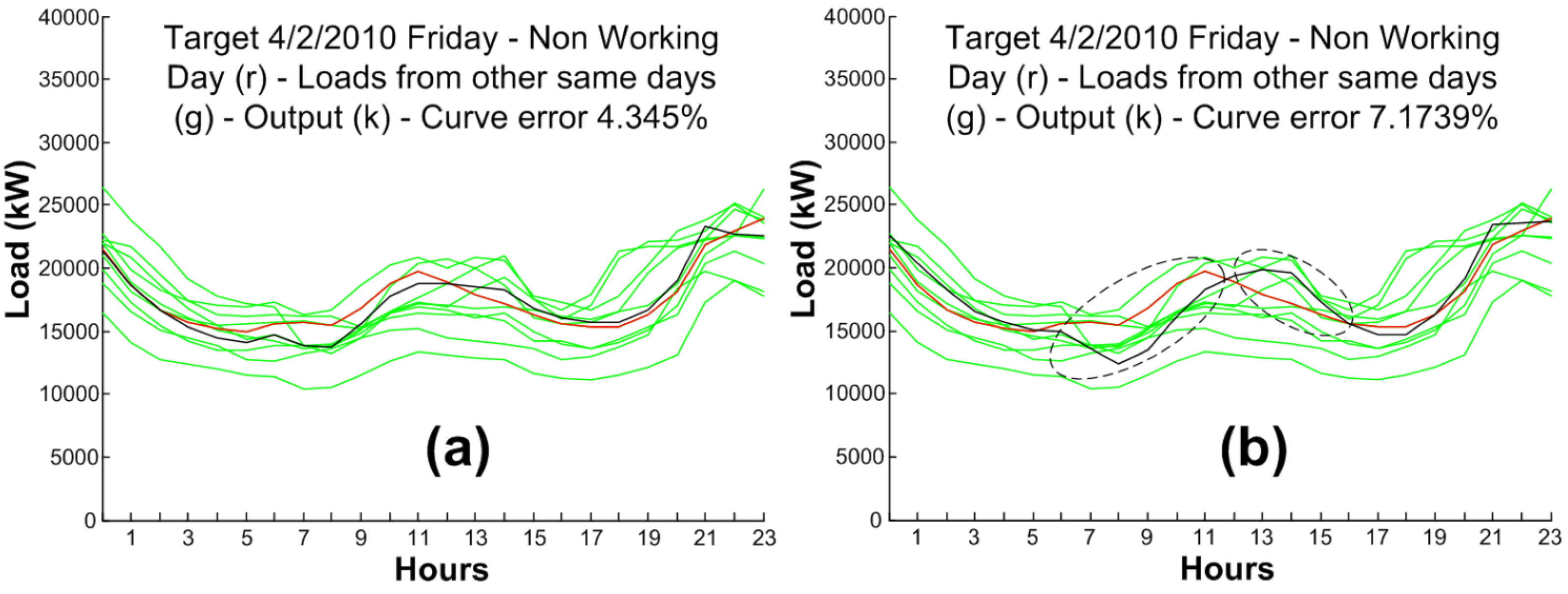
5.3. Error Analysis
| Model | 04/02 | 05/01 | 06/24 | 06/25 | 06/27 | 06/29 | 07/11 | 10/11 | 12/06 | 12/08 | 12/25 | 12/26 | 12/31 |
|---|---|---|---|---|---|---|---|---|---|---|---|---|---|
| [15] | 4.34 | 4.77 | 3.92 | 3.84 | 4.04 | 4.36 | 4.07 | 4.54 | 4.77 | 4.73 | 8.04 | 5.06 | 4.8 |
| ANN–STLF | 7.17 | 4.19 | 2.44 | 2.62 | 2.38 | 3.15 | 2.89 | 2.35 | 1.68 | 3.66 | 4.05 | 1.59 | 1.53 |
6. Conclusions
Acknowledgments
Conflicts of Interest
References
- Simmhan, Y.; Aman, S.; Cao, B.; Giakkaupis, M.; Kumbhare, A.; Zhou, Q.; Paul, D.; Fern, C.; Sharma, A.; Prasanna, V. An Informatics Approach to Demand Response Optimization in Smart Grids; Technical Report for University of Southern California: Los Angeles, CA, USA, 2011. [Google Scholar]
- Brooks, A.; Lu, E.; Reicher, D.; Spirakis, C.; Weihl, B. Demand dispatch. IEEE Power Energy Mag. 2010, 8, 20–29. [Google Scholar] [CrossRef]
- Chan, S.C.; Tsui, K.M.; Wu, H.C.; Hou, Y.; Wu, Y.-C.; Wu, F.F. Load/price forecasting and managing demand response for smart grids. IEEE Signal Process. Mag. 2012, 29, 68–85. [Google Scholar] [CrossRef]
- O’Toole, E.; Clarke, S. Dynamic Forecasting and Adaptation for Demand Optimization in the Smart Grid. In Proceedings of 2012 International Workshop on Software Engineering for the Smart Grid (SE4SG), Zurich, Switzerland, 3 June 2012; pp. 30–33.
- Saini, L.M.; Soni, M.K. Artificial neural network-based peak load forecasting using conjugate gradient methods. IEEE Trans. Power Syst. 2002, 17, 907–912. [Google Scholar] [CrossRef]
- Hyndman, R.J.; Fan, S. Density forecasting for long-term peak electricity demand. IEEE Trans. Power Syst. 2010, 25, 1142–1153. [Google Scholar] [CrossRef]
- McSharry, P.E.; Bowman, S.; Bloemhof, G. Probabilistic forecasts of the magnitude and timing of peak electricity demand. IEEE Trans. Power Syst. 2005, 20, 1166–1172. [Google Scholar] [CrossRef]
- Amin-Naseri, M.R.; Soroush, A.R. Combined use of unsupervised and supervised learning for daily peak load forecasting. Energy Convers. Manag. 2008, 49, 1302–1308. [Google Scholar] [CrossRef]
- Maksimovich, S.M.; Shiljkut, V.M. The peak load forecasting afterwards its intensive reduction. IEEE Power Deliv. 2009, 24, 1552–1559. [Google Scholar] [CrossRef]
- Moazzami, M.; Khodabakhshian, A.; Hooshmand, R. A new hybrid day-ahead peak load forecasting method for Iran’s National Grid. Appl. Energy 2013, 101, 489–501. [Google Scholar] [CrossRef]
- Jain, A.; Satish, B. Integrated Approach for Short-Term Load Forecasting Using SVM and ANN. In Proceedings of IEEE TENCON 2008 Region Conference, Hyderabad, India, 19–21 November 2008; pp. 1–6.
- Amral, N.; King, D.; Ozveren, C.S. Application of Artificial Neural Network for Short Term Load Forecasting. In Proceedings of 43rd International Universities Power Engineering Conference (UPEC), Padova, Italy, 1–4 September 2008; pp. 1–5.
- Lasseter, R.; Akhil, A.; Marnay, C.; Stevens, J.; Dagle, J.; Guttromson, R.; Meliopoulous, A.S.; Yinger, R.; Eto, J. White Paper on Integration of Distributed Energy Resources. The CERTS Microgrid Concept; Consortium for Electric Reliability Technology Solutions (CERTS): Los Angeles, CA, USA, 2002.
- Hernández, L.; Baladrón, C.; Aguiar, J.M.; Carro, B.; Sánchez-Esguevillas, A. Classification and clustering of electricity demand patterns in industrial parks. Energies 2012, 5, 5215–5228. [Google Scholar] [CrossRef]
- Hernández, L.; Baladrón, C.; Aguiar, J.M.; Carro, B.; Sánchez-Esguevillas, A.; Lloret, J. Short-term load forecasting for microgrids based on artificial neural networks. Energies 2013, 6, 1385–1408. [Google Scholar] [CrossRef]
- Drezga, I.; Rahman, S. Phase-Space Short-Term Load Forecasting for Deregulated Electric Power Industry. In Proceedings of the International Joint Conference on Neural Networks, Washington, DC, USA, 10–16 July 1999; Volume 5, pp. 3405–3409.
- Razavi, S.; Tolson, B.A. A new formulation for feedforward neural networks. IEEE Trans. Neural Netw. 2011, 22, 1588–1598. [Google Scholar] [CrossRef] [PubMed]
- Ghomi, M.; Goodarzi, M. Peak Load Forecasting of Electric Utilities for West Province of Iran by Using Neural Network without Weather Information. In Proceedings of 12th International Conference on Computer Modelling and Simulation (UKSim), Cambridge, UK, 24–26 March 2010; pp. 28–32.
- Hernández, L.; Baladrón, C.; Aguiar, J.M.; Carro, B.; Sánchez-Esguevillas, A.; García, P.; Lloret, J. Experimental analysis of the input variables’ relevance to forecast next day’s aggregated electric demand using neural networks. Energies 2013, 6, 2927–2948. [Google Scholar] [CrossRef]
- Hernández, L.; Baladrón, C.; Aguiar, J.M.; Carro, B.; Sánchez-Esguevillas, A.; Lloret, J.; Chinarro, D.; Gómez-Sanz, J.J.; Cook, D. A multi-agent system architecture for smart grid management and forecasting of energy demand in virtual power plants. IEEE Commun. Mag. 2013, 51, 106–113. [Google Scholar] [CrossRef]
© 2013 by the authors; licensee MDPI, Basel, Switzerland. This article is an open access article distributed under the terms and conditions of the Creative Commons Attribution license (http://creativecommons.org/licenses/by/3.0/).
Share and Cite
Hernández, L.; Baladrón, C.; Aguiar, J.M.; Calavia, L.; Carro, B.; Sánchez-Esguevillas, A.; Sanjuán, J.; González, Á.; Lloret, J. Improved Short-Term Load Forecasting Based on Two-Stage Predictions with Artificial Neural Networks in a Microgrid Environment. Energies 2013, 6, 4489-4507. https://doi.org/10.3390/en6094489
Hernández L, Baladrón C, Aguiar JM, Calavia L, Carro B, Sánchez-Esguevillas A, Sanjuán J, González Á, Lloret J. Improved Short-Term Load Forecasting Based on Two-Stage Predictions with Artificial Neural Networks in a Microgrid Environment. Energies. 2013; 6(9):4489-4507. https://doi.org/10.3390/en6094489
Chicago/Turabian StyleHernández, Luis, Carlos Baladrón, Javier M. Aguiar, Lorena Calavia, Belén Carro, Antonio Sánchez-Esguevillas, Javier Sanjuán, Álvaro González, and Jaime Lloret. 2013. "Improved Short-Term Load Forecasting Based on Two-Stage Predictions with Artificial Neural Networks in a Microgrid Environment" Energies 6, no. 9: 4489-4507. https://doi.org/10.3390/en6094489
APA StyleHernández, L., Baladrón, C., Aguiar, J. M., Calavia, L., Carro, B., Sánchez-Esguevillas, A., Sanjuán, J., González, Á., & Lloret, J. (2013). Improved Short-Term Load Forecasting Based on Two-Stage Predictions with Artificial Neural Networks in a Microgrid Environment. Energies, 6(9), 4489-4507. https://doi.org/10.3390/en6094489