1. Introduction
Most people believe that finding a treasure is a fortunate event that promises future happiness. However, Sachs and Warner [
1] and Gylfason [
2] show, puzzlingly, that countries with great natural resources tend to grow slower than countries that have fewer natural resources at their disposal. There is a growing body of literature on this paradox of plenty, recently surveyed by Boyce and Emery [
3]. However, the explicit consideration of various effects of an energy production on an economic growth has lead to more ambiguous results [
4,
5]. So far the paradoxical growth rates and conditions of energy rich countries, has been still one of the issues challenging scholars in the energy economics area [
6,
7].
Over the past several decades, China has made tremendous progress in market integration and infrastructure development [
8]. Market reforms have eased restrictions on the flows of products, labour and capital. The newly built inter-provincial highway system provides better transport links between regions and promotes trade flow. Rapid productivity growth has lowered the price of manufactured goods and led to a soaring demand for energy production, which are supplied by the resource-abundant interior regions. Energy resources serve as an important capital in economic development. In principle, revenues generated from the energy production sector should be good for the economy. Given this situation-increasing market integration, better transport systems and more favourable terms of trade-growth theory predicts a regional convergence. However, in China the heavy energy production seems to not match the rapid regional economic growth.
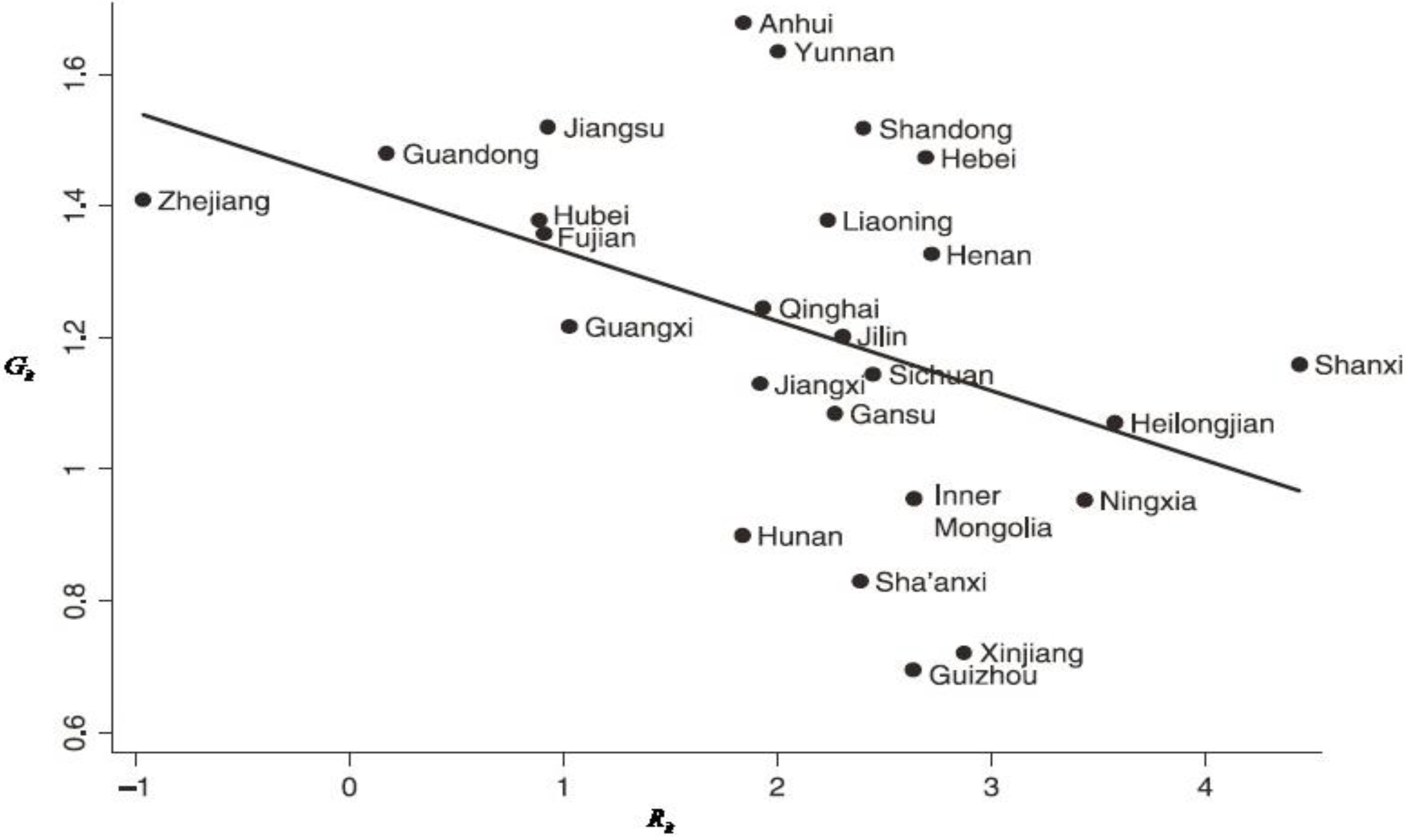
Figure 1 plots
per capita GDP growth [
] from 1985 to 2010 against the energy production intensity (
,
denoted as the ratio of energy production to total GDP for
ith province, in which the energy production is defined as the total standard energy units of coal, oil, natural gas and hydraulic power). The figure shows a negative link between the energy production intensity and average growth rate of
per capita GDP in the following 26 years in China as a whole. Most provinces with a rapid growth, such as Zhejiang Province started as an energy resource-poor, while energy resource-rich provinces, such as Guizhou, Shanxi and Heilongjiang grew more slowly than average. Obviously, given that the resource-rich interior regions are poorer than the resource poor regions, it can be predicted that a convergence should favor more rapid growth in resource-rich regions. Thus, the issues that whether the energy production is a curse or a blessing for the regional economic growth in energy-exporting provinces warrant more attention both theoretically and empirically. If it is a helpful (a blessing) for the regional economic growth for example during a generous resource boom, the growth can be shifted in favour of the energy production sector. On the contrary, more work is needed to identify more precise policy implications in terms of the institutions required to mitigate the effects of the resource curse and the reform of such institutions. However, only a limited amount of literatures pays attention to this interesting topic for China [
9,
10]. So far, few studies have examined the link between energy production and the imbalance in regional economic development in China. In the present study, we seek to link the two strands of the literature on regional inequality and the “resource curse” to explain the rapidly increasing inequality between these resource-rich and resource-poor regions in China from the viewpoint of the resource curse. To analyze the characteristics of the energy production on the regional economic growth among the different regions in China, we consider three sub-regional samples (Eastern region, Central region and Western region) with a geographical contiguity to systematically investigate the heterogeneities by using a spatial panel technique. Since 1978, there have been three officially-recognized regions in China that is comprised of the Eastern region, Central region and Western region. For the sake of comparison, we group the provinces into three province-groups. The empirical exercise has been done separately for each of these province-groups based on the multivariate panel data sets for the individual province-groups.
Figure 1.
Per capita GDP growth against energy production intensity from 1985 to 2010.
Figure 1.
Per capita GDP growth against energy production intensity from 1985 to 2010.
In this study, we make use of province-groups panel datasets from China. The unique characteristics of China make it particularly suitable for testing whether energy production has a statistically significant negative impact on the regional economic development. First, the institutional and governance structures are rather homogeneous across these province-groups. Second, in terms of population and geographic size, many Chinese province-groups are as large as countries and there are large regional variations in terms of the energy resource endowment and energy production. The homogeneous institutional structure and large temporal and spatial variations enable us to better identify the effect of energy production on the regional growth and distribution. Therefore, our study differs from the existed literatures in more ways than one. First, we present a second generation panel unit root test and panel cointegration test allowing for a cross-sectional dependence. This question is crucial and responds to the complex nature of the dependencies that generally exist over time and across the individual units in the panel data. Banerjee
et al. [
11] showed by means of simulation experiments that inappropriately assuming a cross-sectional independence in the presence of cross-member cointegration can have distortionary impacts on the panel inference. The second contribution of the study is to deploy a spatial panel data model allowing for spatial dependence, to rigorously investigate whether or not the spatial correlation affects the nexus. As Anselin [
12] and LeSage and Pace [
13] point out, when using the data related to location in regression, ignoring spatial correlation may lead to biased or inconsistent estimated results. In our paper, spatial correlation will be taken into consideration too. It is of vital importance to discuss these questions in order to accurately estimate the effects on economic growth from the energy production in China. However, existing studies for China have not given an adequate answer to these questions [
9,
10]. To the best of our knowledge, it is first for the paper to discuss the issue from the viewpoint of regional disparity by a spatial panel data model. Accordingly, this paper tries to fill in this blank.
The set-up of this paper is as follows:
Section 2 proposes the empirical model and econometric methodology used in the study;
Section 3 discusses the data used in the paper, panel unit test, panel cointegration and space panel modeling. Following are the conclusions in
Section 4.
3. Empirical Results
3.1. Data Source and Cross-sectional Dependence Test
Our dataset covers only 29 of the provinces in China because of missing data for three provinces. All data was obtained from the
China Statistical Yearbook 2011 [
19] and
Comprehensive Statistical Data and Materials on 60 Years of New China 1949–2008 [
20]. The base year for the analysis is 1985 since the price reform occurred in 1985, when the milestone of a dual-track system was put in place. Prior to this reform, state-owned enterprises (SOEs) under the control of the central, provincial or municipal governments, enjoyed privileged access to a variety of scarce materials through quotas. After 1985, the coal price was largely liberalized. Under the price control regimes in place during this period, the energy production curse may have resulted from China’s heavy industrial oriented development strategies and may have had little to do with the traditional resource curse. Only after reforms, when the energy price reflected a market supply and demand, did the original interpretation of the resource curse discussed in the literature become relevant to China. Thus, our analysis focuses on the post-1985 reform period.
These samples are restricted to those provinces for which the data on per capita income (Yit), energy production (Rit), physical capital investment (Kit) denoted as the proportion of fixed assets investment of the whole society to GDP, human capital investment (Hit) denoted as the number of enrolled students in colleges and universities per thousand people, opening degree denoted as the rate of total import and export trades to GDP (Oit), government expenditure (Eit) denoted as the proportion of government expenditure to GDP, are available during this period.
The distance function matrix is used as a spatial weight matrix so as to accurately portray the different impacts of provinces with different distances from a certain province. As the provincial capital is generally the economic center and transportation hub of the province in China, the geographical distance between the urban centers of the capitals is choose as the provincial distance dij. In this way, the distant can reflect the economic distance between different regions rather than the pure geographic distance. The elements of the spatial weight matrix are defined as .
In order to normalize the outside influence upon each province, the spatial weight matrix
is in row-standardized. That is, the elements
ωij in each row sum to 1. Panel unit root tests can lead to spurious results if they fail to consider significant degrees of error cross-sectional dependence (CD). The CD test is a general test for general cross-sectional dependence which, has shown by Pesaran [
15], is applicable to a large variety of panel data models, including stationary and non-stationary dynamic heterogeneous panel. The test is also robust to the presence of multi-breaks in slope coefficients and in the error variance and it is calculated as
(where
is the pairwise correlation coefficient from the residuals of the ADF regressions).
Table 1 shows the CD statistics for the all series within the three sub-regions in China. Columns 3–5 in
Table 1 contain CD statistics that employ residuals from ADF estimations with intercept only while columns 6–8 display the results that rely on ADF residuals from an intercept and linear trend regression. The outcomes clearly indicate the presence of cross-sectional dependence for all variables within three sub-regions in China.
We also compute the Moran’s I test to investigate a possibility of spatial dependences. The test is calculated as
where
zi and
zj represent the deviation of the variable for province
i and
j at period
t, respectively.
ωij refers to the element in the spatial weight matrix, and
is the sum of all the elements of the weight matrix.).
Table 1 shows the global Moran’s I index of all variables for the three sub-regions from 1985 to 2010. The outcomes clearly indicate all variable among the all sub-regions in China unanimously exhibit a positive spatial correlation at least at the 5% significance level, suggesting that such correlation is most likely due to spatial interdependence among provinces.
Table 1.
The results of CD test and Moran’s I index within sub-regions.
Table 1.
The results of CD test and Moran’s I index within sub-regions.
| Province-groups | Variables | CD test | Moran’s I index |
|---|
| with intercept | with intercept and linear trend |
|---|
| CD statistic | p value | | CD statistic | p value | | Moran’s I | Z(I) | p value |
|---|
| Eastern region | Git | 14.71 | 0.00 | 0.20 | 14.96 | 0.00 | 0.20 | 0.23 | 2.03 | 0.02 |
| lnYi(t−1) | 11.23 | 0.00 | 0.12 | 11.87 | 0.00 | 0.13 | 0.26 | 2.17 | 0.02 |
| Rit | 10.87 | 0.00 | 0.12 | 11.21 | 0.00 | 0.12 | 0.20 | 2.25 | 0.01 |
| Kit | 10.08 | 0.00 | 0.42 | 10.96 | 0.00 | 0.43 | 0.23 | 2.47 | 0.02 |
| Hit | 13.22 | 0.00 | 0.14 | 13.74 | 0.01 | 0.14 | 0.31 | 2.91 | 0.02 |
| Oit | 10.87 | 0.00 | 0.12 | 11.21 | 0.00 | 0.12 | 0.21 | 2.14 | 0.02 |
| | Eit | 9.74 | 0.00 | 0.38 | 10.25 | 0.00 | 0.41 | 0.32 | 2.18 | 0.01 |
| Central region | Git | 12.71 | 0.00 | 0.16 | 12.96 | 0.00 | 0.17 | 0.26 | 2.14 | 0.01 |
| lnYi(t−1) | 10.79 | 0.00 | 0.08 | 11.22 | 0.00 | 0.08 | 0.32 | 2.21 | 0.03 |
| Rit | 9.92 | 0.00 | 0.10 | 10.14 | 0.00 | 0.10 | 0.24 | 2.23 | 0.02 |
| Kit | 10.04 | 0.00 | 0.34 | 10.16 | 0.00 | 0.34 | 0.26 | 2.28 | 0.02 |
| Hit | 11.54 | 0.00 | 0.09 | 11.68 | 0.01 | 0.09 | 0.28 | 2.79 | 0.01 |
| Oit | 10.04 | 0.00 | 0.34 | 10.16 | 0.00 | 0.34 | 0.25 | 2.32 | 0.03 |
| | Eit | 10.46 | 0.00 | 0.12 | 10.23 | 0.00 | 0.21 | 0.24 | 2.68 | 0.02 |
| Western region | Git | 11.17 | 0.00 | 0.08 | 11.69 | 0.00 | 0.08 | 0.34 | 2.24 | 0.00 |
| lnYi(t−1) | 10.14 | 0.00 | 0.06 | 10.22 | 0.00 | 0.07 | 0.36 | 2.34 | 0.01 |
| Rit | 9.43 | 0.00 | 0.08 | 9.87 | 0.00 | 0.10 | 0.38 | 2.34 | 0.01 |
| Kit | 8.17 | 0.00 | 0.30 | 9.69 | 0.00 | 0.34 | 0.32 | 2.28 | 0.03 |
| Hit | 10.27 | 0.00 | 0.08 | 10.74 | 0.01 | 0.08 | 0.34 | 2.86 | 0.02 |
| Oit | 10.24 | 0.00 | 0.10 | 10.41 | 0.00 | 0.11 | 0.31 | 2.45 | 0.01 |
| | Eit | 10.48 | 0.00 | 0.12 | 10.36 | 0.00 | 0.14 | 0.36 | 2.24 | 0.03 |
3.2. Panel Unit Root Tests
Table 2 presents Pesaran’s panel unit root test allowing for CD. In this study we apply the truncated version of the test which limits the undue influence of extreme values that could occur when the time dimension is small; the test was calculated for both “intercept” and “intercept and trend” specifications and allowing for the lag order to be at maximum equal to 2 (
p = 0,1,2). The tests show that all the variables exhibit a non-stationary kind of behavior with the exception of the energy production in both the Central region and Western region as well as of the physical capital investment in the Eastern region, but only when
p is selected to be equal to 0 or 1. On the contrary, the differenced series are stationary leading us to conclude that a panel unit root is present in the level series.
Table 2.
Results of the unit root tests for cross sectionally dependent panels.
Table 2.
Results of the unit root tests for cross sectionally dependent panels.
| Province-groups | Intercept only | Intercept and trend |
|---|
| p = 0 | p = 1 | p = 0 | p = 1 |
|---|
| Eastern region | Git | −1.490 | −1.413 | −2.391 | −2.453 |
| lnYi(t−1) | −1.647 | −1.632 | −1.674 | −1.686 |
| Rit | −1.325 | −1.426 | −1.586 | −1.642 |
| Kit | −1.746 | −1.802 | −2.641** | −2.833** |
| Hit | −1.312 | −1.346 | −1.656 | −1.684 |
| Oit | −1.432 | −1.424 | −1.664 | −1.687 |
| | Eit | −1.456 | −1.489 | −1.652 | −1.680 |
| Central region | Git | −1.546 | −1.642 | −1.686 | −1.695 |
| lnYi(t−1) | −1.389 | −1.464 | −1.654 | −1.672 |
| Rit | −1.678 | −1.742 | −2.648** | −2.844** |
| Kit | −1.423 | −1.486 | −1.587 | −1.648 |
| Hit | −1.464 | −1.486 | −1.597 | −1.684 |
| Oit | −1.446 | −1.512 | −1.591 | −1.661 |
| | Eit | −1.384 | −1.424 | −1.569 | −1.686 |
| Western region | Git | −1.524 | −1.586 | −1.642 | −1.685 |
| lnYi(t−1) | −1.424 | −1.462 | −1.586 | −1.642 |
| Rit | −1.632 | −1.748 | −2.478** | −2.587* |
| Kit | −1.414 | −1.465 | −1.647 | −1.686 |
| Hit | −1.478 | −1.498 | −1.521 | −1.642 |
| Oit | −1.425 | −1.467 | −1.668 | −1.689 |
| | Eit | −1.462 | −1.478 | −1.546 | −1.648 |
3.3. Panel Cointegration Tests
The computed values of the panel cointegration statistics are presented in
Table 3 along with a bootstrapped
p-values based on 500 replications. The results with the economic growth rate (
Git) as a dependent variable provide an evidence of cointegration for the all province-groups. With the asymptotic
p-values, the no cointegration null is not only rejected for
Gτ at the 1% level but also for
Pτ at the 10% level (
i.e., when
ρi is restricted to be homogeneous). The results with the bootstrapped
p-values provide even stronger evidences of cointegration. The no cointegration null is always rejected at least at the 10% level regardless of whether
ρi is restricted to be homogeneous or not. In addition, the existence of a cointegration relationship among the variables when the economic growth rate (
Git) is the dependent variable, seems to be verified for the all sub-regions by using this bootstrap panel cointegration test.
Table 3.
Results of the cointegration tests for cross sectionally dependent panels.
Table 3.
Results of the cointegration tests for cross sectionally dependent panels.
| Province-groups | Gτ | Gα | Pτ | Gα |
|---|
| Value | p-value | Value | p -value | Value | p-value | Value | p-value |
|---|
| Eastern region | −2.292 | 0.004 | −7.752 | 0.028 | −7.642 | 0.084 | −7.268 | 0.098 |
| Central region | −2.272 | 0.003 | −5.234 | 0.032 | −5.326 | 0.552 | −3.624 | 0.078 |
| Western region | −2.161 | 0.002 | −7.268 | 0.036 | −7.643 | 0.084 | −7.141 | 0.098 |
3.4. Spatial Panel Analysis
As a first step, we examine the link between the energy production and regional growth for the three sub-regions in China, respectively, using cross-provincial data. The results show a negative relationship between the energy production and regional economic growth for all province-groups. However this finding should be viewed with caution, as confounding variables may have given rise to the observed negative association. For example, the negative correlation may be due to geographic factors, because most energy resources are produced in remote areas. That is, the remoteness of the production site rather than the energy production may be the causal factor. Given the potential problem of omitted variables in the multivariate panel regressions, this finding is only suggestive. Obviously, spatial panel analysis must be used to control for key variables. Thus, we have estimated the results when adopting a non-spatial panel data model to determine whether the spatial lag model or the spatial error model is more appropriate. When using the classic LM tests, both the hypothesis of no spatially lagged dependent variable and the hypothesis of no spatially auto-correlated error term must be rejected at 5% as well as 10% significance level irrespective of the inclusion of spatial and/or time-period fixed effects. When using the robust tests, the hypothesis of no spatially auto-correlated error term must still be rejected at least 5% as well as 10% significance. As a result, the energy resource variable is highly associated with the spatial dummy, geographic and policy variables mentioned above. In the next regression, we try to choose variables to avoid endogeneity problems that may arise between variables.
In the second regression, the spatial variable is added to capture potentially omitted variables, such as the geographic homogeneity along with similar development policies. It is estimated by OLS a version of the model in which the equations were augmented by a spatially lagged dependent variable with time-period fixed effects or with spatial fixed effects, and the spatially auto-correlated error term with spatial fixed effects for the three province-groups respectively where the neighborhood is once more defined as a contiguity for the provinces (
Table 4). In the spatial panel models the coefficients of
are 0.02, −0.08 and −0.12 for the Eastern region, Central region and Western region respectively, which shows that the province-groups with abundant energy resource wealth grow slower than their energy resource-poor counterparts in terms of per capita income. In addition, the signs of the
Rit indicate that there is an energy production curse for both the Western region and the Central region in China and the curse is greater in the Western region than in the Central region. It can be explained primarily from the perspective of property rights [
9]. In China, the natural resources nominally belong to the state, and farmers have no right to a share of the rent. Consequently their welfare has little to do with the booming the energy production sector. In resource-rich regions such as the Western region and the Central region, most resource rents go to the government and SOEs, crowding out private capital accumulation. As a result, greater revenues accrued from the energy production lead to an increased price for non-tradable goods and hurt the competitiveness of these local economies in these regions.
As the theory expected, the logarithmic per-capita income lagged one period (ln
Yi(t−1)) and other control variables such as the physical capital investment (
Kit), human capital investment (
Hit), opening degree (
Oit) and government expenditure (
Eit) have also the right signs. Firstly, the estimates in
Table 4 are consistent with conditional income convergence at the province level [
10]. The coefficient on the log of initial
per capita income is consistently negative and statistically significant at the 5% and 10% levels for these regressions. This implies that the three province-groups with different initial income per capita will tend to converge over time. Secondly, a
LR test for the equality of the three province-groups effects strongly rejects the null hypothesis, suggesting that economic, social and political policies at the province level play a significant role in economic growth. In other controlling variables, both the significance and values of the coefficients of the physical capital investment, human capital investment, opening degree and government expenditure variables increase somewhat when comparing with these initial regressions without spatial considerations, which shows that there are positive impacts of the physical capital investment, human capital investment, opening degree and government expenditure on the regional economic growth, because China increases different production and construction investments in the three sub-regions and sets up a series of favorable policies for the development and other related macro-policies. In summary, this regression illustrates the point that in both the Central region and the Western region, although energy resources increase wealth in the short term, the economy loses more in long-term growth than it gains in the short run.
Table 4.
Results of spatial panel regressions.
Table 4.
Results of spatial panel regressions.
| Independent variable | Eastern region | Central region | Western region |
|---|
| lnYi(t−1) | −0.08(0.04) ** | −0.12(0.05) ** | −0.16(0.08) * |
| Rit | 0.02(0.08) ** | −0.08(0.00) *** | −0.12(0.06) * |
| Kit | 0.24(0.08) ** | 0.38(0.07) ** | 0.42(0.02) ** |
| Hit | 0.10(0.06) ** | 0.06(0.02) ** | 0.08(0.04) ** |
| Oit | 0.42(0.09) * | 0.31(0.05) ** | 0.12(0.06) * |
| Eit | 0.04(0.07) * | 0.26(0.05) ** | 0.07(0.06) * |
| ρ | −0.16(0.00) *** | 0.03(0.04) ** | 0.06(0.04) ** |
| λ | -- | -- | −0.17(0.05) ** |
| σ2 | 1.78 | 1.74 | 1.48 |
| R2 | 0.48 | 0.46 | 0.51 |
| LogL | −278.48 | −168.32 | −154.42 |
| LR | 28.64(0.00) | 18.67(0.03) | 16.42(0.04) |
4. Conclusions
Economic theory suggests that production of a natural resource should promote economic growth by providing “natural capital”, yet many studies have found an inverse relationship between the economic growth rate and natural resource dependence at the cross-national levels. In China, heavy energy exploitation seems to show a negative relation to regional economic growth. Thus, the issue is whether the energy production is a curse or blessing for economic growth at the regional levels in China? The present study deploys a comprehensive approach to rigorously prove the validity of a proposed panel data model that includes second generation panel unit root test allowing for cross-sectional dependence, panel cointegration making inference possible under very general forms of dependence, and the spatial panel model allowing for spatial interaction.
The results from the second panel unit root test and panel cointegration allowing for the cross-sectional dependence, support the results that the differenced series are stationary leading to conclude that a panel unit root is present in the level series and these is an existence of a cointegration relationship among the variables when the economic growth rate is the dependent variable, seems to be verified for the all sub-regions by using the bootstrap panel cointegration test. Hence, in the panel data model cross-sectional dependence and spatial spillovers have to be accounted for.
The results from the spatial panel data model show that there exists a spatial response, and indicate that there is a “resource curse” for both the Western region and the Central region in China and the curse is greater in the Western region than in the Central region. As the theory expected, the logarithmic per-capita income lagged one period, the physical capital investment, human capital investment, opening degree and government expenditure have also the right signs, supporting the conjecture of resource curse in the presence of the spatial dependent.
In summary, these regressions illustrates the point that in both the Central region and the Western region, although energy resources increase wealth in the short term, the economy loses more in long-term growth than it gains in the short run. The negative linkage between energy production and the regional growth suggests that the institutional roots of initial poverty may be deeper than previously thought. To eliminate poverty and reduce inequality in both the Western region and Central region, it is critical to reform the property rights arrangements regarding energy resources. In the absence of such reform, it will be difficult to increase the income of the poor and to reduce the income gap by relying primarily on fiscal transfers.


