Characteristic Analysis of Eddy Current Braking System with AC Excitation and Auxiliary Capacitor

Abstract

The eddy current braking system (ECBS) is a crucial non-contact technology for high-speed railway. Conventional DC-excited systems face significant challenges such as excessive rail heating and high-capacity power supply requirements. This paper proposes a novel ECBS with AC excitation and auxiliary capacitor to achieve integrated energy recovery and power supply optimization. To evaluate its performance, a rigorous analytical framework is developed. First, a 2D subdomain model is established by incorporating the longitudinal end effect to solve the magnetic field distribution. Subsequently, an equivalent circuit is derived from the subdomain results to investigate steady-state braking characteristics and power flow. Analysis results demonstrate that the proposed system not only generates controllable braking force but also converts a portion of kinetic energy into storable electrical energy, effectively mitigating secondary rail heating. Most significantly, the implementation of an optimal auxiliary capacitor (134 μF) is found to reduce the required inverter capacity compared to inverter-only conditions. These findings provide a theoretical foundation and a practical design tool for developing high-performance, energy-efficient braking systems in high-speed transportation.

1. Introduction

The eddy current brake (ECB) is a type of non-contact energy-consuming braking device that is crucial for the safety of high-speed railway. Its core mechanism is the generation of eddy currents within a conductor moving relative to the magnetic field. These eddy currents interact with the external magnetic field to form a force/torque opposite to the direction of relative motion, converting mechanical energy into heat energy [1,2,3,4,5,6].

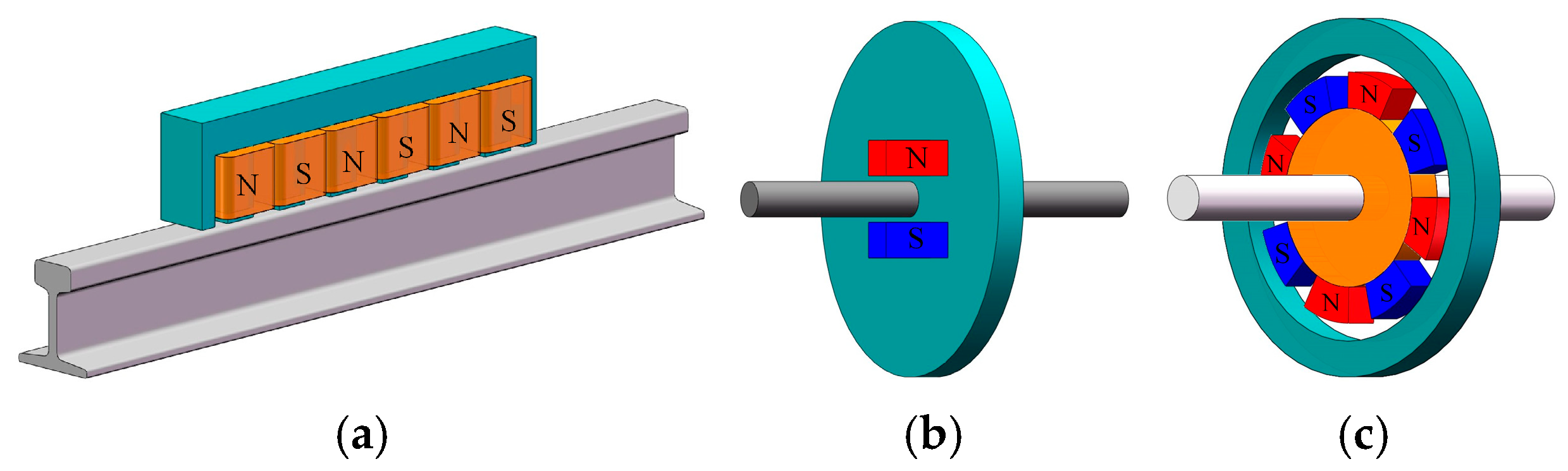
Based on the structural configuration, the ECB can be divided into two types: linear ECB and rotary ECB. Rotary types can be further divided into radial and axial types [7,8,9,10]. The linear ECB consists of the magnetic source mounted on the train bogie, with the rail serving as the secondary inductor. As the train travels, the relative motion between the magnetic source and the stationary rail induces eddy currents within the rail, which subsequently generate the required braking force. For the axial ECB, a metallic induction disk is mounted on the train axle as the secondary inductor, with the magnetic source positioned on one or both sides of the disk. As the train travels, the rotation of the axle drives the induction disk to move relative to the stationary magnetic sources. This interaction induces eddy currents within the disk, thereby generating the braking torque. For the radial ECB, the rotor core is fixed to the axle with the magnetic source mounted on its outer surface. The stator is secured to the bottom of the vehicle body via mechanical fixtures. As the axle rotates, the rotor core and the magnetic source rotate synchronously, creating relative motion against the stator. This process induces eddy currents within the inner surface of the stator, thereby generating the braking torque. These three structural configurations are shown in Figure 1.

Depending on the excitation method, the ECB can be divided into three types: electrical excitation, PM excitation, and hybrid excitation. The most commonly used electrical excitation ECB is DC excitation types. Traditional DC excitation ECBs convert all kinetic energy into heat within the secondary rail. This not only leads to excessive rail temperature rise, which may compromise track structural integrity at high speeds, but also requires a high-capacity DC power supply that adds significant weight to the vehicle [11,12]. PM excitation ECBs, while eliminating the need for an external excitation source, suffer from a lack of flux-adjusting capability. Furthermore, they face the risk of irreversible demagnetization under the extreme thermal conditions generated during continuous high-speed braking [6]. While hybrid excitation ECBs combine the advantages of both, they also increase the weight and complexity of the system [13,14,15].

Recent scholarly attention has shifted toward AC excitation ECBs [12,16,17,18]. While these systems offer the potential for partial energy recovery and reduced rail heating, they introduce a new challenge: the braking unit is inherently inductive, leading to a significantly low power factor. This results in an excessively large reactive power demand, forcing the onboard inverter to have a disproportionately high capacity, which increases cost and reduces system efficiency. Prior studies have largely failed to provide a coordinated solution that addresses both the thermal management of the rail and the optimization of the power supply hardware.

The purpose of this research is to develop and analyze a novel eddy current braking system (ECBS) with AC excitation and an auxiliary capacitor. By integrating excitation capacitors, this system aims to compensate for the reactive power demand in real-time, thereby significantly reducing the required inverter capacity. Simultaneously, the AC excitation facilitates the conversion of a portion of the train’s kinetic energy into storable electrical energy, providing a dual benefit of energy efficiency and thermal relief for the track.

To investigate the complex electromagnetic interactions within the proposed system, this study develops a rigorous 2D subdomain analytical framework that explicitly incorporates the longitudinal end effect. By solving the governing equations in each region and applying boundary conditions, the magnetic field distribution and air-gap flux linkages are accurately determined. Subsequently, an equivalent circuit model (ECM) is derived from the subdomain analytical results, where the impact of the longitudinal end effect is integrated into the secondary parameters. This ECM provides a computationally efficient tool to calculate the steady-state braking characteristics, power flow, and the impact of the auxiliary capacitor across a wide speed range. The proposed ECBS is primarily employed in high-speed trains as a critical braking method under high-speed or emergency conditions.

2. Analytical Method

2.1. Working Principle of ECBS

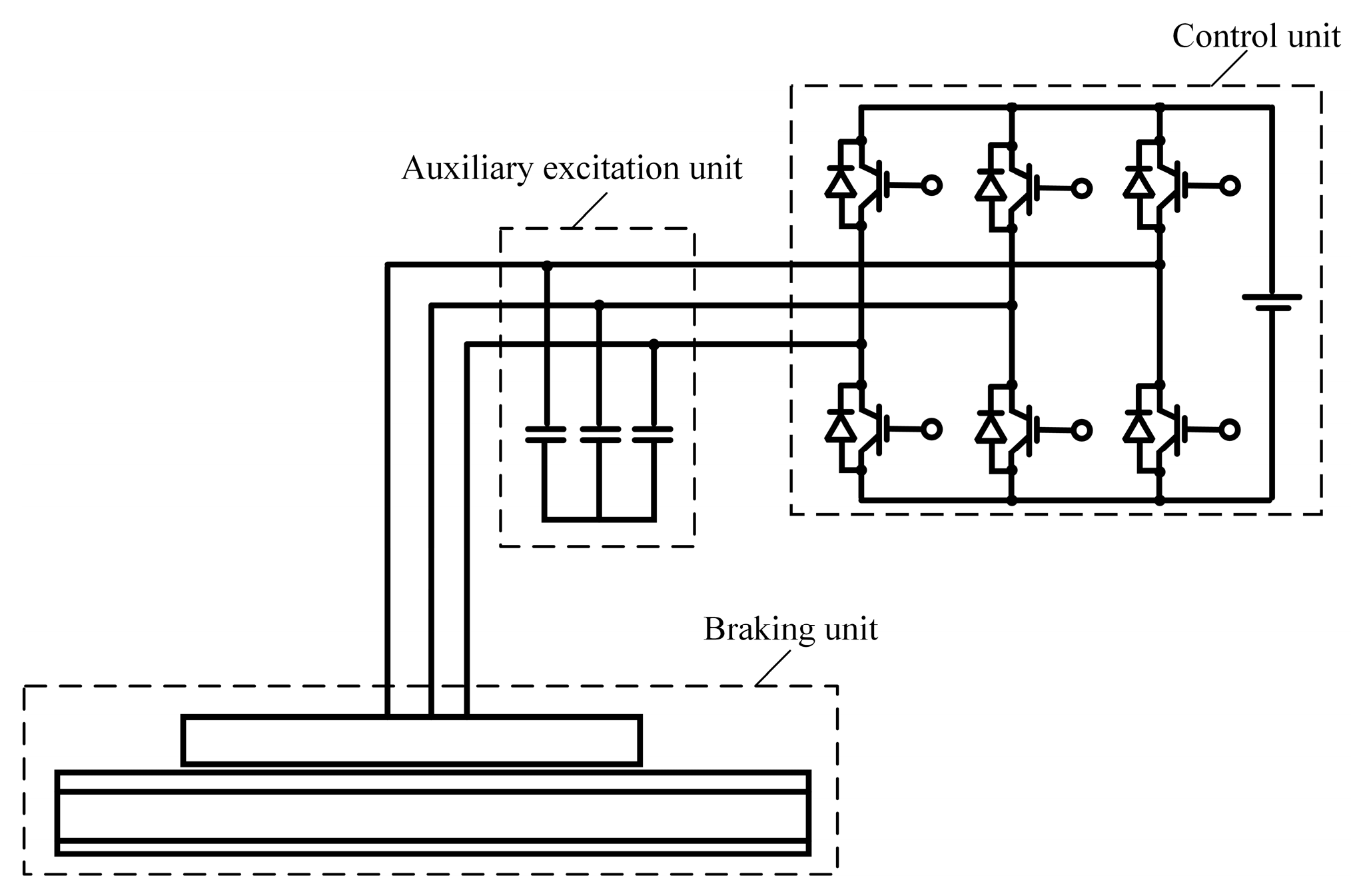
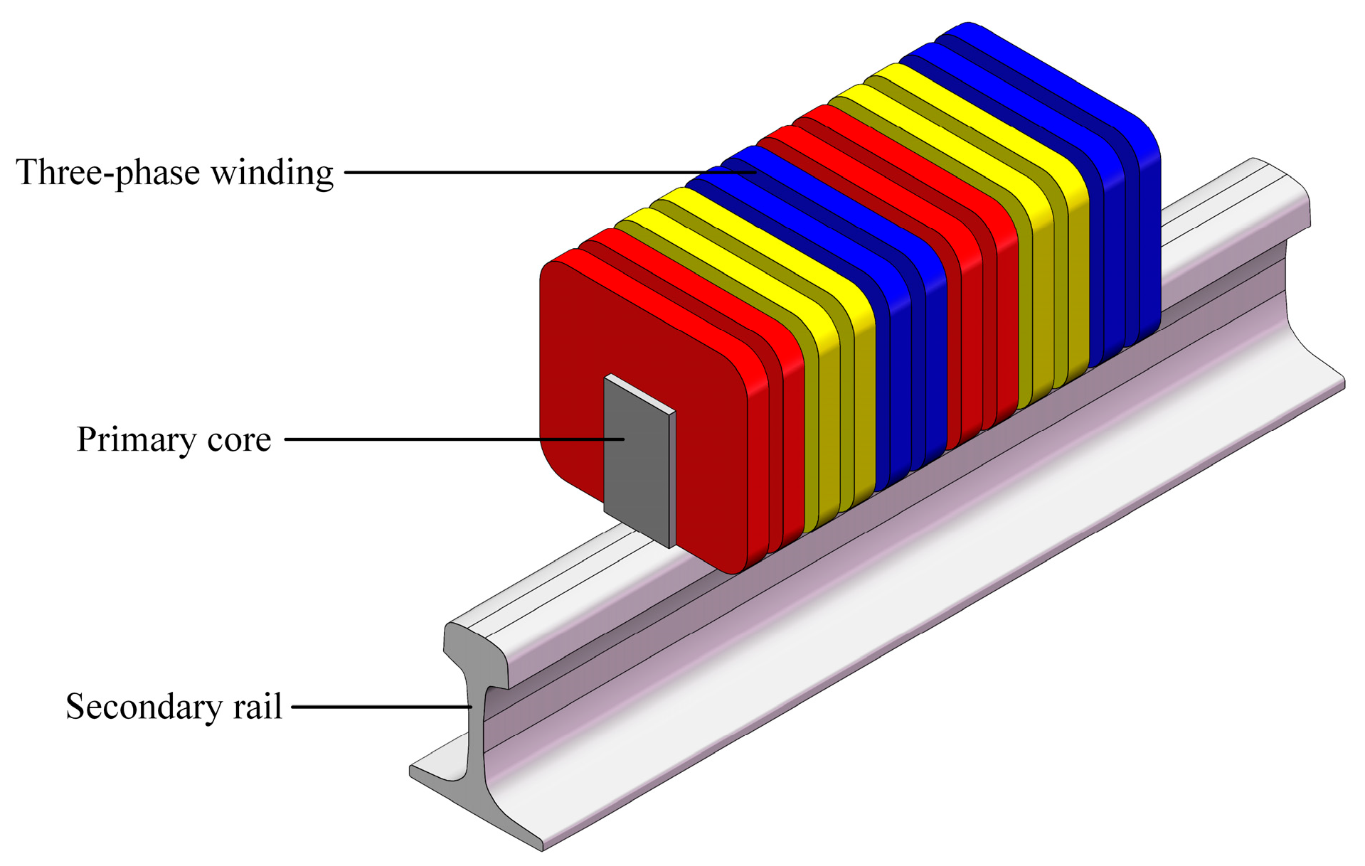
The ECBS with AC excitation and auxiliary capacitor proposed in this paper is shown in Figure 2, which includes three parts: control unit, braking unit and auxiliary excitation unit. The control unit includes a DC power supply and an excitation inverter. The braking unit consists of a primary mounted on the bogie and a rail secondary, which is essentially a three-phase linear induction motor with a toroidal winding structure. The auxiliary excitation unit includes a set of excitation capacitors. The structure of the braking unit is shown in Figure 3.

When the excitation current is applied to the primary winding of the braking unit, the traveling wave magnetic field is generated in the air gap between the primary and secondary. This traveling wave magnetic field links with the secondary rail, inducing the eddy current. The interaction between the eddy current and the traveling wave magnetic field generates the braking force opposite to the direction of train travel. This braking force acts on the primary of the braking unit, causing the train to decelerate. Simultaneously, the train’s kinetic energy is converted into the electrical energy output from the braking unit and the eddy current loss in the secondary rail. The output electrical energy can be consumed in the windings of the braking unit or stored in the onboard battery.

2.2. Subdomain Model

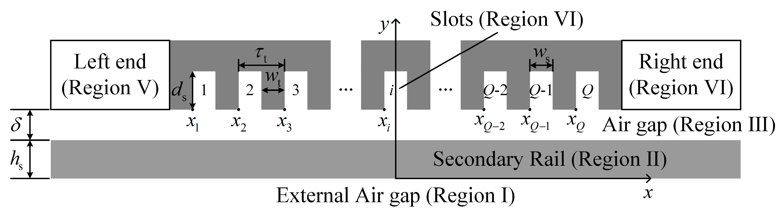
Figure 4 shows the proposed 2D subdomain model of the braking unit considering the longitudinal end effect, where Region I represents the external air gap, Region II the secondary rail, Region III the air gap, Region IV the slots, Region V the left end and Region VI the right end. The 2D analytical model is formulated with the following assumptions:

(1)

The transverse edge effect is neglected.

(2)

The permeability of the primary core is assumed to be infinite and the conductivity is assumed to be zero.

(3)

The permeability of the secondary rail is determined iteratively and the conductivity is assumed to be constant.

(4)

The vector magnetic potential and the current density have only z-direction components, while the magnetic flux density and the magnetic field strength have only x and y-direction components.

From the above assumptions, the magnetic vector potential in each region is given by

$${\nabla }^2{A}_z=0.$$

(1)

in Region I, Region III, Region V and Region VI,

$${\nabla }^2{A}_z=\mu \sigma \left[{\displaystyle \frac{\partial A_z}{\partial t}}+v{\displaystyle \frac{\partial A_z}{\partial x}}\right].$$

(2)

in Region II,

$${\nabla }^2{A}_z=-\mu J_{sz}.$$

(3)

in Region IV.

Herein, μ is the permeability of the secondary rail, σ is the conductivity of the secondary rail, v is the velocity of the secondary rail with respect to the primary, and J_sz is the current density in primary slots.

Region I: $x\in \left[-L,L\right]\wedge y\in \left[-\infty ,0\right]$ with ${\mu }_1={\mu }_0$.

The solution of governing Equation (1) is given by

$$A_z^{\mathrm{I}}\left(x,y\right)=A_0^{\mathrm{I}}y+B_0^{\mathrm{I}}+{\displaystyle \sum _{n=1}^{\infty }\left[\begin{array}{l}\left(A_n^{\mathrm{I}}{e}^{{\omega }_{n}y}+B_n^{\mathrm{I}}{e}^{-{\omega }_{n}y}\right)\cos {\omega }_n\left(x+L\right)\\ +\left(C_n^{\mathrm{I}}{e}^{{\omega }_{n}y}+D_n^{\mathrm{I}}{e}^{-{\omega }_{n}y}\right)\sin {\omega }_n\left(x+L\right)\end{array}\right]},$$

(4)

$${\omega }_n={\displaystyle \frac{n\mathrm{\pi }}{L}}.$$

(5)

where 2L is the length of the secondary rail, n is the spatial harmonic order, and $A_0^{\mathrm{I}}-D_n^{\mathrm{I}}$ are the complex integration constants in Region I.

Region II: $x\in \left[-L,L\right]\wedge y\in \left[0,h_{\mathrm{s}}\right]$ with ${\mu }_2={\mu }_0{\mu }_r$.

The solution of governing Equation (2) is given by

$$A_z^{\mathrm{II}}\left(x,y\right)=A_0^{\mathrm{II}}{e}^{r_{0}y}+B_0^{\mathrm{II}}{e}^{-r_{0}y}+{\displaystyle \sum _{n=1}^{\infty }\left[\begin{array}{l}\left(A_n^{\mathrm{II}}{e}^{r_{n}y}+B_n^{\mathrm{II}}{e}^{-r_{n}y}\right)\cos {\omega }_n\left(x+L\right)\\ +\left(C_n^{\mathrm{II}}{e}^{r_{n}y}+D_n^{\mathrm{II}}{e}^{-r_{n}y}\right)\sin {\omega }_n\left(x+L\right)\end{array}\right]},$$

(6)

$$r_n=\sqrt{{\omega }_n^2+\mathrm{j}\left({\omega }_{n}v-\omega \right){\mu }_0{\mu }_r\sigma }.$$

(7)

where h_s is the height of the secondary rail, ω is the primary angular frequency, μ_r is the relative permeability of the secondary rail, and $A_0^{\mathrm{II}}-D_n^{\mathrm{II}}$ are the complex integration constants in Region II.

Region III: $x\in \left[-L,L\right]\wedge y\in \left[h_{\mathrm{s}},h_{\mathrm{s}}+\delta \right]$ with ${\mu }_3={\mu }_0$.

The solution of governing Equation (1) is given by

$$A_z^{\mathrm{III}}\left(x,y\right)=A_0^{\mathrm{III}}y+B_0^{\mathrm{III}}+{\displaystyle \sum _{n=1}^{\infty }\left[\begin{array}{l}\left(A_n^{\mathrm{III}}{e}^{{\omega }_{n}y}+B_n^{\mathrm{III}}{e}^{-{\omega }_{n}y}\right)\cos {\omega }_n\left(x+L\right)\\ +\left(C_n^{\mathrm{III}}{e}^{{\omega }_{n}y}+D_n^{\mathrm{III}}{e}^{-{\omega }_{n}y}\right)\sin {\omega }_n\left(x+L\right)\end{array}\right]}.$$

(8)

where δ is the length of the air gap, $A_0^{\mathrm{III}}-D_n^{\mathrm{III}}$ are the complex integration constants in Region III.

Region IV: $x\in \left[x_i,x_i+w_{\mathrm{s}}\right]\wedge y\in \left[h_{\mathrm{s}}+\delta ,h_{\mathrm{s}}+\delta +d_{\mathrm{s}}\right]$ with ${\mu }_4={\mu }_0$.

The solution of governing Equation (3) is given by

$$A_z^{\mathrm{IV}\text{-}i}\left(x,y\right)=-{\displaystyle \frac{1}{2}}{\mu }_0{J}_z^{\mathrm{IV}\text{-}i}{y}^2+A_0^{\mathrm{IV}\text{-}i}y+B_0^{\mathrm{IV}\text{-}i}+{\displaystyle \sum _{m=1}^{\infty }\left[\left(A_m^{\mathrm{IV}\text{-}i}{e}^{{\omega }_{m}y}+B_m^{\mathrm{IV}\text{-}i}{e}^{-{\omega }_{m}y}\right)\cos {\omega }_m\left(x-x_i\right)\right]},$$

(9)

$${\omega }_m={\displaystyle \frac{m\mathrm{\pi }}{w_{\mathrm{s}}}},$$

(10)

$$x_i=-L+L_{\mathrm{end}}+{\displaystyle \frac{w_{\mathrm{t}}}{2}}+\left(i-1\right){\tau }_{\mathrm{t}},i=1-Q.$$

(11)

where $J_z^{\mathrm{IV}\text{-}i}$ is the current density of the i-th slot, τ_t is the tooth pitch, w_s is the width of slots, w_t is the width of teeth, d_s is the depth of slots, L_end is the length of the end region, m is the spatial harmonic order, and $A_0^{\mathrm{IV}\text{-}i}-B_m^{\mathrm{IV}\text{-}i}$ are the complex integration constants in Region IV.

Region V: $x\in \left[-L,-L+L_{end}\right]\wedge y\in \left[h_{\mathrm{s}}+\delta ,+\infty \right]$ with ${\mu }_5={\mu }_0$.

The solution of governing Equation (1) is given by

$$A_z^{\mathrm{V}}\left(x,y\right)=A_0^{\mathrm{V}}y+B_0^{\mathrm{V}}+{\displaystyle \sum }_{k=1}^{\infty }\left[\left(A_k^{\mathrm{V}}{e}^{{\omega }_{k}y}+B_k^{\mathrm{V}}{e}^{-{\omega }_{k}y}\right)\cos {\omega }_k\left(x+L\right)\right],$$

(12)

$${\omega }_k={\displaystyle \frac{k\mathrm{\pi }}{L_{\mathrm{end}}}}.$$

(13)

where k is the spatial harmonic order, and $A_0^{\mathrm{V}}-B_k^{\mathrm{V}}$ are the complex integration constants in Region V.

Region VI: $x\in \left[L-L_{end},L\right]\wedge y\in \left[h_{\mathrm{s}}+\delta ,+\infty \right]$ with ${\mu }_6={\mu }_0$.

The solution of governing Equation (1) is given by

$$A_z^{\mathrm{VI}}\left(x,y\right)=A_0^{\mathrm{VI}}y+B_0^{\mathrm{VI}}+{\displaystyle \sum }_{k=1}^{\infty }\left[\left(A_k^{\mathrm{VI}}{e}^{{\omega }_{k}y}+B_k^{\mathrm{VI}}{e}^{-{\omega }_{k}y}\right)\cos {\omega }_k\left(x-L+L_{\mathrm{end}}\right)\right].$$

(14)

where $A_0^{\mathrm{VI}}-B_k^{\mathrm{VI}}$ are the complex integration constants in Region VI.

Boundary conditions include two kinds: the vector magnetic potential and the tangential component of the magnetic field strength are continuous at the boundary. For ease of representation, we let $d_1=h_{\mathrm{s}}$, $d_2=h_{\mathrm{s}}+\delta$, $d_3=h_{\mathrm{s}}+\delta +d_{\mathrm{s}}$, $L_{\mathrm{c}}=L-L_{\mathrm{end}}$.

Boundary conditions are as follows:

• Boundary at $y=-\infty$:

  $$A_z^{\mathrm{I}}\left(x,-\infty \right)=0.$$

  (15)
• Boundary at $y=0$ between Region I and Region II

  $$A_z^{\mathrm{I}}\left(x,0\right)=A_z^{\mathrm{II}}\left(x,0\right).$$

  (16)

  $$H_x^{\mathrm{I}}\left(x,0\right)=H_x^{\mathrm{II}}\left(x,0\right).$$

  (17)
• Boundary at $y=d_1$ between Region II and Region III:

  $$A_z^{\mathrm{II}}\left(x,d_1\right)=A_z^{\mathrm{III}}\left(x,d_1\right).$$

  (18)

  $$H_x^{\mathrm{II}}\left(x,d_1\right)=H_x^{\mathrm{III}}\left(x,d_1\right).$$

  (19)
• Boundary at $y=d_2$ between Region III and Region IV, Region V, Region VI:

  $$\begin{array}{l}{A}_z^{\mathrm{IV}\text{-}i}\left(x,d_2\right)=A_z^{\mathrm{III}}\left(x,d_2\right),x_i<x<x_i+w_{\mathrm{s}},\\ A_z^{\mathrm{V}}\left(x,d_2\right)=A_z^{\mathrm{III}}\left(x,d_2\right),-L<x<-L_{\mathrm{c}},\\ A_z^{\mathrm{VI}}\left(x,d_2\right)=A_z^{\mathrm{III}}\left(x,d_2\right),L_{\mathrm{c}}<x<L.\end{array}$$

  (20)

  $$H_x^{\mathrm{III}}\left(x,d_2\right)=\left\{\begin{array}{l}{H}_x^{\mathrm{IV}\text{-}i}\left(x,d_2\right),x_i<x<x_i+w_{\mathrm{s}},\\ H_x^{\mathrm{V}}\left(x,d_2\right),-L<x<-L_{\mathrm{c}},\\ H_x^{\mathrm{VI}}\left(x,d_2\right),L_{\mathrm{c}}<x<L,\\ 0,\mathrm{elsewhere}.\end{array}\right.$$

  (21)
• Boundary at $y=d_3$ between Region IV and the primary yoke:

  $$H_x^{\mathrm{IV}\text{-}i}\left(x,d_3\right)=0,x_i<x<x_i+w_{\mathrm{s}}.$$

  (22)
• Boundary at $y=+\infty$:

  $$\begin{array}{l}{A}_z^{\mathrm{V}}(x,+\infty )=0,\\ A_z^{\mathrm{VI}}(x,+\infty )=0.\end{array}$$

  (23)

To account for the magnetic saturation of the secondary rail, the permeability is treated as a variable linked to the local field intensity. Specifically, an iterative procedure is employed: an initial permeability is first assigned to solve the subdomain equations, from which the magnetic flux density B in the rail is obtained. This B value is then used to look up the corresponding permeability on the B-H curve for the subsequent iteration. This recursive update continues until the discrepancy between the assumed and calculated permeability is minimized, ensuring that the nonlinear material properties are accurately reflected in the final field solution.

When the braking unit is fed by three-phase sinusoidal current, the current density in the i-th slot is defined as follows:

$$J_z^{\mathrm{IV}\text{-}i}={\displaystyle \frac{N_{\mathrm{c}}}{S_{\mathrm{slot}}}}{M}^T\cdot \sqrt{2}{I}_{\mathrm{rms}}\cdot {\left[\begin{array}{ccc}1& e^{-\mathrm{j}{\displaystyle \frac{2\mathrm{\pi }}{3}}}& e^{\mathrm{j}{\displaystyle \frac{2\mathrm{\pi }}{3}}}\end{array}\right]}^T.$$

(24)

where N_c is the number of conductors in the slot, S_slot is the area of the slot, M is the matrix connection between the phase current and primary slots, I_rms is the effective value of the phase current.

The connection matrix of one pole is expressed as follows:

$$M=\left[\begin{array}{cccccc}1& 1& 0& 0& 0& 0\\ 0& 0& -1& -1& 0& 0\\ 0& 0& 0& 0& 1& 1\end{array}\right].$$

(25)

Based on the governing equation of each region (4), (6), (8), (9), (12), (14) and boundary conditions (15)–(23), all the integration constants can be obtained. Detailed solution steps are shown in the Appendix A. Therefore, the magnetic flux density in the air gap can be given by

$$B_x^{\mathrm{III}}\left(x,y\right)={\displaystyle \frac{\partial A_z^{\mathrm{III}}\left(x,y\right)}{\partial y}}=A_0^{\mathrm{III}}+{\displaystyle \sum _{n=1}^{\infty }{\omega }_n\left[\begin{array}{l}\left(A_n^{\mathrm{III}}{e}^{{\omega }_{n}y}-B_n^{\mathrm{III}}{e}^{-{\omega }_{n}y}\right)\cos {\omega }_n\left(x+L\right)\\ +\left(C_n^{\mathrm{III}}{e}^{{\omega }_{n}y}-D_n^{\mathrm{III}}{e}^{-{\omega }_{n}y}\right)\sin {\omega }_n\left(x+L\right)\end{array}\right]}.$$

(26)

$$B_y^{\mathrm{III}}\left(x,y\right)=-{\displaystyle \frac{\partial A_z^{\mathrm{III}}\left(x,y\right)}{\partial x}}={\displaystyle \sum _{n=1}^{\infty }{\omega }_n\left[\begin{array}{l}\left(A_n^{\mathrm{III}}{e}^{{\omega }_{n}y}+B_n^{\mathrm{III}}{e}^{-{\omega }_{n}y}\right)\sin {\omega }_n\left(x+L\right)\\ -\left(C_n^{\mathrm{III}}{e}^{{\omega }_{n}y}+D_n^{\mathrm{III}}{e}^{-{\omega }_{n}y}\right)\cos {\omega }_n\left(x+L\right)\end{array}\right]}.$$

(27)

According to the Maxwell stress equation, the braking force and the normal force can be obtained:

$$F_x={\displaystyle \frac{W_c}{2{\mu }_0}}{\displaystyle {\int }_{-L}^L\mathrm{Re}\left(B_x^{\mathrm{III}}\left(x,0\right)B_y^{\mathrm{III}}-\left(x,0\right)\right)}\mathrm{d}x.$$

(28)

$$F_y={\displaystyle \frac{W_c}{4{\mu }_0}}{\displaystyle {\int }_{-L}^L\left({\left|B_x^{\mathrm{III}}\left(x,0\right)\right|}^2-{\left|B_y^{\mathrm{III}}\left(x,0\right)\right|}^2\right)}\mathrm{d}x.$$

(29)

where W_c is the width of the primary core.

2.3. Equivalent Circuit

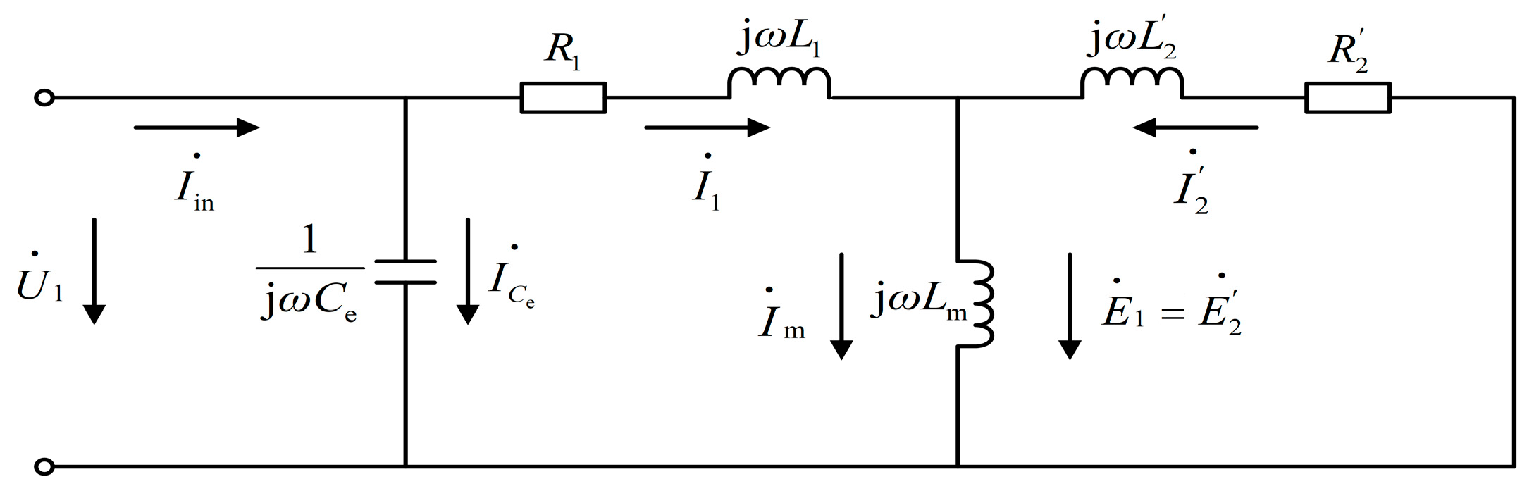
Unlike the equivalent circuit of a traditional induction motor, the equivalent circuit of the ECBS proposed in this paper takes into account the longitudinal end effect, as shown in Figure 5. R₁ is the primary resistance, L₁ is the primary leakage inductance, L_m is the magnetizing inductance, R₂′ is the secondary resistance referred to the primary, L₂′ is the secondary leakage inductance referred to the primary, and C_e is the excitation capacitance. R₁ can be determined by a classical analytical formula. In a 2D analytical model, L₁ only considers the slot leakage inductance and can be obtained by slot leakage permeance. C_e is determined according to the design specifications. The remaining parameters can be obtained from the subdomain model results as follows.

According to the Stokes theorem, the complex flux linkage in the i-th slot can be given by

$${\psi }^{\mathrm{IV}\text{-}i}={\displaystyle \frac{N_{\mathrm{c}}{W}_{\mathrm{c}}}{S_{\mathrm{slot}}}}{\displaystyle \underset{x_i}{\overset{x_i+w_{\mathrm{s}}}{\int }}{\displaystyle \underset{d_2}{\overset{d_3}{\int }}{A}_z^{\mathrm{IV}\text{-}i}\left(x,y\right)}}\mathrm{d}y\mathrm{d}x.$$

(30)

The complex flux linkage of each phase can be obtained

$${\left[\begin{array}{ccc}{\psi }_A& {\psi }_B& {\psi }_C\end{array}\right]}^T=M\cdot {\left[\begin{array}{ccccc}{\psi }^{\mathrm{IV}\text{-}1}& {\psi }^{\mathrm{IV}\text{-}2}& \dots & {\psi }^{\mathrm{IV}\text{-}\left(Q-1\right)}& {\psi }^{\mathrm{IV}\text{-}Q}\end{array}\right]}^T.$$

(31)

When the braking unit is in no-load condition, the secondary branch is open-circuited. The complex phase flux linkage satisfies the following relationship

$$\mathrm{j}\omega {\psi }_1=-E_1+\mathrm{j}\omega L_1{I}_1.$$

(32)

$$E_1=-\mathrm{j}\omega L_{\mathrm{m}}{I}_1.$$

(33)

Rearranging (32) and (33) yields

$$L_{\mathrm{m}}={\displaystyle \frac{{\psi }_1}{I_1}}-L_1.$$

(34)

Since the three-phase flux linkages are asymmetrical, the positive-sequence component is adopted here

$${\psi }_1={\displaystyle \frac{1}{3}}\left({\psi }_A+a{\psi }_B+a^2{\psi }_C\right).$$

(35)

where $a=e^{\mathrm{j}{\displaystyle \frac{2\mathrm{\pi }}{3}}}$, $a^2=e^{-\mathrm{j}{\displaystyle \frac{2\mathrm{\pi }}{3}}}$.

As shown in Figure 4, when the braking unit is in a load condition, the circuit equations are given as follows, in addition to (32):

$$U_1=-E_1+\left(R_1+\mathrm{j}\omega L_1\right)I_1.$$

(36)

$$E_1=E_2^{\prime }=-\mathrm{j}\omega L_{\mathrm{m}}{I}_{\mathrm{m}}.$$

(37)

$$E_2^{\prime }=I_2^{\prime }\left(R_2^{\prime }+\mathrm{j}\omega L_2^{\prime }\right).$$

(38)

$$I_1+I_2^{\prime }=I_{\mathrm{m}}$$

(39)

Thus, by substituting the positive-sequence flux linkages under different operating conditions into the aforementioned equations, the secondary parameters can be obtained.

3. Results

The obtained equivalent circuit parameters can be utilized to calculate the braking characteristics of the ECBS. As long as these three parameters (f, v, I₁) are known, the braking characteristics are uniquely determined. The dimensional parameters of the braking unit are shown in

Table 1. Dimensional Parameters.

Quantity	Symbol	Value
Number of slots	Q	36
Tooth pitch	τt	32 mm
Slot width	ws	16 mm
Tooth width	wt	16 mm
Slot depth	ds	55 mm
Yoke height	hy	55 mm
Width of primary core	Wc	70 mm
Length of air gap	Δ	6.5 mm
Height of secondary rail	hs	35 mm

.

3.1. Under Inverter-Only Supply Conditions

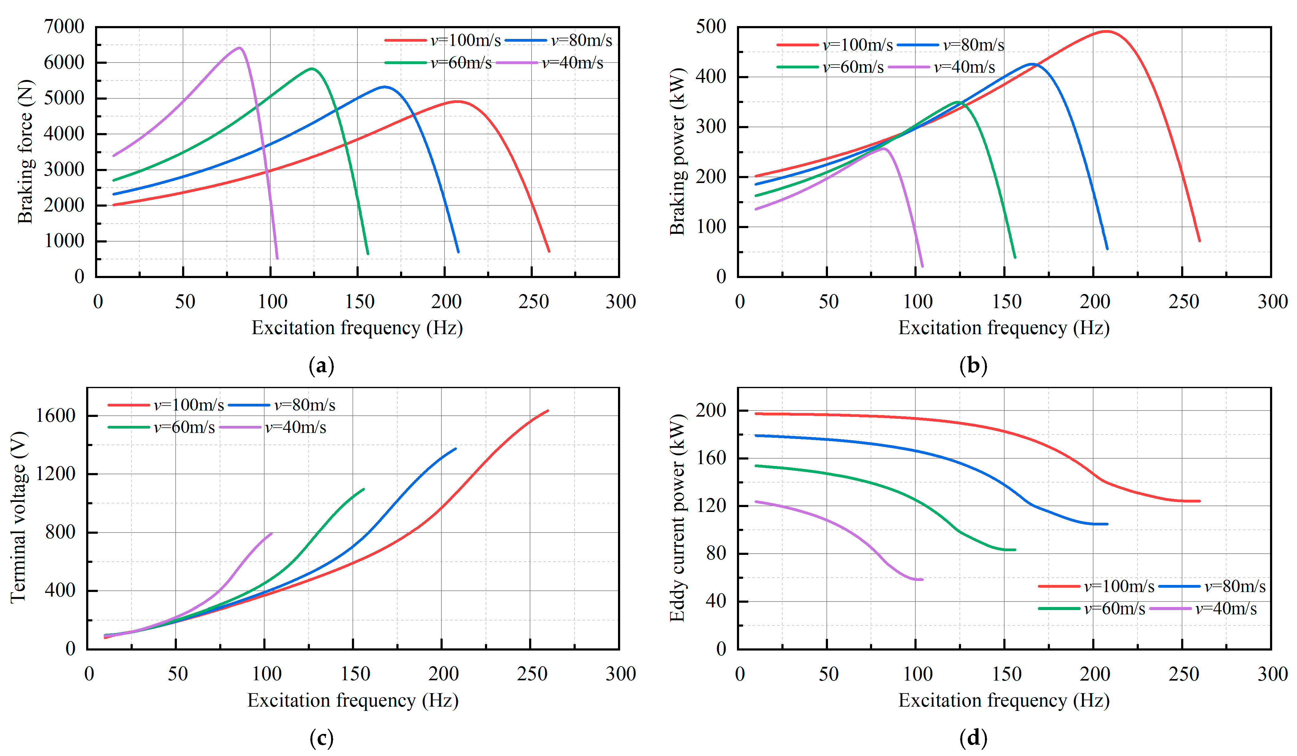
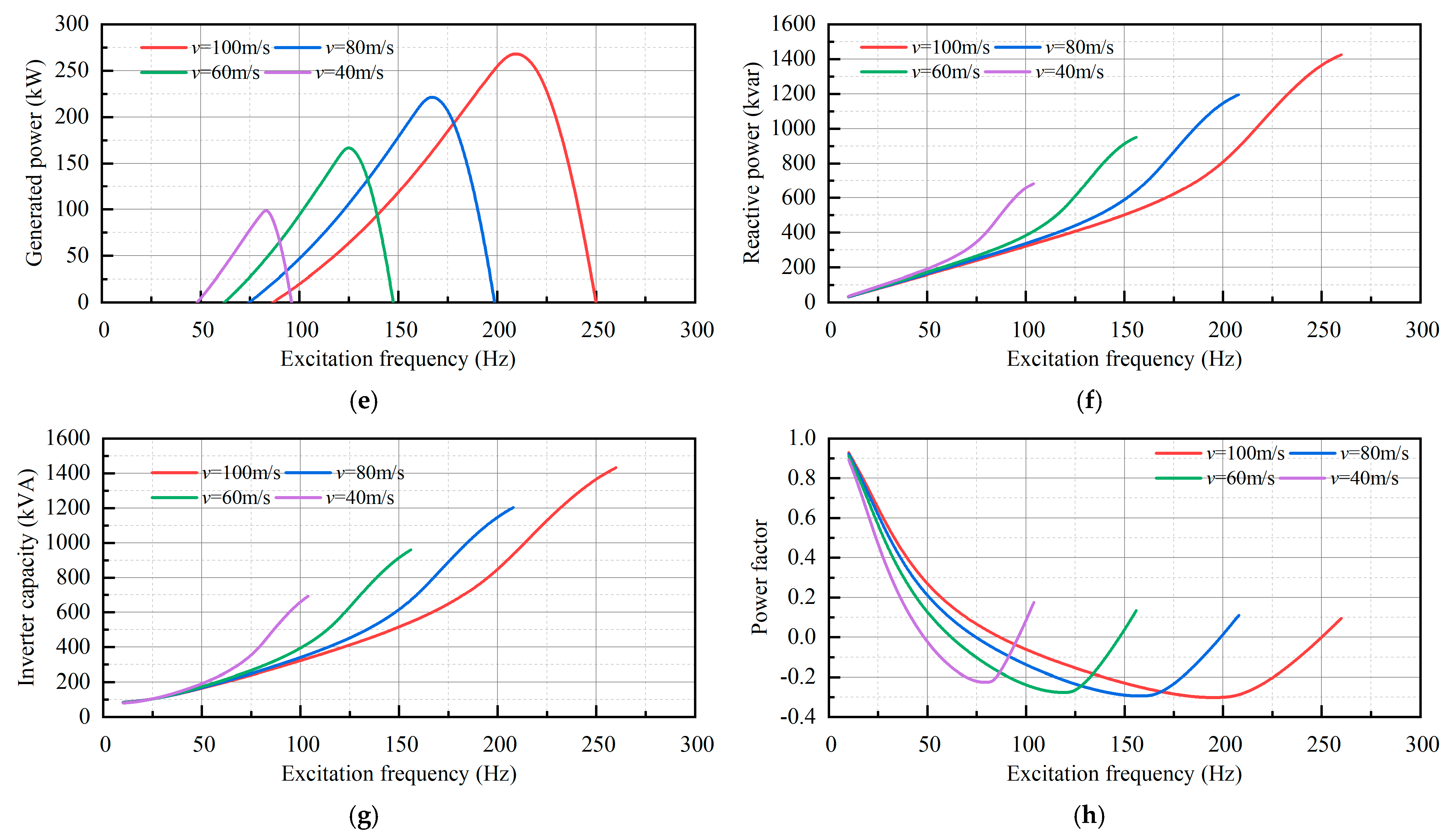
Figure 6 shows the braking characteristics under inverter-only supply conditions. The phase current is fixed at I_{1_rms} = 291.6 A. The braking force first increases and then decreases with the increment of the excitation frequency, and decays to zero when the synchronous speed corresponding to the excitation frequency approaches the actual operating speed. In addition, as the operating speed decreases, the peak braking force increases. The braking power exhibits a similar trend to that of the braking force. However, as the operating speed decreases, the peak braking power diminishes. The terminal voltage increases continuously with the excitation frequency. However, at a fixed excitation frequency, a lower operating speed results in a higher terminal voltage. The eddy current power decreases with the increase of excitation frequency, and also diminishes as the operating speed drops. The generated power is positive only within a certain range of excitation frequencies and exhibits a trend of first increasing and then decreasing as the frequency rises. Moreover, the peak generated power diminishes as the operating speed decreases. The inverter output reactive power and the inverter capacity exhibit the same variation trend, both increasing with the increment of excitation frequency. The power factor is negative within a specific range of excitation frequencies, which corresponds to the interval where the generated power is positive.

3.2. Under Capacitor-Assisted Excitation Conditions

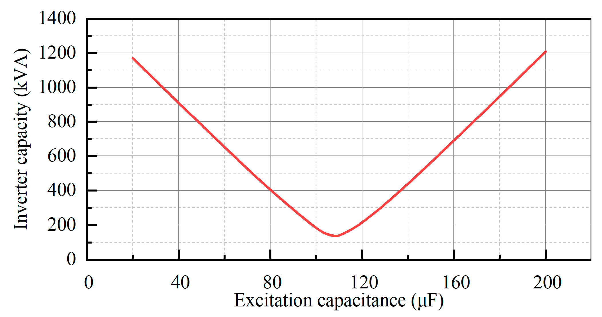
As shown in Figure 6f,g, both the reactive power supplied by the inverter and the inverter capacity increase with the increment of operating speed and excitation frequency. Therefore, we fix the operating condition at v = 100 m/s, f = 260 Hz, and I_{1_rms} = 291.6 A. Figure 7 illustrates the curves of inverter capacity versus excitation capacitance under this operating condition. It can be seen that, when the capacitance is close to 108 μF, the inverter capacity reaches its minimum, which is approximately 137 kVA. Compared with the inverter-only supply condition, the inverter capacity is reduced by 90%.

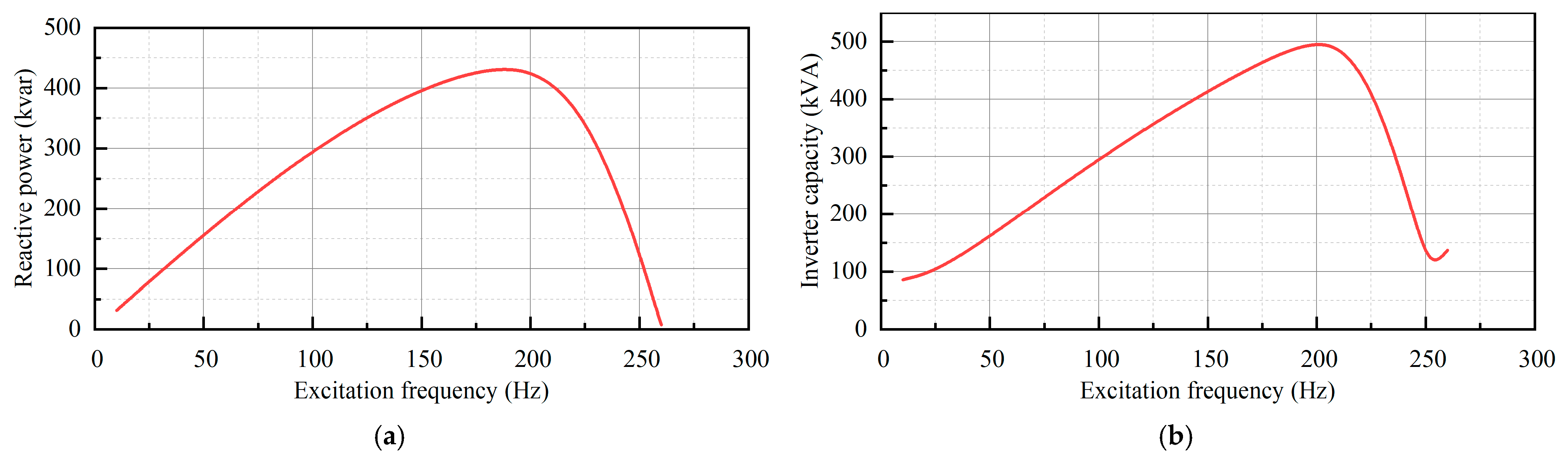
Figure 8 illustrates the curves of the inverter output reactive power and the inverter capacity versus excitation frequency when C_e = 108 μF, v = 100 m/s, and I_{1_rms} = 291.6 A. It can be seen that the reactive power supplied by the inverter first increases and then decreases with the excitation frequency. However, it remains significantly lower than that provided in the inverter-only case. The inflection point occurs because although the reactive power supplied by the excitation capacitor increases with the excitation frequency, it cannot fully satisfy the reactive power demand of the braking unit. Consequently, before the inflection point, the reactive power supplied by the inverter increases. As the excitation frequency continues to rise, the reactive power supplied by the capacitor keeps increasing at a rate that exceeds the demand of the braking unit. Therefore, the reactive power output from the inverter begins to decrease. The inward inflection on the right side in Figure 8b is caused by the increase in active power supplied by the inverter as the synchronous speed approaches the actual operating speed.

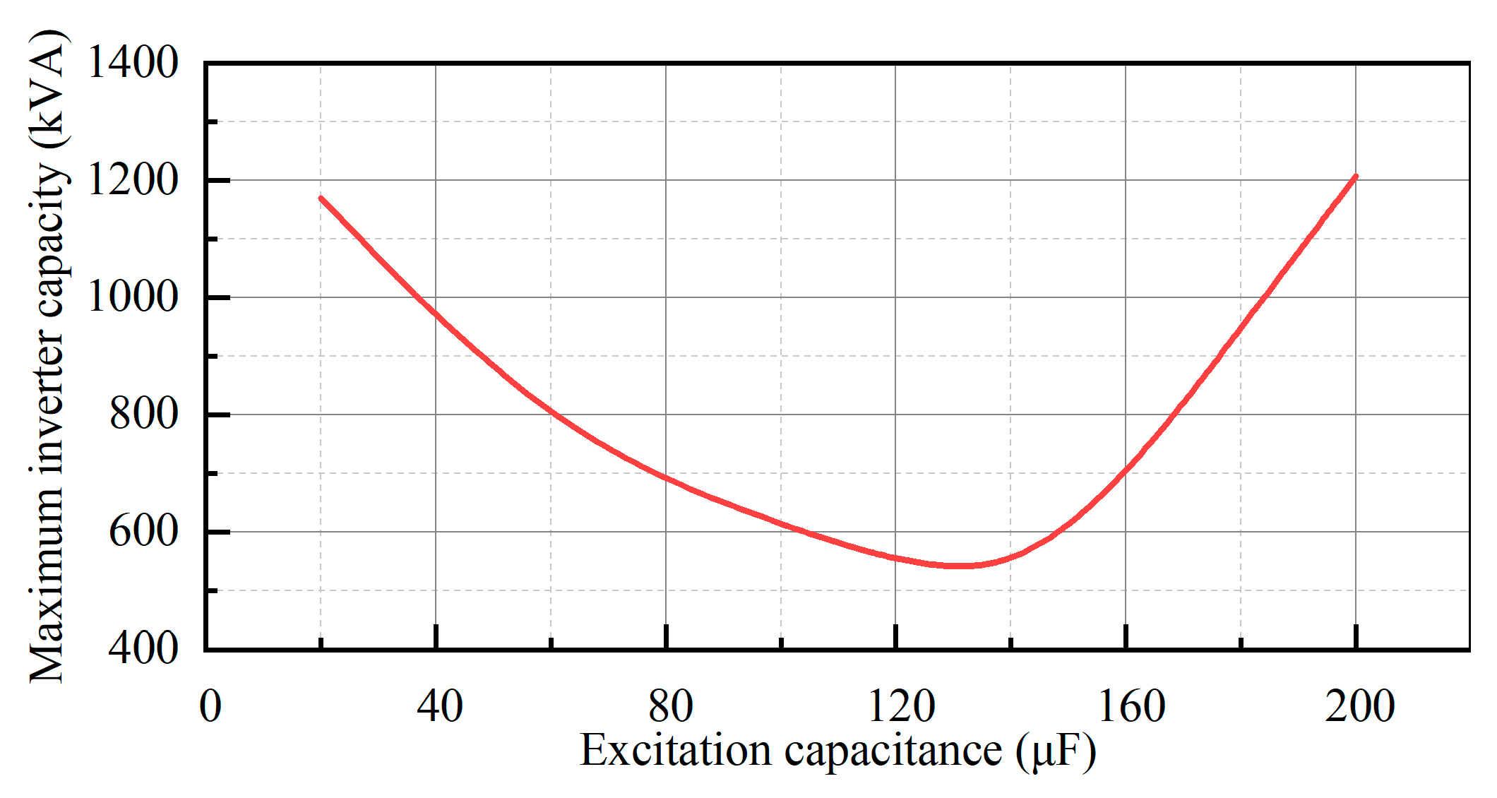
Considering that the inverter capacity exhibits two inflection points when the excitation capacitance is fixed, the maximum values of the inverter capacity across the entire speed range and the full excitation frequency spectrum were extracted for different capacitance values. As shown in Figure 9, the optimal capacitance value is defined as the one that minimizes the maximum inverter capacity. The optimal capacitance value is about 134 μF.

3.3. FEM Validation and Results

A 2D finite element model (FEM) is established to verify the accuracy of the proposed ECM. The 2D FEM is shown in Figure 10. The FEM simulation is performed using JMAG Designer version 24.0.

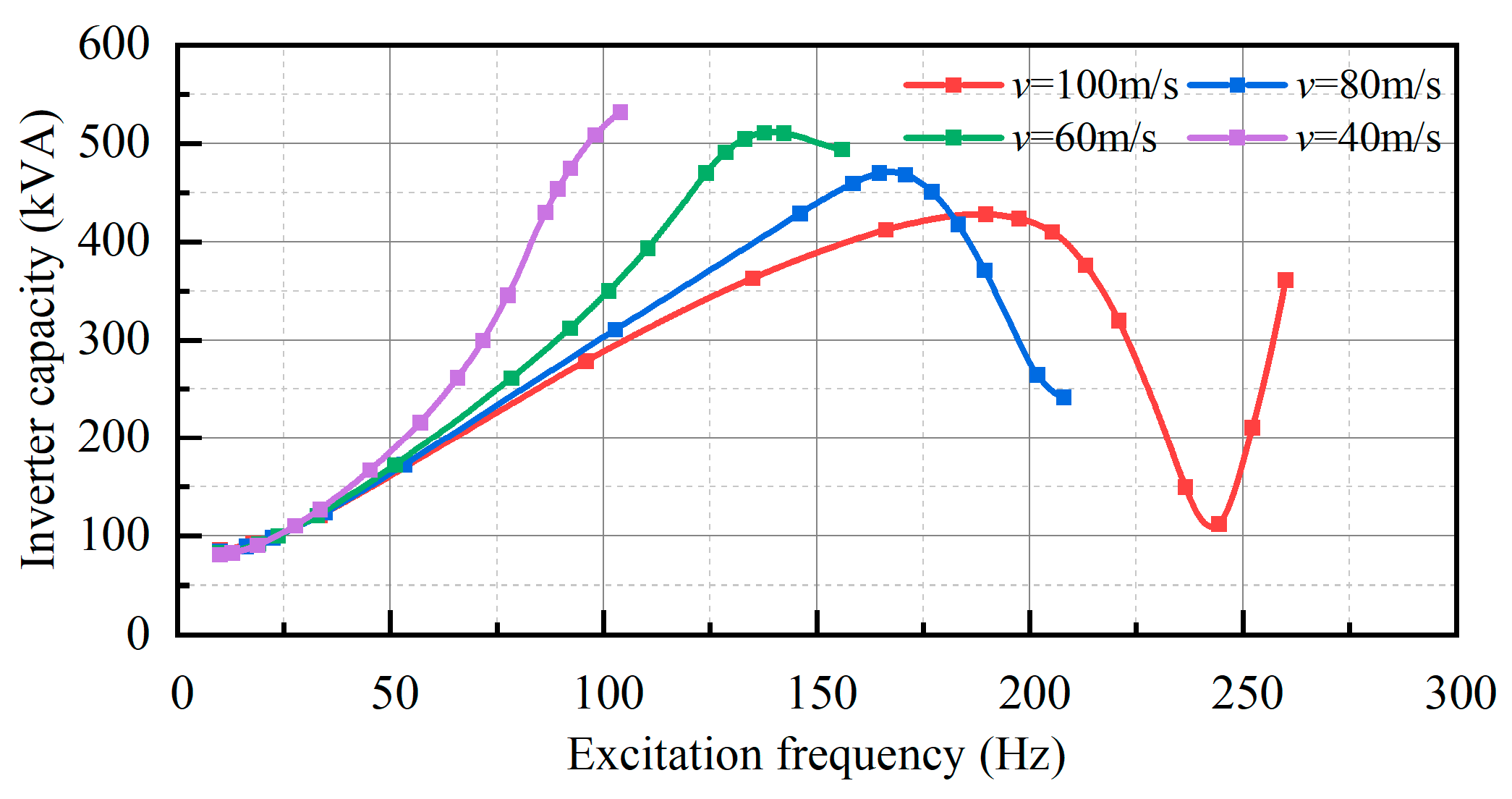
Figure 11 illustrates the curve of the inverter capacity versus excitation frequency when C_e = 134 μF and I_{1_rms} = 291.6 A. As can be seen, with a capacitance of 134 μF, the FEM results indicate that the required inverter capacity reaches its maximum at v = 40 m/s when the slip is close to zero. This peak value is approximately 535 kVA, which is in close agreement with the inverter capacity corresponding to the optimal capacitance in Figure 9. This validates the accuracy of the proposed ECM.

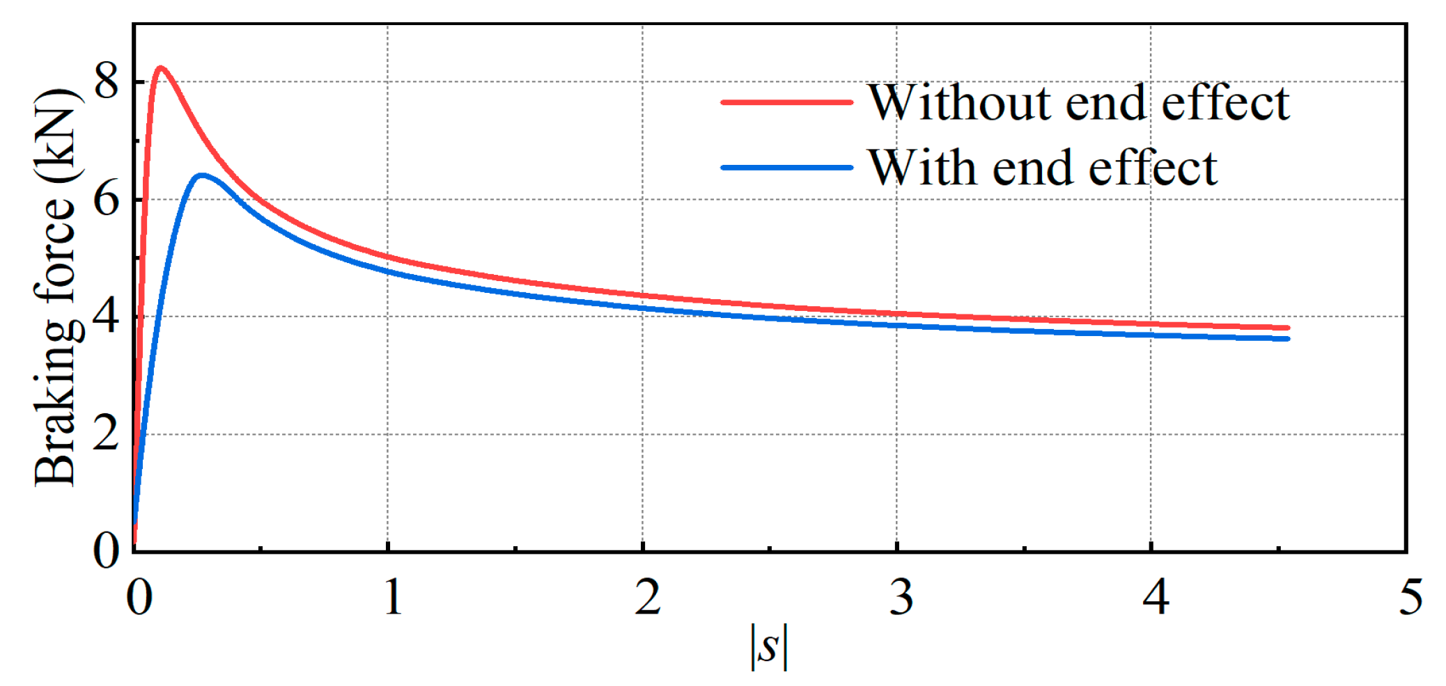
Figure 12 shows the braking force calculated by ECM which accounts for the longitudinal end effect and FEM with translation periodic boundary which neglects the longitudinal end effect. It can be seen that the proposed ECM fully incorporates the influence of the longitudinal end effect, which significantly reduces the braking force in the low-slip region.

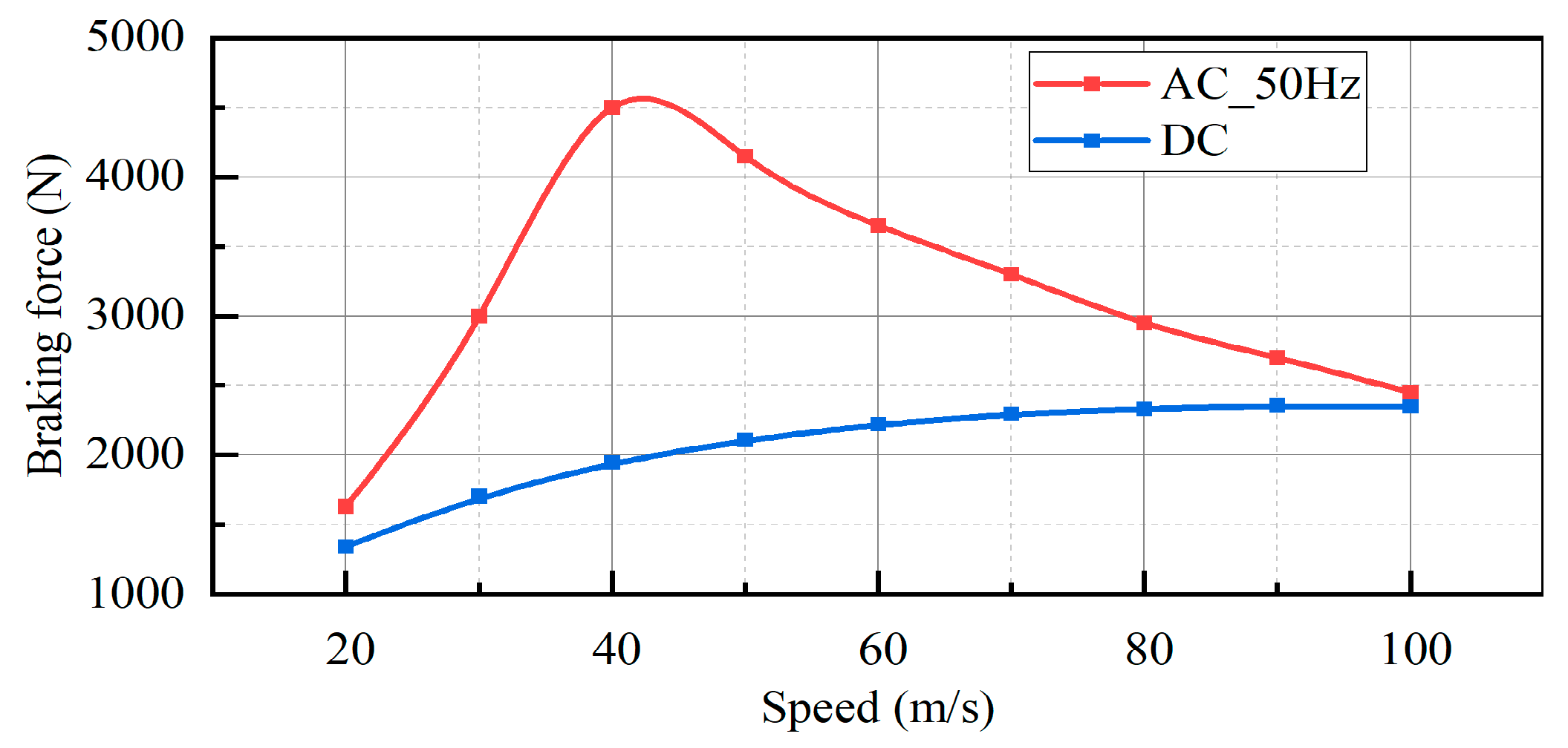
In addition, the braking characteristics of DC excitation and AC excitation were compared. The geometric structure of the braking unit remains unchanged, with only the AC excitation being replaced by DC excitation while maintaining a constant current density. Figure 13 compares the braking force curves between DC excitation and AC excitation. It is evident that the braking force under AC excitation is significantly higher than that under DC excitation.

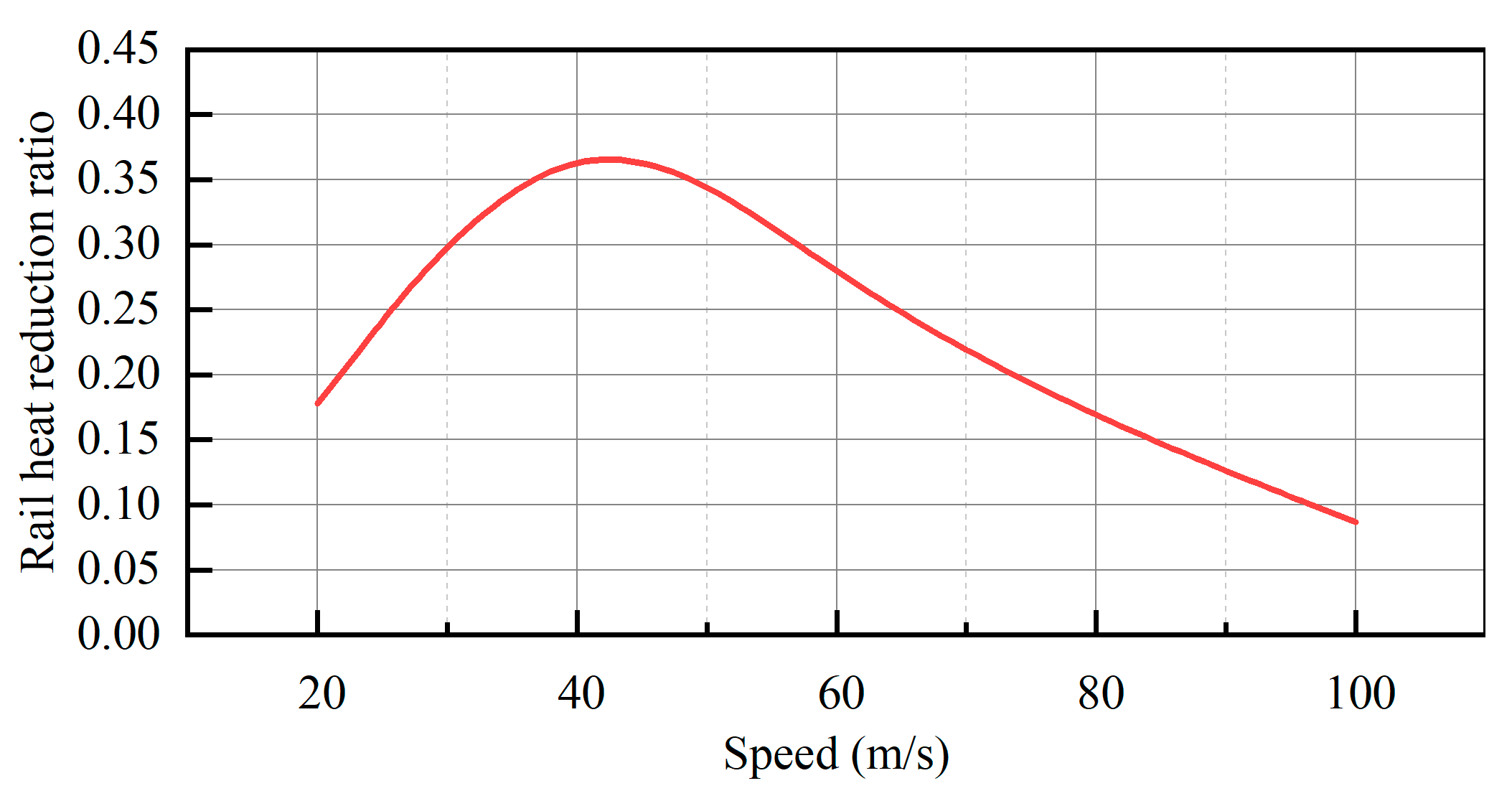
We define the rail heat reduction ratio as the proportion of kinetic energy converted into feedback electrical energy rather than being dissipated as heat in the secondary rail. Figure 14 illustrates the curve of the rail heat reduction ratio when f = 50 Hz and I_{1_rms} = 291.6 A. As illustrated in the figure, AC excitation can feed a portion of the kinetic energy back to the primary side, with a maximum conversion efficiency of 36%. In contrast, DC excitation converts the entire kinetic energy into thermal energy within the rail, resulting in a rail heat reduction ratio of zero, which significantly increases the rail temperature rise.

4. Discussion

The results confirm that the proposed ECBS with AC excitation and auxiliary capacitor significantly optimizes the braking performance. Compared to conventional ECBs with DC excitation, this system enables energy recovery and reduces rail thermal stress. Most notably, the 90% reduction in inverter capacity achieved by the 108 μF capacitor provides a feasible path for high-power braking in space-constrained locomotives.

This system is ideally suited for high-speed railway (up to 100 m/s). In practice, the recovered electrical energy can power auxiliary loads, improving the overall efficiency of the train. While adding capacitors introduces incremental hardware, the drastic downsizing of the power inverter leads to a more cost-effective and lighter braking suite.

4.1. Engineering Limitations and Operational Challenges

Despite its advantages, the practical implementation of the proposed ECBS faces several engineering challenges:

(1)

Parameter Sensitivity: The LC resonance is sensitive to variations in the air-gap length or temperature-induced changes in rail conductivity. Such deviations may shift the optimal operating point and reduce compensation efficiency.

(2)

Transient Overvoltage Risks: During sudden changes in operating modes or frequency switching, the interaction between the inductive braking unit and capacitors may trigger short-term overvoltages, requiring robust insulation coordination.

(3)

System Complexity: Compared to DC systems, the AC-excited configuration requires more sophisticated control algorithms to synchronize the excitation frequency with the train speed to maintain peak braking force.

4.2. Future Work

To further enhance the reliability of braking systems for diverse electric locomotives, future research will be strategically directed toward three key areas: first, the development of robust transient protection schemes, specifically focusing on surge suppression and insulation coordination to safeguard capacitor-assisted circuits against operational switching transients; second, the implementation of adaptive control algorithms featuring real-time resonance tracking to maintain a high power factor and compensation efficiency despite environmental fluctuations or parameter drifts; and finally, the integration with hybrid braking systems, where coordinated control strategies will be established between the AC-ECBS, conventional friction brakes, and regenerative systems to ensure fail-safe operation and stable deceleration across all speed ranges and operating modes.

5. Conclusions

In this paper, a novel eddy current braking system (ECBS) with AC excitation and auxiliary capacitor is proposed and analyzed, providing a high-performance solution for non-contact deceleration in high-speed rail applications (up to 100 m/s). Based on the 2D subdomain analytical model that explicitly accounts for the longitudinal end effect and the derived equivalent circuit, the results confirm that the proposed system significantly optimizes both hardware requirements and thermal management. Most notably, the implementation of an auxiliary capacitor significantly optimizes the hardware requirement. At the specific operating condition of v = 100 m/s and f = 260 Hz, an optimal capacitance of 108 μF reduces the required inverter capacity by 90% (from 1422 kVA to 137 kVA). However, considering the entire speed range and excitation frequency spectrum, a global optimal capacitance of 134 μF is determined to minimize the maximum required inverter capacity, ensuring system stability and efficiency across all operating modes. Furthermore, the AC configuration achieves a peak braking force of 6400 N with a maximum energy recovery efficiency of 36%, effectively mitigating rail thermal stress. The high degree of consistency between the analytical equivalent circuit and the FEM verification conducted in JMAG Designer version 24.0 ensures that this modeling framework provides a reliable and computationally efficient tool for the preliminary electromagnetic design of next-generation, energy-efficient braking systems.

References

1. Gulec, M.; Aydin, M.; Sergeant, P. Eddy Current Brakes: A Review on Working Principles and Technology Evolution. In Proceedings of the 2022 International Conference on Electrical Machines (ICEM), Valencia, Spain, 5–8 September 2022; pp. 441–447. [Google Scholar] [CrossRef]
2. Choi, G.; Jang, G.-H. A Hybrid Brake System for E-Scooters: Design, Optimization, and Performance-Validation Study of Axial Flux Eddy-Current Brake with Halbach Array. IEEE Access 2026, 14, 16233–16244. [Google Scholar] [CrossRef]
3. Li, X.; Zhai, X.; Yang, F.; Chen, L. A Model Prediction Method for the Electromagnetic Force of an Axial Flux Eddy Current Brake Based on the ISSA Algorithm. IEEE Trans. Magn. 2025, 61, 8001314. [Google Scholar] [CrossRef]
4. Kundu, J.; Kumar, P.; Srivastava, R.K. Design, Control and Real-Time Simulation of an Eddy Current Brake for High Speed Rotating Machines. In Proceedings of the 2025 IEEE Industry Applications Society Annual Meeting (IAS), Taipei, Taiwan, 15–20 June 2025; pp. 1–5. [Google Scholar] [CrossRef]
5. Sano, S.; Arita, H.; Kosaka, T. Estimation of Eddy Current Load Device Torque Applied to High-Speed Motors Using Magnetic Field-Thermal Coupled Analysis. In Proceedings of the 2025 28th International Conference on Electrical Machines and Systems (ICEMS), Busan, Republic of Korea, 16–19 November 2025; pp. 1213–1218. [Google Scholar] [CrossRef]
6. Kou, B.; Zhang, H.; Yin, X.; Zhou, Y.; Li, C. Research on Long Stroke Moving Secondary Permanent Magnet Linear Eddy Current Brake. Trans. Electr. Mach. Syst. 2019, 3, 19–29. [Google Scholar] [CrossRef]
7. Canova, A.; Vusini, B. Analytical Modeling of Rotating Eddy-Current Couplers. IEEE Trans. Magn. 2005, 41, 24–35. [Google Scholar] [CrossRef]
8. Ye, L.; Li, D.; Ma, Y.; Jiao, B. Design and Performance of a Water-Cooled Permanent Magnet Retarder for Heavy Vehicles. IEEE Trans. Energy Convers. 2011, 26, 953–958. [Google Scholar] [CrossRef]
9. Guo, W.; Li, X.; Gao, Z. Study on Thermal Decay of Braking Torque Novel Fully Water-Cooled Eddy Current Brakes under Extreme Conditions. IEEE Trans. Transp. Electrif. 2025, 12, 2704–2715. [Google Scholar] [CrossRef]
10. Hassanpour, H.; Ebrahimi-Nejad, S.; Mollajafari, M. Parametric Study of Permanent Magnet Eddy Current Brake Considering Demagnetization, Temperature, Edge, and Skin Effects: Numerical and Experimental Investigation. Appl. Eng. Sci. 2025, 22, 100235. [Google Scholar] [CrossRef]
11. Wang, J.; Fang, X.; Cui, C.; Yang, Z.; Lin, F.; Zhu, N.; Sun, H. Nonlinear Analytical Modeling of Normal Force in Eddy Current Braking for Maglev Trains. IEEJ J. IA 2025, 14, 659–669. [Google Scholar] [CrossRef]
12. Li, J.; Li, Y.; Xu, J.; Luo, J.; Xu, S.; Li, Y.; Zeng, M.; Yu, H.; Cui, L.; Song, X.; et al. Calculation and Characterization of Braking Performance for Rail Eddy Current Brake with AC Excited Ring-Winding Armature. IEEE Trans. Ind. Appl. 2023, 59, 1614–1625. [Google Scholar] [CrossRef]
13. Cui, C.; Fang, X.; Wang, J.; Li, Y.; Yang, Z.; Lin, F. A Linear Eddy Current Braking System with Normal Force Suppression Function for Electrodynamic Suspension Train. IEEE Trans. Magn. 2025, 61, 8600110. [Google Scholar] [CrossRef]
14. Jin, Y.; Li, L.; Kou, B.; Pan, D. Thermal Analysis of a Hybrid Excitation Linear Eddy Current Brake. IEEE Trans. Ind. Electron. 2019, 66, 2987–2997. [Google Scholar] [CrossRef]
15. Kou, B.; Jin, Y.; Zhang, H.; Zhang, H. Analysis and Design of Hybrid Excitation Linear Eddy Current Brake. IEEE Trans. Energy Convers. 2014, 29, 496–506. [Google Scholar] [CrossRef]
16. Sakamoto, Y.; Kashiwagi, T.; Sasakawa, T.; Fujii, N. Linear Eddy Current Brake for Railway Vehicles Using Dynamic Braking. In Proceedings of the 2008 18th International Conference on Electrical Machines, Vilamoura, Portugal, 6–9 September 2008; pp. 1–6. [Google Scholar] [CrossRef]
17. Sakamoto, Y.; Kashiwagi, T.; Hasegawa, H.; Sasakawa, T.; Karino, Y. Performance of Linear Motor Type Rail Brake Using Roller Rig Test Bench. Q. Rep. RTRI 2012, 53, 41–45. [Google Scholar] [CrossRef][Green Version]
18. Sakamoto, Y.; Kashiwagi, T.; Yoneyama, T.; Saga, S. Development of a Rail Brake Derived from Linear Motor Technology. Q. Rep. RTRI 2014, 55, 105–111. [Google Scholar] [CrossRef][Green Version]
Figure 1. Different structural configurations. (a) Linear ECB; (b) axial ECB; (c) radial ECB.
Energies 19 02118 g001
Figure 2. Proposed ECBS with AC excitation and auxiliary capacitor.
Energies 19 02118 g002
Figure 3. Structure of the braking unit.
Energies 19 02118 g003
Figure 4. Subdomain model.
Energies 19 02118 g004
Figure 5. Equivalent circuit.
Energies 19 02118 g005
Figure 6. Excitation frequency-dependent braking characteristics under inverter-only supply conditions. (a) Braking force; (b) Braking power; (c) Terminal voltage; (d) Eddy current power; (e) Generated power; (f) Reactive power; (g) Inverter capacity; (h) Power factor.
Energies 19 02118 g006aEnergies 19 02118 g006b
Figure 7. Inverter capacity versus excitation capacitance.
Energies 19 02118 g007
Figure 8. Excitation frequency-dependent braking characteristics. (a) Reactive power; (b) Inverter capacity.
Energies 19 02118 g008
Figure 9. Maximum inverter capacity versus excitation capacitance.
Energies 19 02118 g009
Figure 10. Two-dimensional FEM of ECB.
Energies 19 02118 g010
Figure 11. Inverter capacity versus excitation frequency.
Energies 19 02118 g011
Figure 12. Comparison of braking force.
Energies 19 02118 g012
Figure 13. Comparison of braking force between DC and AC excitation.
Energies 19 02118 g013
Figure 14. Rail heat reduction ratio.
Energies 19 02118 g014