A Review of Mathematical Reduced-Order Modeling of PCM-Based Latent Heat Storage Systems

Abstract

Phase change material (PCM)-based latent heat storage (LHS) systems help address the mismatch between renewable energy supply and thermal demand. However, their practical implementation is constrained by the strongly nonlinear and multiphysics nature of phase change, which makes high-fidelity simulations and real-time applications computationally expensive. This review examines mathematical reduced-order modeling (ROM) as an effective strategy to overcome this limitation by combining physics-based simplifications, projection methods, interpolation techniques, and data-driven models for PCM-based LHS systems. While physical simplifications (such as dimensional reduction and effective property approximations) represent an important first layer of model reduction, the primary focus of this work is on the mathematical ROM methodologies that operate on the governing equations after such physical simplifications have been applied. The review covers approaches including two-temperature non-equilibrium and analytical thermal-resistance models, Proper Orthogonal Decomposition (POD), CFD-derived look-up tables, kriging and ε-NTU grey/black-box metamodels, and machine-learning methods such as artificial neural networks and gradient-boosted regressors trained from CFD data. These ROM techniques have been applied to packed beds, PCM-integrated heat exchangers, finned enclosures, triplex-tube systems, and solar thermal components, achieving speed-ups from tens to over 80,000 times faster than full CFD simulations while maintaining prediction errors typically below 5% or within sub-Kelvin temperature deviations. A critical comparative analysis exposes the fundamental trade-off between interpretability, data dependence, and computational efficiency, leading to a practical decision-making framework that guides method selection for specific applications such as design optimization, real-time control, and system-level simulation. Remaining challenges—including accurate representation of phase change nonlinearity, moving phase boundaries, multi-timescale dynamics, generalization across geometries, experimental validation, and integration into industrial workflows—motivate a structured roadmap for future hybrid physics–machine learning developments, standardized validation protocols, and pathways toward industrial deployment.

1. Introduction

The global shift toward sustainable energy systems has placed unprecedented demand on energy storage technologies as societies confront the twin challenges of climate change and energy security. Among the available options, thermal energy storage (TES) has emerged as a key enabling technology for improving the use of renewable energy sources, particularly in addressing the intermittent nature of solar and wind power [1]. Among various TES approaches, latent heat storage (LHS) systems employing phase change materials (PCMs) have garnered significant attention due to their ability to store and release substantial amounts of thermal energy within narrow temperature ranges. These systems offer compelling advantages over sensible heat storage, including higher energy storage density, isothermal operation during phase transitions, and reduced system volume requirements [2]. The applications of PCM-based LHS span diverse sectors, from solar thermal power generation and building temperature regulation to electronic device cooling and industrial waste heat recovery [3].

Despite their promising potential, PCM-based LHS systems face substantial challenges that hinder their widespread adoption and optimal design. The most significant limitation stems from the inherently low thermal conductivity of most organic and inorganic PCMs, typically ranging from 0.2 to 0.3 W/m·K, which leads to prolonged charging and discharging times and reduced overall system efficiency [2]. This thermal transport bottleneck creates strong physical non-linearities and geometric discontinuities during phase transitions, making accurate numerical prediction of system behavior exceedingly complex [4]. Traditional approaches to address these challenges include geometric enhancements such as fins and extended surfaces [5], encapsulation strategies to prevent material leakage while enhancing heat transfer [6], and incorporation of high-conductivity nanoparticles or porous structures [7]. However, each enhancement technique introduces additional complexity to the modeling and simulation framework, compounding the computational burden required for accurate system characterization.

The mathematical modeling of phase change processes in LHS systems presents formidable computational challenges. Two primary approaches exist for formulating phase change problems: front-tracking methods that explicitly determine the position of the two-phase interface at each time step, and fixed-grid methods such as the enthalpy–porosity approach that treat the phase change as a continuum problem without explicit interface tracking [2]. While front-tracking methods work well for simple Stefan problems, they prove poorly suited for real-world applications involving complex geometries, natural convection, and multiple heat sources [1]. Consequently, researchers predominantly employ enthalpy-based finite element method (FEM) or finite volume method (FVM) simulations coupled with models such as the Lee model for phase change kinetics [8]. These high-fidelity full-order models (FOMs) impose severe computational penalties even though they provide detailed spatial and temporal resolution of temperature fields, liquid fraction evolution, and flow patterns. Simulations of even moderately sized LHS systems can require days or weeks to complete on modern workstations [9], making iterative design optimization, parametric studies, and real-time control applications effectively intractable. This computational bottleneck becomes particularly acute when considering system-level analyses that require thousands of simulation runs to characterize performance across varying operating conditions, material properties, and geometric configurations [1].

The necessity to balance computational accuracy with engineering practicality has driven the development of reduced-order modeling (ROM) techniques specifically tailored for PCM-based LHS systems. These methodologies capture the essential physics of phase change heat transfer while dramatically reducing both the degrees of freedom and computational time required for simulation. Several distinct ROM approaches have emerged in the literature, each with particular strengths and limitations. Proper Orthogonal Decomposition (POD), originally proposed by Lumley in 1967 for turbulence analysis [8], exemplifies one such approach and has been successfully adapted to LHS applications, as detailed in Section 3.1.1. Recent implementations have demonstrated computational speed-ups exceeding 300-fold while maintaining temperature prediction errors below 0.1% [8]. Alternative approaches include effectiveness–Number of Transfer Units (ε-NTU) methods that characterize thermal resistance between heat transfer fluid and phase change boundaries through empirical correlations [1], and one-dimensional analytical models based on simplified radial conduction assumptions suitable for specific geometric configurations such as cylindrical capsules [2].

An emerging and particularly promising direction involves CFD-informed reduced-order models that leverage detailed computational fluid dynamics simulations to construct look-up tables or surrogate functions describing capsule-level behavior, which are then implemented in fast system-level models. This hierarchical approach enables temporal mean deviations in energy content predictions as low as 5% with simulation times reduced from weeks to seconds [9]. Furthermore, the integration of machine learning techniques with traditional ROM frameworks has opened new avenues for rapid thermal field prediction and design optimization. Hybrid methodologies combining POD with artificial neural networks, radial basis functions, or Gaussian process regression have demonstrated the ability to predict PCM heat exchanger performance across wide parameter ranges with mean absolute deviations in outlet temperatures below 0.1 K. Black-box and grey-box models utilizing kriging, response surface methods, or deep learning architectures provide system simulation speed-up ratios ranging from 11 to 57 compared to full-order models while maintaining accuracy penalties below 3% for key performance metrics such as compressor energy consumption and total charging time [1].

Despite these advances, significant controversies and unresolved questions persist within the ROM community for LHS applications. A fundamental tension exists between model fidelity and computational efficiency, with researchers adopting divergent philosophies regarding acceptable trade-offs. Some studies emphasize purely data-driven approaches that prioritize speed and flexibility but may lack physical consistency or interpretability, while others advocate for physics-informed methods that embed governing equations into the reduced-order framework to ensure thermodynamic plausibility [10]. The question of how much geometric and physical detail must be retained in reduced-order models remains debatable. For instance, recent investigations have questioned whether capsule walls and heat transfer fluid domains must be explicitly included in CFD models used to generate ROM training data, with evidence suggesting that properly defined convective boundary conditions may suffice for certain applications [9]. Similarly, the optimal approach for handling nonlinearities inherent to phase change processes—whether through empirical correlations, discrete empirical interpolation, or neural network approximations—continues to generate debate [2]. The generalizability of ROM across different operating regimes, geometric configurations, and PCM types presents another critical challenge, as models trained on specific datasets may exhibit degraded performance when extrapolated beyond their training domains [1].

While several previous reviews have examined PCM-based thermal energy storage [2,3,11] or reduced-order modeling techniques in isolation [12,13,14], a comprehensive synthesis specifically addressing ROM applications for PCM-based LHS systems remains absent from the literature. Existing reviews on PCM modeling have focused primarily on full-order numerical methods [15,16] or heat transfer enhancement techniques [5,7], without systematically evaluating the trade-offs inherent in model reduction. Conversely, ROM-focused reviews have largely addressed generic fluid dynamics or structural mechanics applications [17,18,19], with limited attention to the unique challenges posed by solid–liquid phase change—moving boundaries, enthalpy nonlinearity, and multi-timescale dynamics. This review fills this gap through three original contributions: (1) it provides a unified taxonomic framework that categorizes ROM approaches specifically for PCM-based LHS applications, spanning physics-based, projection-based, and data-driven paradigms; (2) it synthesizes reported performance metrics across diverse configurations through detailed case study analysis, revealing systematic relationships between ROM methodology and application suitability; and (3) it develops a practical decision-making matrix linking application objectives (design optimization, real-time control, system simulation) to recommended ROM classes and acceptable trade-offs, transforming theoretical analysis into actionable guidance for practitioners.

This review is guided by three central research questions:

• RQ1: How can ROM methodologies for PCM-based LHS systems be systematically categorized based on their underlying mathematical foundations, intrusiveness, and treatment of phase change nonlinearity?
• RQ2: What quantitative trade-offs exist between computational speed-up, accuracy, interpretability, and data requirements across different ROM classes when applied to representative LHS configurations?
• RQ3: How should practitioners select among competing ROM approaches for specific applications—design optimization, real-time control, system-level simulation, or digital twins—based on the dominant physical challenges and performance requirements?

This review aims to provide a comprehensive and critical assessment addressing these questions through three specific objectives: (1) to categorize and critically evaluate ROM methodologies applicable to PCM-based LHS systems (addressing RQ1); (2) to synthesize reported performance metrics and speed-up factors through comparative case study analysis (addressing RQ2); and (3) to identify persistent challenges and chart future research directions, including a practical decision-making framework (addressing RQ3).

Before proceeding, it is important to delineate the scope of this review. Reduced-order modeling of PCM-based systems encompasses a hierarchy of approximations. At the most fundamental level lie physical simplifications—such as assuming one-dimensional heat transfer, neglecting natural convection, employing effective thermal conductivity, or reducing geometric complexity. These simplifications, which have been extensively reviewed elsewhere [2,15,16], constitute a critical first layer of model reduction. They determine the baseline fidelity upon which subsequent mathematical ROM techniques are built. While we acknowledge their foundational importance and discuss their role and limitations throughout the case studies in Section 5, the primary focus of this work is on the mathematical reduction methodologies (projection-based, hyper-reduced, and data-driven techniques) that operate on the governing equations after such physical simplifications have been applied. Readers seeking comprehensive treatment of physical approximation strategies for PCM systems are referred to the existing literature [2,15,16].

The review is organized as follows. Section 2 provides background on common LHS configurations and the governing physics that motivate ROM development. Section 3 presents a taxonomic classification of ROM methods—projection-based linear ROMs, nonlinear and hyper-reduced ROMs, and data-driven machine learning approaches—culminating in a unified mathematical framework that links full-order model formulations to their reduced counterparts, followed by a comparative summary of common ROM methodologies. Section 4 discusses the advantages of ROMs in LHS applications alongside the core physical challenges—latent heat nonlinearity, moving phase boundaries, multi-timescale dynamics, and geometry and boundary sensitivity—that complicate PCM modeling. Section 5 examines representative case studies drawn from the literature, each standardized to present system configuration, governing physics, ROM methodology, training strategy, model order and computational cost, accuracy and validation, and application limitations. This is followed by an analysis of physical validity limits for simplified ROMs, a cross-case comparative analysis, and a summary of ROM performance. Section 6 synthesizes remaining challenges and proposes future research directions, including detailed discussions of ROM treatment of key nonlinear PCM phenomena, generalization and transferability of data-driven ROMs, and industrial readiness with integration pathways for commercial simulation tools. A structured roadmap for hybrid physics–machine learning ROM development is presented in Section 7, followed by concluding remarks.

2. Overview of PCM-Based Latent Heat Storage (LHS) Systems

Latent heat storage (LHS) systems have emerged as a key technology for enhancing thermal energy management in various industrial and renewable energy applications. These systems exploit the high energy density associated with phase change processes, enabling efficient storage and release of thermal energy within relatively compact volumes. Among the different approaches, configurations based on PCMs are particularly attractive due to their ability to maintain nearly constant temperature during melting and solidification. The design and arrangement of PCM-based systems significantly influence heat transfer performance, system efficiency, and scalability.

2.1. Common PCM-Based Latent Heat Storage Configurations

2.1.1. Shell-and-Tube Systems

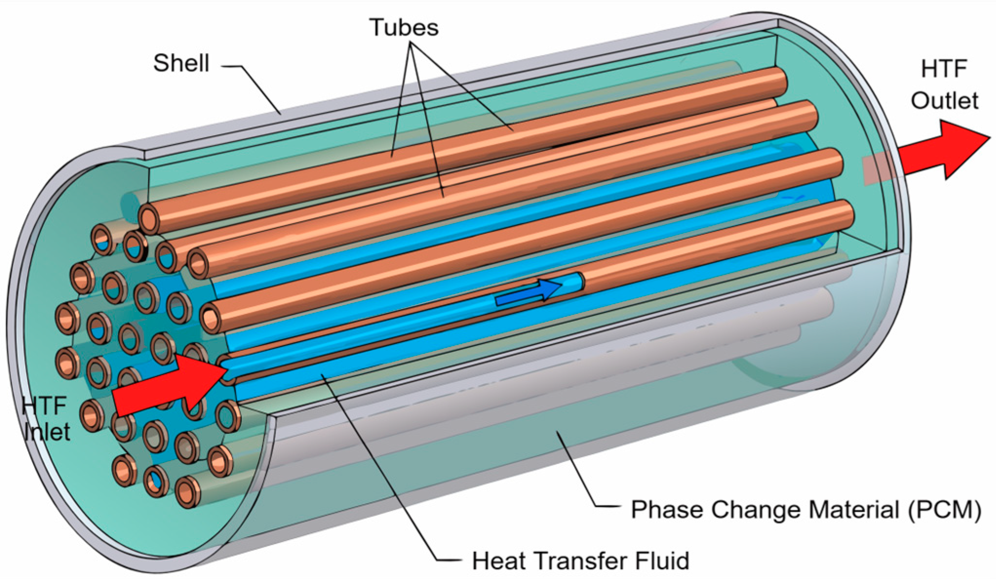
The standard shell-and-tube design for LHS systems consists of PCM occupying the shell side, while heat transfer fluid (HTF) flows through internal tubes as shown in Figure 1. This configuration offers a practical balance between simplicity and scalability. However, its performance is limited by the inherently low thermal conductivity of PCM [20,21]. To address this limitation, multiple PCMs with different melting temperatures can be staged within the system, improving heat transfer uniformity. Studies have shown that using three cascaded PCM units enhances latent heat utilization and system effectiveness by approximately 15–20% compared to single-PCM systems [20]. Another widely adopted enhancement involves the integration of finned tubes, which increases the effective heat transfer surface area and accelerates the phase change process. Experimental results indicate that finned designs can reduce solidification time by 30–40%, significantly improving overall thermal performance [22].

2.1.2. Triplex-Tube (Triple-Tube) Systems

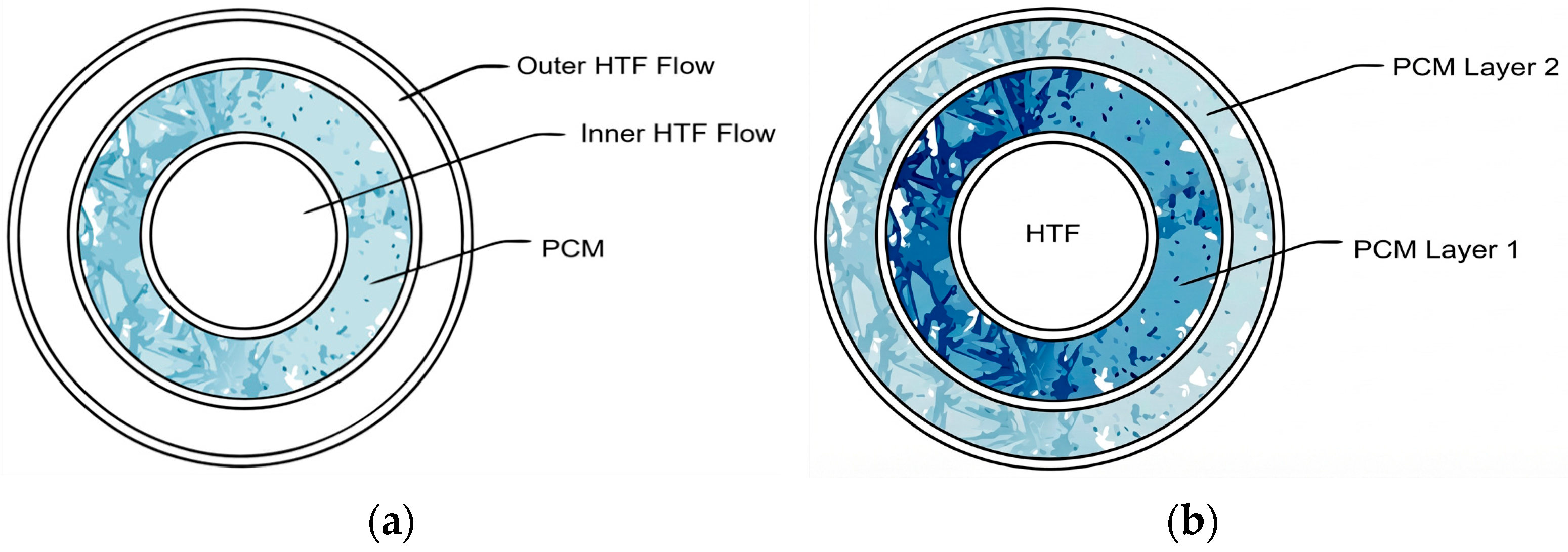
Triplex-tube heat exchangers (TTHEs) represent an advanced configuration for thermal energy storage systems. These designs employ concentric tubes, where the inner and outer tubes circulate heat transfer fluid (HTF), while the intermediate tube contains the PCM as shown in Figure 2a. This arrangement enables simultaneous heat storage and release along with direct hot water supply [23]. To enhance thermal performance, geometric optimization of the inner tube has been explored. Non-circular shapes such as square or pentagonal profiles showed significant improvement in heat transfer. For instance, square tubes have been shown to reduce solidification time by approximately 25% compared to conventional circular designs, primarily due to their increased surface area [24]. Furthermore, the incorporation of cascaded PCMs, as shown in Figure 2b, maintains a favorable thermal gradient throughout the system. This approach has demonstrated improvements in exergy efficiency ranging from 12% to 18% using materials such as RT35, RT50, and RT60 [25,26].

2.1.3. Double-Tube (Concentric Pipe) Systems

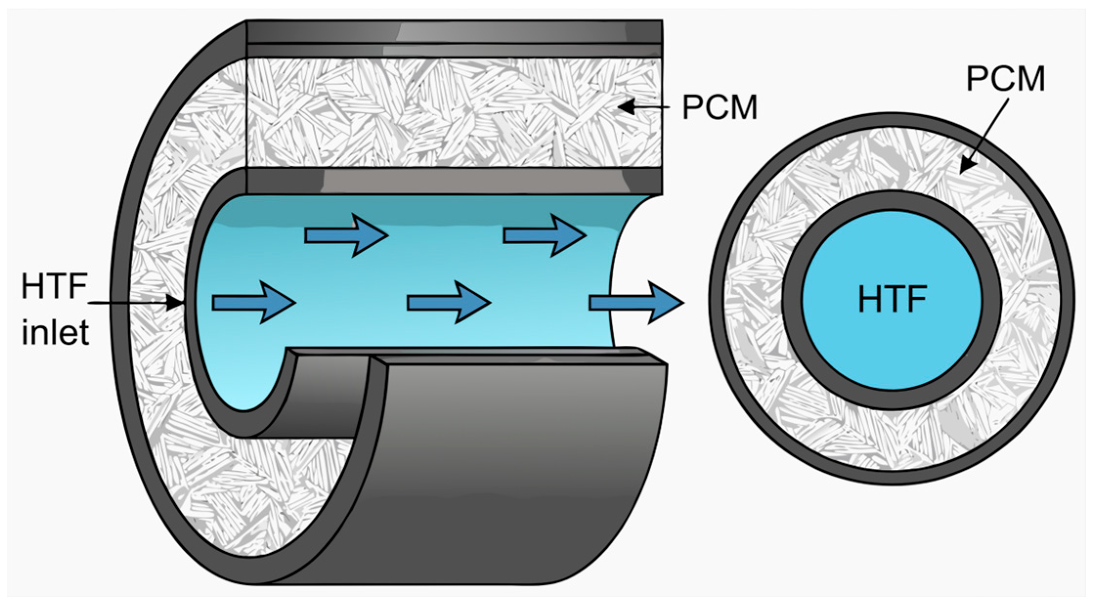
Double-tube configurations employ two concentric pipes with PCM typically surrounding an inner tube through which HTF flows, as shown in Figure 3. While more traditional than triplex-tube designs, these systems remain common for applications like domestic water heating and solar thermal systems [27].

2.1.4. Plate Heat Exchanger (PHE) Systems

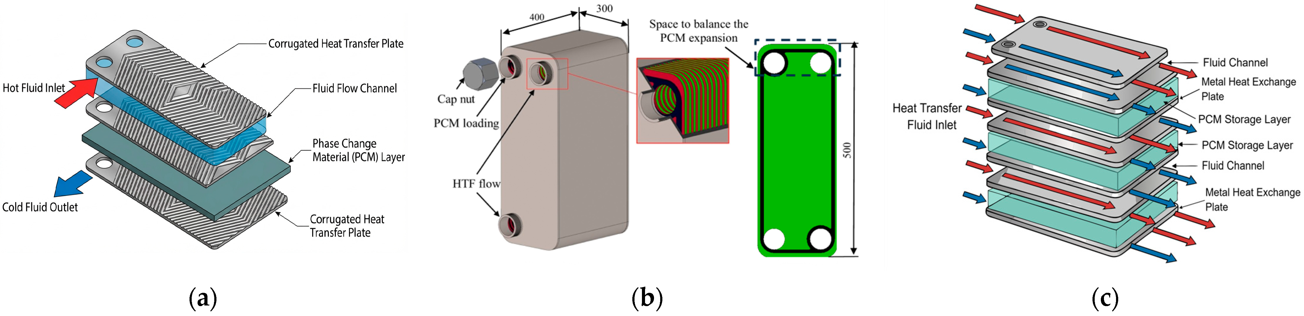
Plate-based configurations represent an alternative geometry where PCM is enclosed between parallel metal plates, with HTF flowing through channels. These systems offer a massive heat transfer surface within a compact design [28]. Variants include:

• Corrugated plate designs (Figure 4a): Using herringbone profiles for enhanced contact [29]
• Roll-bonded plate systems (Figure 4b): PCM is stored in a vessel and HTF flows through roll-bonded plates [28]
• Flat-plate configurations (Figure 4c): Simplified geometries with parallel HTF channels separated by PCM volumes [30]

2.1.5. Packed-Bed Systems

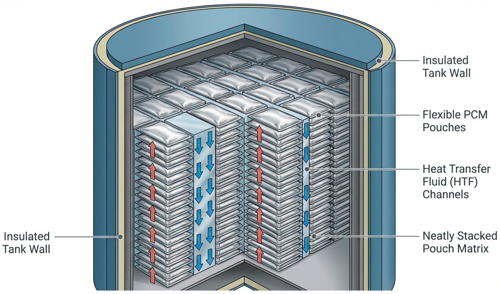
These configurations store PCM in encapsulated forms randomly packed within a tank, as shown in Figure 5, with HTF flowing through the bed. The advantage is increased heat transfer area through capsule encapsulation [31]. Modern variants include systems with ordered arrangements to control HTF flow distribution and improve performance uniformity [31].

The diversity of configurations illustrated above—shell-and-tube, triplex-tube, plate, and encapsulated systems—shares a common underlying physics: transient heat transfer with solid–liquid phase change. Understanding this physics is essential for appreciating why reduced-order modeling is both necessary and challenging. The following subsection presents the governing equations that describe these systems and the numerical methods used to solve them at full order, providing the foundation for the ROM techniques surveyed in Section 3.

2.2. Physical and Numerical Modeling of PCM-Based LHS System

Reduced-order modeling of LHS systems is fundamentally grounded in the mathematical and numerical description of phase change heat transfer. Most ROMs reported in the literature are derived from, trained on, or validated against high-fidelity numerical simulations that resolve transient melting and solidification processes of PCMs. A brief discussion of the governing equations and numerical solution strategies commonly employed in PCM-based LHS modeling are presented in the following subsections to contextualize the structure, complexity, and limitations of existing ROM approaches.

2.2.1. Governing Equations for Phase Change Heat Transfer

The thermal behavior of PCM-based LHS systems is primarily governed by the conservation of energy, with phase change introducing strong nonlinearities through latent heat effects. For most engineering applications, the energy equation is expressed in an enthalpy-based form, which allows both sensible and latent heat contributions to be treated within a unified framework [11,32].

In the absence of volumetric heat generation, the transient energy equation for a PCM domain can be written as

$$\rho {\displaystyle \frac{\partial h}{\partial t}}+\rho \mathbf{u}\cdot \nabla h=\nabla \cdot \left(k\nabla T\right),$$

(1)

where $\rho$ is the density, $h$ is the specific enthalpy, $\mathbf{u}$ is the velocity vector, $k$ is the thermal conductivity, and $T$ is the temperature. In purely conductive PCM systems, the convective term vanishes ($\mathbf{u}=0$), while in convection-enhanced systems, the energy equation is coupled with the momentum equations.

The enthalpy–temperature relationship accounts for latent heat storage through the introduction of a liquid-phase fraction $f_l$, commonly expressed as

$$h=c_{p}T+f_{l}L,$$

(2)

where $c_p$ is the specific heat capacity and $L$ is the latent heat of fusion. The liquid fraction varies between zero and unity and is typically defined as a function of temperature over a finite melting interval to ensure numerical stability [15].

The nonlinear coupling between temperature and phase fraction introduces a moving solid–liquid interface, which is the defining feature of PCM-based LHS systems. This nonlinearity significantly increases the dimensionality and stiffness of the resulting discretized system and poses a major challenge for reduced-order modeling.

In configurations where natural or forced convection within the molten PCM is important, the energy equation is coupled with the incompressible Navier–Stokes equations through buoyancy-driven flow, often modeled using the Boussinesq approximation [33]. However, many ROM studies focus on conduction-dominated configurations or treat convective effects in a simplified manner to reduce computational complexity.

2.2.2. Numerical Methods for High-Fidelity PCM Simulations

Several numerical methods have been developed to solve the governing equations of phase change heat transfer. Among these, the enthalpy–porosity method is the most widely used approach for simulating melting and solidification in PCM-based LHS systems [15,34]. In this method, PCM is treated as a porous medium in the mushy zone, with the liquid fraction acting as a porosity parameter that controls momentum damping in the partially molten region. This approach eliminates the need for explicit interface tracking and is therefore well suited for complex geometries.

An alternative formulation is the effective heat capacity method, in which the latent heat is incorporated into an augmented heat capacity over the phase change temperature range [16]. While computationally attractive, this method may suffer from numerical diffusion and reduced accuracy when sharp phase fronts are present.

High-fidelity PCM simulations are commonly discretized using the finite volume or finite element methods, combined with implicit time integration schemes to ensure numerical stability during rapid phase transitions [35]. Accurate resolution of steep temperature gradients near the phase interface typically requires fine spatial discretization, leading to large-scale systems of algebraic equations. As a result, transient simulations of charging and discharging cycles are computationally expensive, especially when multiple operating conditions or geometric parameters are considered.

From a reduced-order modeling standpoint, these numerical formulations give rise to FOMs characterized by:

• high state dimensionality,
• strong nonlinearities due to phase change,
• long transient simulation horizons,
• sensitivity to operating and geometric parameters.

These features directly influence the design and performance of ROM techniques applied to PCM-based LHS systems.

2.2.3. Implications for Model Order Reduction

The governing equations and numerical formulations described above pose several challenges for reduced-order modeling. First, the nonlinear enthalpy–temperature relationship, which arises directly from the governing energy and phase evolution formulations presented in Equations (1) and (2), and the presence of a moving phase boundary violate the linearity assumptions underlying classical projection-based ROMs, such as Proper Orthogonal Decomposition (POD)–Galerkin methods [36]. Consequently, a large number of modes may be required to accurately represent the system dynamics, particularly during rapid melting or solidification stages. Second, the strong dependence of PCM behavior on geometry, boundary conditions, and operating parameters limits the generalizability of ROMs trained for a specific configuration. This issue is particularly pronounced in finned or convection-enhanced LHS systems, where spatial complexity increases the effective dimensionality of the solution manifold. Finally, the multi-timescale and highly transient nature of PCM charging and discharging processes imposes stringent requirements on ROM stability and long-term accuracy. For applications such as real-time control, optimization, and digital twins, ROMs must remain robust across extended simulation horizons and varying operating conditions.

These features—high state dimensionality, strong nonlinearities, long transient horizons, and parameter sensitivity—directly influence ROM design. For example, the nonlinear enthalpy–temperature relationship violates the linearity assumptions underlying classical POD–Galerkin methods (Section 3.1.1), motivating nonlinear techniques such as the Discrete Empirical Interpolation Method (DEIM) (Section 3.2.1). Similarly, the dependence on geometry and boundary conditions limits the generalizability of data-driven surrogates (Section 3.3) trained for specific configurations. The multi-timescale behavior discussed in Section 4.2.3 imposes stringent requirements on ROM stability over extended simulation horizons, favoring methods that preserve long-term energy conservation.

3. Common Reduced-Order Modeling Methods

Reduced-order models (ROMs) are essential tools for simplifying complex, high-dimensional dynamical systems while preserving their essential characteristics, which is crucial for computational efficiency and analysis across various scientific and engineering disciplines [12,13,37]. The development of ROMs aims to bridge the gap between high-fidelity simulations, which can be computationally expensive and time-consuming, and the need for rapid analysis, optimization, and real-time control [13,14]. This is particularly relevant in fields like computational fluid dynamics (CFD), structural mechanics, and control systems [17,18]. The methodologies can be broadly categorized into projection-based linear ROMs. The following subsections detail each approach, with attention to their mathematical foundations, offline/online workflows, and inherent strengths and weaknesses.

3.1. Projection-Based Linear ROMs

Projection-based ROMs leverage linear subspaces to approximate system dynamics, relying on techniques like Proper Orthogonal Decomposition (POD) or a predefined basis.

3.1.1. Proper Orthogonal Decomposition (POD)–Galerkin

One of the most widely recognized and frequently applied techniques for model order reduction is Proper Orthogonal Decomposition (POD)–Galerkin [38,39,40,41,42,43,44,45]. POD–Galerkin constructs a reduced basis by extracting dominant spatial modes from high-fidelity simulation snapshots [19,46]. These modes, ranked by energy content, form an orthonormal basis that captures most system variance using far fewer vectors than the original full-order model [19]. The system’s governing equations (i.e., Equations (1) and (2)) are then projected onto this low-dimensional subspace using a Galerkin projection, leading to a reduced system of ordinary differential equations [46]. This projection preserves the physical structure of the original equations to some extent [47].

The mathematical basis of POD–Galerkin ROMs typically involves a structured workflow comprising offline and online phases [48,49]. In the offline phase, a set of snapshots (solutions from the FOM at different time instances or parameter values) is generated. POD is then applied to these snapshots to extract the dominant modes, which constitute the reduced basis. The FOM equations are projected onto this basis to derive the reduced-order system. In the online phase, the precomputed reduced-order system is solved rapidly for new parameters or time steps, yielding low-dimensional coefficients that are then mapped back to the high-dimensional physical space using the established POD modes [19,46].

POD–Galerkin ROMs are computationally efficient once the offline phase is complete, making them suitable for real-time applications and rapid parameter exploration [50]. They offer a physically consistent reduction, as the Galerkin projection maintains some connection to the underlying physics [47]. The method is particularly effective for systems with coherent structures or dominant modes [51]. Their performance can degrade significantly for highly nonlinear systems or systems with propagating fronts and shocks, as linear subspaces struggle to capture these features effectively [52]. The offline phase can be computationally expensive due to the need for FOM simulations and singular value decomposition (SVD) for POD basis generation [19]. Closure modeling is often required for nonlinear terms to account for the truncated modes’ influence, which can be complex [19,53].

3.1.2. Reduced Basis (RB)

The Reduced Basis method aims to construct a low-dimensional subspace that spans the solution manifold of a parametric partial differential equation (PDE) [54]. Unlike POD, which is purely data-driven, RB methods typically involve a greedy sampling approach to select basis vectors from a collection of solutions (snapshots) that are generated for different parameter instances [54,55]. The criterion for selecting snapshots often involves an a posteriori error estimator, ensuring that the chosen basis effectively approximates the solution across the entire parameter space. The FOM is then projected onto this basis [54].

The workflow of RB consists of offline and online phases. The offline stage involves a parameter space exploration. A series of FOM solutions are computed for various parameter values. A greedy algorithm iteratively selects parameter instances whose corresponding FOM solutions maximally enrich the reduced basis, typically guided by an error estimator. This process generates a compact, parameter-dependent reduced basis. In the online stage, for new parameter values, the precomputed reduced operators are used to solve the reduced-order system, providing a fast and accurate approximation of the FOM solution [54,55].

RB methods provide rigorous error bounds, which are crucial for certified real-time simulations and design optimization. They are well-suited for parametric PDEs, offering rapid evaluation for new parameter queries [54]. The greedy approach ensures an efficient and optimal basis selection [55].

Developing reliable and efficient error estimators can be challenging for complex problems, especially those with non-affine parameter dependencies [54]. Offline training can still be very time-consuming, particularly for high-dimensional parameter spaces [55]. Nonlinear problems often require hyper-reduction techniques to alleviate computational bottlenecks [47].

3.1.3. Proper Generalized Decomposition (PGD)

Proper Generalized Decomposition (PGD) is a model reduction technique that approximates high-dimensional solutions as a finite sum of separable functions, where each function is a product of univariate functions, typically one for each independent variable (e.g., spatial coordinates, time, and parameters) [56,57,58]. This separated representation drastically reduces the dimensionality of the problem by transforming a single high-dimensional problem into a series of coupled one-dimensional problems [59].

The offline phase of this method involves an iterative construction of the separable functions [56,57]. Starting with an initial guess, a fixed-point iteration or greedy algorithm computes one pair of functions (e.g., a spatial function and a parameter function) at a time, until a desired accuracy is reached [56]. This process is inherently “online” in the sense that once the separated representation is built, the solution for any combination of parameters or time can be evaluated directly without solving new systems [58].

PGD intrinsically handles high-dimensional parametric and multi-physical problems, often referred to as “curse of dimensionality” issues, by avoiding full tensor product spaces [56,58]. It produces a parameterized solution in a single offline computation, which can then be evaluated very rapidly for any parameter in the online phase [58]. PGD can also be applied to eigenvalue problems [59].

3.2. Nonlinear and Hyper-Reduced ROMs

The projection-based linear ROMs discussed in Section 3.1, while powerful, face fundamental limitations when applied to strongly nonlinear governing equations such as those of PCM phase change (see Section 2.2). Their computational efficiency is eroded because evaluating nonlinear terms (e.g., in the enthalpy–temperature relationship) still requires operations scaling with the high-dimensional FOM. To overcome this, hyper-reduction techniques such as the Discrete Empirical Interpolation Method (DEIM) and Gauss–Newton with Approximated Tensors (GNATs) have been developed. These methods approximate nonlinear terms by evaluating them only at a strategically selected subset of points, thereby preserving the speed advantage of the ROM.

3.2.1. Discrete Empirical Interpolation Method (DEIM)

The Discrete Empirical Interpolation Method (DEIM) is a hyper-reduction technique used to efficiently approximate nonlinear terms in projection-based ROMs, typically in conjunction with POD–Galerkin or RB methods [52,60]. The core idea is to approximate a high-dimensional nonlinear function using a small subset of its components (or “magic points”) and a corresponding empirical basis [61]. This avoids evaluating the nonlinear term over the entire high-dimensional domain, significantly reducing computational cost [60].

In the offline stage of this method, snapshots of the nonlinear term are collected, and an empirical basis for this term is constructed. DEIM then identifies a subset of “magic points” (spatial locations) where the nonlinear term needs to be evaluated. An interpolation matrix is also constructed. In the online stage, only the values of the nonlinear term at these magic points are computed, and the full nonlinear term is approximated using the precomputed empirical basis and interpolation matrix [60,62].

DEIM effectively alleviates the computational burden associated with nonlinear terms in ROMs, making projection-based ROMs feasible for many nonlinear problems [60,63]. It provides a systematic way to select sparse sensor locations [64].

The accuracy of DEIM depends heavily on the choice of magic points and the quality of the empirical basis, which can be sensitive to the problem’s characteristics [60,61]. The offline phase to construct the DEIM basis and select magic points can still be costly [64].

3.2.2. Gauss–Newton with Approximated Tensors (GNATs)

Gauss–Newton with Approximated Tensors (GNATs) is another hyper-reduction technique specifically designed to accelerate the solution of nonlinear reduced-order systems. It leverages the Gauss–Newton method for solving the nonlinear system, but crucially, it approximates the Jacobian and residual tensors by interpolating them at a reduced set of “collocation points” rather than computing them over the entire domain [65]. This approach is often combined with POD for basis generation [63].

The offline phase involves generating snapshots and constructing a POD basis for the solution. Additionally, snapshots of the nonlinear residual and its Jacobian are used to form reduced bases for these quantities. GNAT then identifies a set of optimal collocation points, similar to DEIM, where the nonlinear residual and Jacobian components are evaluated [63,65]. In the online phase, the nonlinear reduced-order system is solved using an iterative Gauss–Newton scheme, where the residual and Jacobian are approximated by evaluating them only at the pre-selected collocation points, leading to significant speed-ups [65].

GNAT is highly effective in accelerating nonlinear ROMs, offering significant computational savings compared to full-order Gauss–Newton iterations [63,65]. It maintains good accuracy by directly approximating the terms relevant to the nonlinear solver. GNAT can be embedded into hybrid snapshot simulations to improve efficiency and representation [65]. Like DEIM, the selection of optimal collocation points can be challenging and problem-dependent [65]. The method’s effectiveness relies on the smoothness of the nonlinear term and its Jacobian. The offline cost for constructing the GNAT basis and points can be substantial [63].

3.2.3. Adaptive Basis Methods

Adaptive basis methods aim to dynamically update or refine the reduced basis during the simulation or parameter exploration to better capture changing solution features, such as moving discontinuities, shocks, or localized phenomena [49,66]. This contrasts with static basis methods like standard POD–Galerkin, where the basis is fixed after the offline stage [66]. Techniques can include incremental POD (iPOD) or local bases defined over subdomains or specific parameter ranges [67].

The workflow often involves an iterative process where the solution is computed, an error indicator is evaluated, and if the error exceeds a threshold, the basis is enriched or adapted [67]. This might mean adding new modes, refining existing ones, or constructing entirely new local bases. For instance, some methods construct adaptive reduced bases using neural networks in the offline stage. The online phase then utilizes this adaptive basis, potentially switching between different local bases or updating the global basis as needed [49].

Adaptive basis methods are particularly effective for problems with complex, evolving dynamics or localized features that are difficult to capture with a single, static global basis [66]. They can significantly improve accuracy for systems where the solution manifold changes drastically [49]. The overhead associated with adaptivity, such as error estimation and basis enrichment, can increase computational cost, sometimes diminishing the benefits of reduction [67]. Designing robust and efficient adaptation strategies and error indicators is a complex task. Managing multiple local bases or dynamically updating a global basis adds complexity to the ROM formulation [49].

3.3. Data-Driven and Machine Learning ROMs

The ROM methodologies discussed in Section 3.1 and Section 3.2 are fundamentally physics-intrusive. They require explicit access to and manipulation of the governing equations to construct the ROM through projection or specialized nonlinear approximations. While powerful, this intrusion can be a barrier when high-fidelity simulations are proprietary or overly complex, or when the underlying physics is not fully organized in a tractable PDE form. This limitation has spurred the development of a parallel paradigm: data-driven and machine learning (ML) ROMs. These approaches operate in a non-intrusive manner, treating the high-fidelity model (or experimental system) as a “black box” that generates input–output data. Instead of projecting equations, they employ statistical learning and pattern recognition to construct a direct mapping from system parameters and inputs to the quantities of interest (e.g., temperature fields, phase front location, global heat rate).

3.3.1. Dynamic Mode Decomposition (DMD)

Dynamic Mode Decomposition (DMD) is a data-driven technique that extracts dynamically coherent structures (modes) from time-series data of a dynamical system [68,69]. It approximates the Koopman operator, a linear operator that governs the evolution of observables in a linear fashion, even for nonlinear systems [68,70]. DMD decomposes a sequence of snapshots into a set of modes, each associated with a fixed oscillation frequency and decay/growth rate. This allows for a low-rank, linear representation of potentially nonlinear dynamics [70].

In the offline phase, a sequence of snapshots from the FOM (or experimental data) is collected. DMD then constructs a low-rank linear surrogate model by identifying the dynamic modes and their corresponding eigenvalues that best describe the temporal evolution of the system [68,70]. In the online phase, this linear model is used to predict the future state of the system efficiently, often for various parameter settings, either by propagating the modes or by constructing a reduced-order basis for interpolation [71,72]. Online DMD methods can update the approximation as new data becomes available, making them suitable for streaming datasets [72,73].

DMD is entirely data-driven and “equation-free,” requiring no explicit knowledge of the governing equations [70,73]. It provides a linear, interpretable model of complex system dynamics, even for nonlinear systems. Online DMD variants are suitable for real-time applications and streaming data, allowing for dynamic updates to the ROM [72,73]. DMD’s performance can be sensitive to noise in the data and the choice of measurement functions [70]. It often struggles with systems exhibiting strong transient behaviors or highly complex, non-periodic dynamics [74]. The interpretability can decrease for highly complex systems where a large number of modes might be required [68]. When combined with POD and Polynomial Chaos Expansion (PCE), it can construct non-intrusive ROMs for time-dependent stochastic PDEs [75].

3.3.2. Neural Network ROMs

Neural Networks (NNs) offer a powerful way to learn complex, nonlinear mappings between high-dimensional inputs and low-dimensional outputs, or to directly approximate the dynamics of a reduced system [49,69,76]. They can act as surrogate models, learning the input–output relationships of a system, or as components within projection-based ROMs, providing closures or approximating specific nonlinear terms [53]. For instance, a neural network can construct adaptive reduced bases for transport problems [49]. Another application is in physics-informed neural networks (PINNs), where NNs are used within POD–Galerkin ROMs for solving inverse problems [46]. Transformer neural networks can also be used to extract temporal feature relationships from low-dimensional features derived from POD [77].

In the offline phase, a vast amount of high-fidelity data (input parameters, system states, time evolution) is used to train the neural network [49,76]. The NN learns the underlying relationships and builds a compact representation or a predictive model. This training process can be computationally intensive and requires careful hyperparameter tuning [49]. In the online phase, the trained NN quickly predicts system responses for new inputs, offering significant speed-ups compared to FOM simulations [76].

NNs are highly flexible and can approximate complex nonlinear relationships effectively, surpassing the limitations of linear ROMs for many challenging problems [69,76]. They are non-intrusive, meaning they do not require direct modification of the FOM code [50,77]. NNs can be used to construct adaptive bases [49] and learn closure terms for projection-based ROMs, improving their stability and accuracy [53]. Training NNs requires large datasets, which can necessitate extensive FOM simulations in the offline phase [53,76]. They are often considered “black-box” models, lacking the interpretability of physics-based ROMs [69]. Generalization to unseen parameter regimes or extreme conditions can be a challenge, and ensuring physical consistency is an active research area [47].

3.3.3. Autoencoders

Autoencoders are a type of neural network specifically designed for dimensionality reduction [69,78]. They consist of an encoder that maps high-dimensional input data to a low-dimensional latent space (the “bottleneck” layer) and a decoder that reconstructs the original data from this latent representation [79]. By minimizing the reconstruction error, the autoencoder learns an optimal nonlinear manifold embedding, effectively creating a nonlinear reduced basis [69].

In the offline phase, a dataset of FOM snapshots is fed into the autoencoder [79]. The network is trained to compress the data into a low-dimensional latent space and then decompress it back to the original high-dimensional space with minimal loss. This training process captures the essential features of the system’s states in the latent variables [78]. In the online phase, new high-dimensional inputs are passed through the trained encoder to quickly obtain their low-dimensional representation in the latent space. Subsequent simulations or analyses can be performed in this reduced space, and the decoder can reconstruct the full-order solution when needed. VpROM, for example, is a variational autoencoder-boosted ROM that defines a generalizable mapping for parametric dependencies in nonlinear systems [79]. Compressed neural networks using pruning and singular value decomposition can further reduce the storage requirements of autoencoders [80].

Autoencoders are powerful for nonlinear dimensionality reduction, capable of discovering optimal nonlinear embeddings for complex data [69,79]. They can capture intricate features that linear methods like POD might miss. The latent space provides a compact and efficient representation of the system state [78]. Similar to other NNs, autoencoders require extensive training data and can be computationally expensive to train [79]. Their black-box nature can hinder physical interpretability and guarantee of physical consistency. The choice of autoencoder architecture and hyperparameters significantly impacts performance [78]. Compared to POD and DMD, autoencoders can have larger storage requirements, though compression techniques exist to mitigate this [80].

3.3.4. Gaussian Process ROMs

Gaussian Process (GP) models are non-parametric, Bayesian approaches to regression and function approximation. When applied to ROMs, GPs can model the relationship between system parameters and reduced-order coefficients or directly approximate the system’s response in the reduced space. They provide not only predictions but also a measure of uncertainty (variance) associated with those predictions, which is a key advantage [69].

In the offline phase, a sparse set of FOM solutions (snapshots) for various parameter values is used to train the GP model. The GP learns the mapping from parameters to the reduced solution space, typically involving the definition of a covariance function (kernel) that encodes assumptions about the smoothness and correlation of the function being approximated. In the online phase, for new parameter inputs, the trained GP can rapidly predict the corresponding reduced-order solution, along with an associated uncertainty quantification, without requiring additional FOM evaluations [69].

GPs provide inherent uncertainty quantification, which is crucial for applications like robust design and risk assessment. They are highly flexible and can model complex, nonlinear relationships with relatively small datasets compared to deep neural networks [69]. GPs can be particularly effective for exploring parameter spaces where FOM evaluations are costly. The computational cost of GP inference scales cubically with the number of training data points, limiting their applicability to very large datasets. Choosing an appropriate kernel function is critical for performance and can be problem-dependent. They can sometimes struggle with very high-dimensional parameter spaces or problems with sharp discontinuities in the solution manifold [69].

3.4. Unified Mathematical Framework for ROMs

The ROM methodologies surveyed in Section 3.1, Section 3.2 and Section 3.3 can be understood within a unified mathematical framework that reveals their relationships and clarifies the placement of hybrid and physics-informed approaches. This framework links the full-order model (FOM) formulation to its reduced counterpart through a sequence of approximations.

3.4.1. Full-Order Model Formulation

Consider a parameterized PDE governing PCM-based LHS systems (from Section 2.2):

$${\displaystyle \frac{\partial u}{\partial t}}+\mathcal{N}(u;\mu )=0,u(0)=u_0(\mu ),$$

(3)

where $u(\mathbf{x},t;\mu )\in \mathcal{V}$ is the solution field (temperature, velocity, pressure, phase fraction) in a high-dimensional Hilbert space $\mathcal{V}$ (dimension $N\sim {10}^5-{10}^7$ after discretization), $\mu \in \mathcal{P}\subset {\mathbb{R}}^d$ represents parameters (material properties, geometry, boundary conditions), and $\mathcal{N}$ is a nonlinear differential operator incorporating phase change physics (enthalpy–porosity, convection, conduction).

After spatial discretization (finite volume, finite element), we obtain a system of ODEs:

$$\mathbf{M}\left(\mu \right){\displaystyle \frac{d\mathbf{u}}{dt}}+\mathbf{A}\left(\mu \right)\mathbf{u}+\mathbf{F}\left(\mathbf{u};\mu \right)=0,\mathbf{u}\left(0\right)={\mathbf{u}}_0\left(\mu \right),$$

(4)

where $\mathbf{u}(t;\mu )\in {\mathbb{R}}^N$ is the discrete state vector, $\mathbf{M}$ is the mass matrix, $\mathbf{A}$ contains linear terms, and $\mathbf{F}$ represents nonlinear terms (enthalpy–temperature relationship, convective terms).

3.4.2. Reduction via Approximation in Low-Dimensional Space

All ROMs seek an approximation $\tilde{\mathbf{u}}\approx \mathbf{u}$ in a low-dimensional space of dimension $r\ll N$:

$$\tilde{\mathbf{u}}(t;\mu )=\mathbf{\Phi }\mathbf{a}(t;\mu )+\mathrm{possible} \mathrm{corrections},$$

(5)

where $\mathbf{\Phi }\in {\mathbb{R}}^{N\times r}$ is the reduced basis matrix (columns are basis vectors) and $\mathbf{a}(t;\mu )\in {\mathbb{R}}^r$ are reduced coefficients. The basis may be:

• Linear global basis: $\mathbf{\Phi }$ constant (POD, RB) (Section 3.1.1 and Section 3.1.2)
• Separated representations: $\mathbf{\Phi }={\mathbf{\Phi }}_1\otimes {\mathbf{\Phi }}_2\otimes \cdots$ (PGD) (Section 3.1.3)
• Adaptive basis: $\mathbf{\Phi }\left(t\right)$ evolving with solution (Section 3.2.3)
• Nonlinear manifold: $\tilde{\mathbf{u}}=\mathbf{\Psi }\left(\mathbf{z}\right)$ where $\mathbf{\Psi }$ is nonlinear (autoencoders) (Section 3.3.3)

3.4.3. Obtaining Reduced Dynamics

The evolution equations for reduced coefficients are obtained through one of three paradigms:

• Paradigm 1: Projection (Physics-Intrusive)

Substitute $\tilde{\mathbf{u}}=\mathbf{\Phi }\mathbf{a}$ into the governing equations and project onto the reduced space (typically Galerkin projection: multiply by ${\mathbf{\Phi }}^T$):

$${\mathbf{\Phi }}^T\mathbf{M}\mathbf{\Phi }{\displaystyle \frac{d\mathbf{a}}{dt}}+{\mathbf{\Phi }}^T\mathbf{A}\mathbf{\Phi }\mathbf{a}+{\mathbf{\Phi }}^T\mathbf{F}(\mathbf{\Phi }\mathbf{a};\mu )=0,$$

(6)

This yields a reduced system of dimension $r$:

$${\mathbf{M}}_r{\displaystyle \frac{d\mathbf{a}}{dt}}+{\mathbf{A}}_r\mathbf{a}+{\mathbf{\Phi }}^T\mathbf{F}(\mathbf{\Phi }\mathbf{a};\mu )=0,$$

(7)

The computational bottleneck is evaluating the nonlinear term ${\mathbf{\Phi }}^T\mathbf{F}(\mathbf{\Phi }\mathbf{a};\mu )$, which still scales with $N$. Hyper-reduction methods (DEIM, GNAT) [Section 3.2] approximate this term as:

$${\mathbf{\Phi }}^T\mathbf{F}(\mathbf{\Phi }\mathbf{a};\mu )\approx {\mathbf{\Phi }}^T{\mathbf{P}}^T\left(\mathbf{P}\mathbf{F}\right(\mathbf{\Phi }\mathbf{a};\mu \left)\right),$$

(8)

where $\mathbf{P}\in {\mathbb{R}}^{m\times N}$ selects $m\ll N$ sampling points where $\mathbf{F}$ is evaluated.

• Paradigm 2: Data-Driven System Identification (Non-Intrusive)

Instead of projecting equations, learn the reduced dynamics directly from data. Represent the evolution in reduced space as:

$${\displaystyle \frac{d\mathbf{a}}{dt}}=\mathcal{G}(\mathbf{a};\mu ),$$

(9)

where $\mathcal{G}$ is learned from trajectories $\left(\mathbf{a}\left(t_k\right),\dot{\mathbf{a}}\left(t_k\right)\right)$ extracted from FOM snapshots. Specific methods:

• DMD [Section 3.3.1]: Assumes linear dynamics $\dot{\mathbf{a}}=\mathbf{K}\mathbf{a}$, learning $\mathbf{K}$ from data
• Neural network ROMs [Section 3.3.2]: Represent $\mathcal{G}$ as a neural network trained on snapshot data
• Sparse identification (SINDy): Learn parsimonious nonlinear expressions for $\mathcal{G}$ (emerging approach)

• Paradigm 3: Direct Input–Output Mapping (Non-Intrusive)

Bypass state evolution entirely and learn direct mapping from inputs to quantities of interest:

$$\mathbf{y}(t;\mu )=\mathcal{H}(\mu ,t),$$

(10)

where $\mathbf{y}$ may be outlet temperature, heat transfer rate, or stored energy. Methods:

• Gaussian process regression [Section 3.3.4]: $\mathcal{H}$ as GP with kernel capturing input correlations
• Kriging metamodels [1]: Similar to GP, typically for steady or time-integrated outputs
• Neural network surrogates: $\mathcal{H}$ as a feedforward network mapping $\left(\mu ,t\right)$ to $\mathbf{y}$

3.4.4. Taxonomy of ROM Approaches

Based on the discussed framework above, ROMs can be classified along three axes as presented in

Table 1. Taxonomy of ROM approaches.

Axis	Categories	Methods
Basis construction	Linear global (static)	POD, RB
	Linear global (adaptive)	Adaptive POD, local bases
	Separated representations	PGD
	Nonlinear manifold	Autoencoders
Dynamics learning	Projection (intrusive)	POD–Galerkin, RB
	Data-driven identification	DMD, neural ODEs
	Direct mapping	Kriging, GP, feedforward NN
Nonlinear treatment	Full evaluation	Projection without hyper-reduction
	Hyper-reduction	DEIM, GNAT
	Learned approximation	Neural network closure models

.

3.4.5. Placement of Hybrid and Physics-Informed Methods

Hybrid and physics-informed methods combine elements from multiple paradigms:

• Physics-Informed Neural Networks (PINNs) [10,46] solve the inverse problem of finding parameters $\mu$ that make ROM predictions consistent with sparse observations while penalizing violation of governing equations. Mathematically:

$${\mathrm{m}\mathrm{i}\mathrm{n}}_{\mu }\parallel \tilde{\mathbf{u}}\left({\mathbf{x}}_{obs}\right)-{\mathbf{u}}_{obs}{\parallel }^2+\lambda \parallel \mathcal{R}(\tilde{\mathbf{u}};\mu ){\parallel }^2,$$

(11)

where $\mathcal{R}$ is the PDE residual. PINNs can be viewed as Paradigm 3 (direct mapping) with a physics-based regularization term.

ML-Augmented Projection ROMs [53] use projection (Paradigm 1) for resolved dynamics but learn closure terms representing truncated mode effects from data (Paradigm 2):

$${\mathbf{\Phi }}^T\mathbf{F}(\mathbf{\Phi }\mathbf{a};\mu )\approx \underset{\mathrm{projected} \mathrm{physics}}{\underbrace{{\mathbf{\Phi }}^T{\mathbf{F}}_{resolved}(\mathbf{\Phi }\mathbf{a};\mu )}}+\underset{\mathrm{ML} \mathrm{closure}}{\underbrace{\mathbf{G}(\mathbf{a};\mu ;\theta )}},$$

(12)

where $\mathbf{G}$ is a neural network trained on residual errors.

Grey-Box Models [1] combine simplified physics (Paradigm 1 with aggressive physical reduction, Section 3) with data-driven calibration (Paradigm 3):

$$\dot{\mathbf{a}}=\underset{\mathrm{simplified} \mathrm{physics}}{\underbrace{{\mathbf{f}}_{physics}(\mathbf{a};\mu )}}+\underset{\mathrm{data-driven} \mathrm{correction}}{\underbrace{{\mathbf{g}}_{calibration}(\mathbf{a};\mu ;\theta )}},$$

(13)

Physics-Constrained Neural Networks enforce hard constraints (energy conservation, bounds) through architecture design or constrained optimization, ensuring predictions satisfy physical laws even when trained on limited data.

3.5. Comparative Summary of Common ROM Methodologies

The spectrum of ROM techniques detailed in Section 3.1, Section 3.2 and Section 3.3 represents a continuum from rigorous, physics-intrusive projection methods to flexible, equation-free data-driven surrogates. Each category offers a distinct balance between fidelity to first principles, computational efficiency, and implementation complexity, making them differentially suited to specific stages of the LHS system lifecycle—from initial design exploration to real-time control and digital twinning.

Table 2. Summary of common ROM methodologies.

Characteristic	Projection-Based Linear ROMs	Nonlinear & Hyper-Reduced ROMs	Data-Driven & ML ROMs
Core Philosophy	Project governing equations onto a low-dimensional linear subspace.	Extend projection methods to handle nonlinearity via term approximation or basis adaptation.	Learn system behavior directly from data, bypassing explicit equation reduction.
Intrusiveness	Intrusive: Requires full access to and manipulation of FOM equations.	Intrusive: Requires access to FOM equations and nonlinear terms.	Non-Intrusive: Treats FOM as a black-box data generator.
Handling of PCM Nonlinearity	Poor. Linear subspaces struggle with moving boundaries and enthalpy jumps. Often requires many modes.	Good to Excellent. DEIM/GNAT approximate nonlinear terms; adaptive bases track evolving dynamics.	Excellent. ML models (NNs, GPs) are inherently flexible nonlinear function approximators.
Offline Cost & Complexity	High. Requires FOM snapshot generation and matrix decompositions (e.g., SVD).	Very High. Adds complex steps: nonlinear term snapshot generation, magic point selection, or basis adaptation logic.	Highest. Demands extensive FOM runs for training data and computationally intensive model training/tuning.
Online (Runtime) Performance	Very Fast. Solving a small ODE system.	Fast. Solving a small ODE system with pre-computed sparse evaluations.	Extremely Fast. Typically a simple forward pass through a trained model (e.g., NN).
Interpretability & Physical Consistency	High. Structure mirrors original physics; Galerkin projection ensures certain conservation properties.	Moderate to High. Physics-based core remains, but approximations reduce strict consistency.	Low (“Black-Box”). Internal logic is opaque; predictions may violate physical laws without constraints (e.g., PINNs).
Generalizability & Extrapolation	Moderate. Limited to parameter/state space sampled for basis generation.	Moderate. Similar to linear ROMs, but adaptive methods can improve within bounds.	Poor. Performance degrades rapidly outside the convex hull of the training data.
Best-Suited Applications	Linear subsystems, sensitivity analysis, problems with strong coherent structures.	High-fidelity control, digital twins where nonlinear physics must be retained with some efficiency.	Rapid design optimization, system-level simulation, complex geometries where intrusive reduction is infeasible.
Key Enabling Technology for PCM-based LHS	POD–Galerkin for conduction-dominated regimes; RB for parametric studies.	DEIM/GNAT for enthalpy–porosity models; adaptive bases for tracking phase fronts.	ANN/XGBoost surrogates for complex finned/triplex-tube systems; autoencoders for nonlinear field compression.

summarizes the characteristics of each ROM methodology.

Projection-Based Linear ROMs are the most interpretable and mathematically founded. They excel in systems where the dynamics are dominated by coherent structures that can be captured in a low-rank linear subspace. Their key strength lies in preserving a direct, albeit reduced, connection to the original governing equations, which aids in understanding and trust. However, their fundamental assumption of linearity is their primary weakness when applied to the strongly nonlinear, moving-boundary problems inherent in PCM phase change. While they can achieve significant speed-ups for linear or weakly nonlinear components, they often become inefficient or inaccurate for full charging/discharging cycles without augmentation.

Nonlinear and Hyper-Reduced ROMs evolved directly to address the core limitation of projection-based linear ROMs methods: handling system nonlinearity while maintaining an intrusive, physics-based structure. Techniques like DEIM and GNAT preserve the projection framework but introduce sophisticated approximations (e.g., sparse sampling of nonlinear terms) to recover computational efficiency. Adaptive basis methods further enhance flexibility by allowing the reduced subspace to evolve with the solution. These methods represent a powerful compromise, offering improved nonlinear capability while retaining more interpretability than purely data-driven models. Their trade-off is increased algorithmic and implementation complexity in the offline stage.

Data-Driven and Machine Learning ROMs represent a paradigm shift. They forgo the explicit projection of equations in favor of learning input–output relationships or low-dimensional embeddings directly from data. This non-intrusive nature is their greatest asset, allowing for integration with complex or proprietary FOMs and providing extreme flexibility in modeling nonlinear and even non-physical correlations. They have demonstrated remarkable speed-ups for complex geometries (e.g., finned enclosures). Their principal liabilities are the “black-box” nature, which complicates physical interpretation and validation; a high demand for comprehensive, high-quality training data; and a general lack of built-in guarantees for physical consistency or extrapolation robustness.

The choice among these methods is not a question of which is universally superior, but which is most fit-for-purpose given the application’s requirements for accuracy, speed, interpretability, and available resources (data, FOM access, expertise). Table 1 provides a concise comparison of the three primary ROM categories across key attributes relevant to PCM-based LHS system modeling. With this methodological foundation established, Section 4 examines why these ROM techniques are particularly valuable—and challenging—for PCM-based LHS applications.

4. Applicability of ROMs to PCM-Based Latent Heat Storage Systems

ROMs are essential for efficiently simulating complex thermal systems, particularly in the context of PCM-based latent heat storage systems [2,9,81]. These systems exhibit high energy density and isothermal storage capabilities, making them attractive for various applications, including solar engineering, building heating and cooling, and thermal management of electronic devices [11,82,83,84]. However, the detailed simulation of PCM systems, which involves phase change, conduction, and convection, can be computationally intensive, necessitating the use of ROMs to reduce computational cost while maintaining sufficient accuracy [9,13,85]. ROMs are particularly applicable to PCM-based LHS systems because they can capture the dominant thermal dynamics without the need for detailed spatial discretization at every time step [86,87].

4.1. Advantages of ROMs in Latent Heat Storage Systems

ROMs enable faster iteration cycles during the design phase of PCM-based TES systems. Engineers can quickly evaluate different PCM types, encapsulation methods, or heat exchanger geometries to optimize performance. For instance, a ROM of encapsulated PCMs can be used to study the effects of porosity, capsule diameter, and heat transfer fluid (HTF) flow rate on overall system performance [81]. Studies have developed approximation-assisted reduced-order PCM heat exchanger models to speed up the design process of thermal energy storage devices [1].

For effective operation and control of LHS systems, particularly in applications like building-integrated TES, real-time feedback is crucial [88,89]. ROMs can provide rapid predictions of the system’s thermal state, enabling proactive control strategies for charging and discharging cycles [90]. This is vital for managing the intermittent nature of renewable energy sources, such as solar or wind power, by balancing energy supply and demand.

Predicting the thermal response of a PCM system and estimating its state-of-charge (SOC) is challenging due to the nonlinearity introduced by phase change [85]. ROMs, especially those validated against experimental data, can accurately predict transient thermal output and SOC, crucial for efficient energy management [91]. A 1D ROM, for example, has been developed for a novel latent thermal energy storage system addressing challenges like low thermal conductivity and expensive encapsulation processes [2].

PCMs often suffer from low thermal conductivity and potential leakage during phase transitions. Strategies to mitigate these issues include microencapsulation or the addition of highly conductive filler materials [92,93,94]. ROMs can effectively model the enhanced heat transfer in these composite materials. Different types of PCMs, including organic (e.g., paraffin), inorganic (e.g., salt hydrates), and eutectic mixtures, have varying thermal properties and operating temperature ranges. These can be categorized by their melting temperatures, from low-temperature PCMs like ice and water gel to high-temperature PCMs such as molten salts and metal alloys [95]. The selection of appropriate PCM depends on the application, ranging from transient thermal management of electronic devices, where rapid heat absorption is needed, to seasonal thermal energy storage (STES) for long-term energy balancing [96,97]. ROMs can aid in understanding how different PCM characteristics influence overall system performance across these diverse applications.

4.2. Core Challenges in PCM-Based LHS Modeling

While ROMs offer significant benefits, their development and deployment in PCM-based latent heat storage (LHS) systems are accompanied by notable challenges. It is complicated by four interconnected physical phenomena, each introducing distinct modeling difficulties [98,99].

4.2.1. Latent Heat Nonlinearity

The dominant source of nonlinearity originates from the phase change process itself [100,101,102]. During melting and solidification, PCMs exhibit highly nonlinear thermophysical behavior: the enthalpy–temperature relationship becomes strongly nonlinear in the phase transition region, and key properties—specific heat, thermal conductivity, and density—vary substantially between solid and liquid phases [103]. This nonlinearity is compounded by buoyancy-driven natural convection in the molten phase, which creates spatially nonuniform temperature and velocity fields that depend on local thermal gradients and geometry [104,105]. Hysteresis between melting and solidification further complicates prediction, as the material’s thermal history influences its response [98]. Together, these nonlinear effects mean that linear modeling approaches fundamentally cannot capture PCM dynamics, necessitating either nonlinear projection methods (Section 3.2) or flexible data-driven surrogates (Section 3.3).

While the enthalpy–temperature nonlinearity poses significant challenges, it is important to acknowledge that the solution of the Navier–Stokes equations for natural or forced convection in the liquid phase represents an even more formidable computational task. The coupled momentum and energy equations introduce additional nonlinearities through the convective term $\left(\mathbf{u}\cdot \nabla \right)\mathbf{u}$ and the Boussinesq coupling between temperature and buoyancy forces. Resolving boundary layers and recirculating flows in the liquid PCM requires fine spatial discretization and small time steps, dramatically increasing full-order model cost. Many ROMs avoid this complexity by either: (a) neglecting convection entirely (pure conduction assumption), justified for small capsules [81] or high-viscosity PCMs where $Ra<{10}^3$; (b) lumping convection effects into enhanced effective conductivity [9]; or (c) retaining simplified convection models (e.g., 2D axisymmetric with Boussinesq approximation [8]) that reduce but do not eliminate the computational burden. When convection is neglected, this simplification must be explicitly justified with reference to Rayleigh number, geometry dimensions, and expected flow regimes, as its omission can lead to substantial underprediction of heat transfer rates—particularly during later stages of melting when liquid regions are large [105,106].

4.2.2. Moving Phase Boundaries

The solid–liquid interface propagates dynamically through the material, forming a boundary that is inherently time-dependent and unknown a priori [107,108,109]. This moving-boundary problem—classically known as the Stefan problem—requires simultaneous solution for temperature fields and interface position [110]. Fixed-grid methods like enthalpy–porosity avoid explicit interface tracking but introduce numerical challenges: fine spatial discretization is needed to resolve the phase front, and non-physical behavior can arise in close-contact melting scenarios where velocity errors exceed 50% [111]. Density changes between phases cause volumetric expansion or contraction as the interface advances, further complicating energy balances [112]. From a ROM perspective, moving boundaries mean that the solution’s dominant spatial features evolve, challenging static basis assumptions and motivating adaptive methods (Section 3.2.3).

4.2.3. Multi-Timescale Dynamics

PCM systems inherently exhibit dynamics spanning multiple timescales [113]. Latent heat absorption or release occurs rapidly over short intervals, while conduction in solid phases and convection in liquid phases evolve more gradually. Cascaded latent heat storage systems compound this complexity, as individual PCM layers may undergo phase change asynchronously [114]. The dynamic response can span from sub-millisecond thermal transients to charging/discharging processes lasting hours [115]. This wide range challenges variable time-step solvers, which often encounter convergence difficulties during rapid phase change events [116]. For ROMs, multi-timescale behavior demands that reduced bases capture both fast and slow modes; projection-based methods may require many modes to represent the full temporal spectrum, while data-driven methods need training data that adequately samples all relevant timescales.

4.2.4. Geometry and Boundary Sensitivity

Performance is strongly influenced by both geometric configuration and imposed boundary conditions [117,118,119]. The shape, orientation, and aspect ratio of the PCM enclosure affect heat transfer pathways, natural convection development, and phase change uniformity [106,120]. Enhancement techniques—fins, metal foams, and encapsulation—further increase geometric complexity and parameter sensitivity [100,121,122]. Boundary conditions (constant temperature, constant heat flux, cyclic operation) directly determine charging/discharging behavior and must be accurately represented in ROMs [123,124]. This sensitivity means that ROMs trained for one configuration rarely generalize to others; each geometry or boundary condition change typically requires new training data or basis construction, limiting transferability.

The four interconnected physical challenges inherent to PCM-based LHS systems—latent heat nonlinearity, moving phase boundaries, multi-timescale dynamics, and geometry/boundary sensitivity—establish the key phenomena that any reduced-order model must adequately represent.

Table 3. Physical challenges and best-suited ROM approaches.

Physical Challenge	ROM Development Impact	Best-Suited ROM Approaches	Reasoning	Representative Studies
Latent heat nonlinearity	Linear subspaces (POD) require many modes; nonlinear term evaluation costly	DEIM/GNAT; Neural networks; Gaussian processes	Hyper-reduction methods approximate nonlinear terms efficiently; ML methods inherently handle nonlinear mappings	DEIM [60,61]; ANN [125]; XGBoost [126]
Moving phase boundaries	Static bases fail as dominant spatial features evolve	Adaptive basis methods; POD with extensive snapshot libraries; CFD look-up tables	Adaptive methods track evolving fronts; look-up tables precompute interface dynamics offline	Adaptive POD [49]; CFD look-up [9]; POD interpolation [8]
Multi-timescale dynamics	ROM must capture both fast and slow modes; training data must sample all scales	POD with sufficient modes; Hybrid (ε-NTU + data); Physics-based with timescale separation	POD captures spectral content; grey-box models separate fast (phase change) and slow (sensible) periods	POD [8]; ε-NTU grey-box [1]; two-temperature [81]
Geometry/boundary sensitivity	ROMs trained for one configuration rarely generalize	ML-based surrogates (with geometric parameters as inputs); Parametric POD; Autoencoders	ML methods can include geometry parameters; autoencoders learn nonlinear geometric embeddings	ANN [125]; XGBoost [126]; Autoencoders [79]

explicitly links each of these challenges to the ROM methodologies best suited to address them, based on the capabilities surveyed in Section 3 and the case study evidence presented in Section 5. This explicit mapping between physical challenges and methodological capabilities provides a theoretical foundation for the practical decision framework developed in Section 5.9. By mapping the impact of each challenge on ROM development (e.g., the need for nonlinear term approximation, adaptive bases, or parameter-space sampling) to concrete methodological families—ranging from physics-intrusive projection methods that preserve governing equation structure to purely data-driven surrogates that learn behavior directly from simulation data—this table provides a theoretical foundation for understanding why certain approaches excel in specific contexts. With this framework in place, Section 5 transitions from examining common methodological characteristics to analyzing individual application cases, demonstrating how the techniques catalogued in Section 3 have been tailored to address the core challenges for particular system geometries and operating conditions. The selected cases span the full spectrum of method classifications introduced earlier while illustrating how the physical complexities of PCM modeling manifest in practice.

5. ROMs for PCM-Based Latent Heat Storage Systems

The development of ROMs for LHS systems has evolved along several methodological trajectories, each balancing computational efficiency against physical fidelity. Current approaches range from physics-based analytical models to data-driven machine learning techniques, with hybrid methods combining the strengths of both paradigms [9]. This section examines studies representing the state-of-the-art in ROM development for LHS systems, reporting their LHS configuration and physical scope, governing physics incorporated into the ROM, the chosen ROM methodology and model class, snapshot or training strategy, model order and associated computational cost, accuracy metrics and validation approach, intended application and use case, as well as reported limitations.

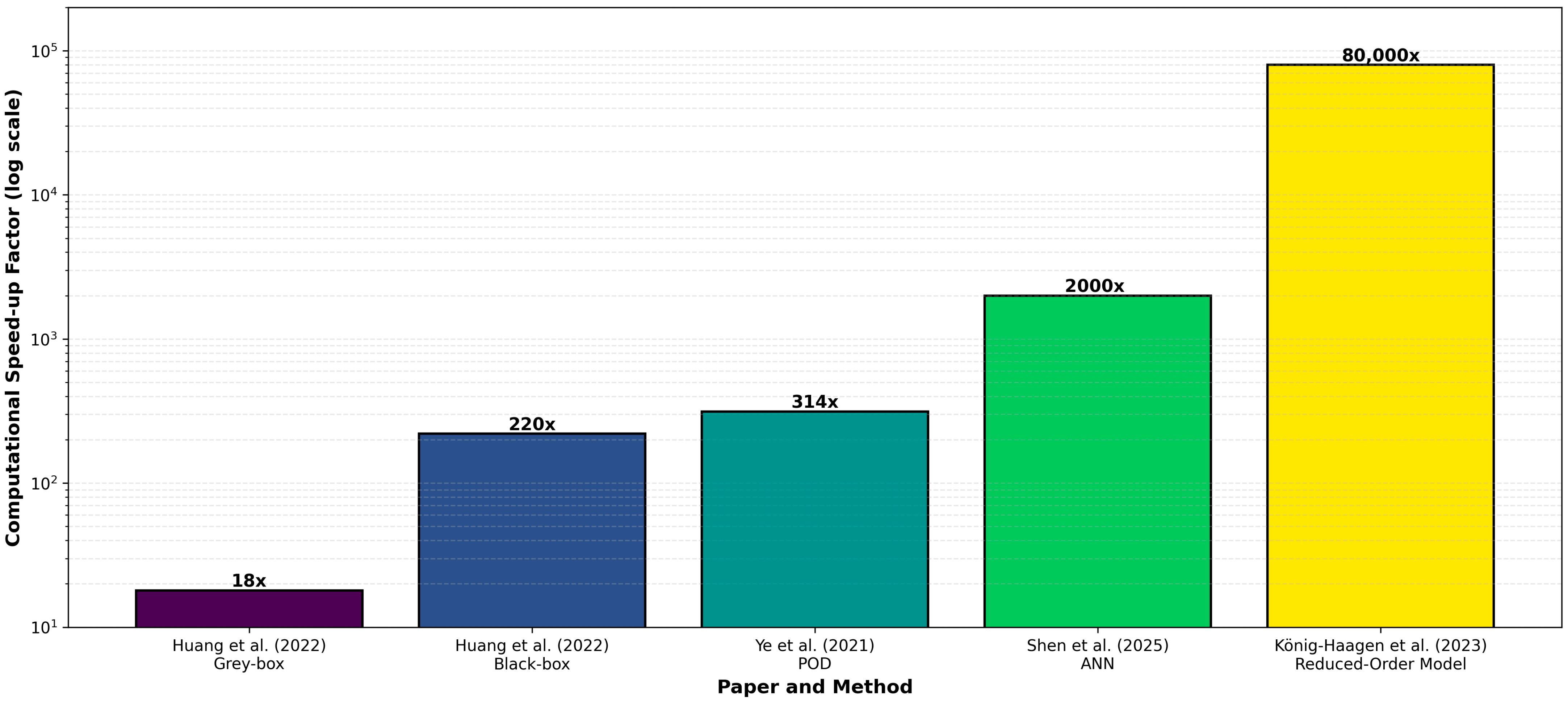
The seven case studies examined in this section were selected through a systematic literature screening process designed to balance depth of analysis with representative coverage of the ROM landscape. From an initial corpus of over 40 relevant publications identified through Scopus and Web of Science searches using keywords (‘reduced-order model,’ ‘PCM,’ ‘latent heat storage,’ ‘proper orthogonal decomposition,’ ‘machine learning’), studies were included in the detailed analysis if they satisfied three criteria: (1) methodological completeness—the study must provide sufficient detail on ROM construction, training data generation, and validation approach to enable critical evaluation; (2) diversity of representation—the selected studies collectively span the major ROM categories identified in Section 3 (physics-based, projection-based, hybrid, and data-driven), ensuring coverage of the full methodological spectrum; and (3) performance quantification—the study must report quantitative accuracy metrics and, where possible, computational speed-up factors to enable comparative analysis. This selection prioritizes depth over breadth: rather than superficially summarizing many studies, we provide comprehensive analysis of representative exemplars that illustrate the strengths, limitations, and trade-offs inherent to each ROM philosophy. The selected cases encompass the dominant LHS configurations (packed beds, shell-and-tube, plate heat exchangers, finned enclosures, triplex-tube systems) and cover the range of reported speed-ups from 18× to 80,000×, enabling the comparative synthesis presented in Section 5.8.

5.1. Two-Temperature Non-Equilibrium ROM for Packed-Bed Systems

5.1.1. System Configuration and Physical Scope

A reduced-order model was developed for LHS systems consisting of spherical capsules filled with PCM, arranged in a packed-bed configuration [81]. The physical domain used in the study consists of a cylindrical storage tank (460 mm length × 360 mm diameter) containing eight layers of evenly packed spherical capsules, with 55 mm inner diameter and 0.8 mm wall thickness. The system uses paraffin as the PCM with a melting temperature of 333 K, while water serves as the heat transfer fluid (HTF) flowing through the interstitial spaces between capsules. The model addresses the charging process where hot HTF melts the encapsulated PCM, with porosity of 0.451 representing the volume fraction available for fluid flow. The ROM reduces the entire three-dimensional packed bed to a one-dimensional formulation along the flow direction, treating the system as a porous medium with distributed thermal capacitance. This dimensional reduction is justified by assuming negligible temperature gradients in the radial direction and uniform behavior within each horizontal layer of capsules. The model scope encompasses parametric variations in porosity, capsule diameter, capsule shell thickness, and HTF mass flow rate to assess their influence on thermal performance during charging.

5.1.2. Governing Physics Incorporated into the ROM

The governing physics is captured through a two-temperature non-equilibrium energy equation framework, where separate energy balances are formulated for the HTF and PCM phases. This approach recognizes that thermal equilibrium between the fluid and solid phases is not instantaneously achieved, with heat transfer resistance governing the temperature difference between phases. The HTF energy equation accounts for convective transport along the flow direction and interfacial heat exchange with the PCM capsules, while the PCM energy equation incorporates the enthalpy method to handle phase change. The enthalpy method treats the phase transition by defining total enthalpy as the sum of sensible and latent components, with the liquid fraction serving as the phase indicator. This formulation eliminates explicit interface tracking while naturally accommodating the phase change over a temperature range. The interfacial heat transfer between HTF and PCM is modeled using empirical correlations for flow over spheres, with the Nusselt number depending on Reynolds and Prandtl numbers. Heat losses to the ambient environment are incorporated through a thermal resistance boundary condition on the tank wall. Notably, the model neglects convection within the liquid PCM contained in each capsule, treating heat transfer within the capsule as purely diffusive. This assumption is justified for small-diameter capsules where conduction dominates but may introduce errors for larger capsules where natural convection becomes significant. The model also assumes isothermal phase change and neglects PCM expansion/contraction during melting.

5.1.3. ROM Methodology

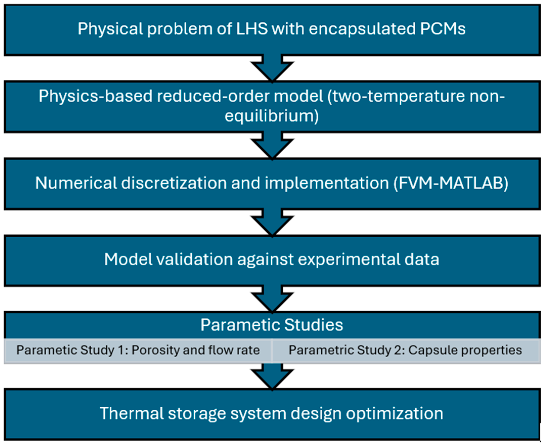
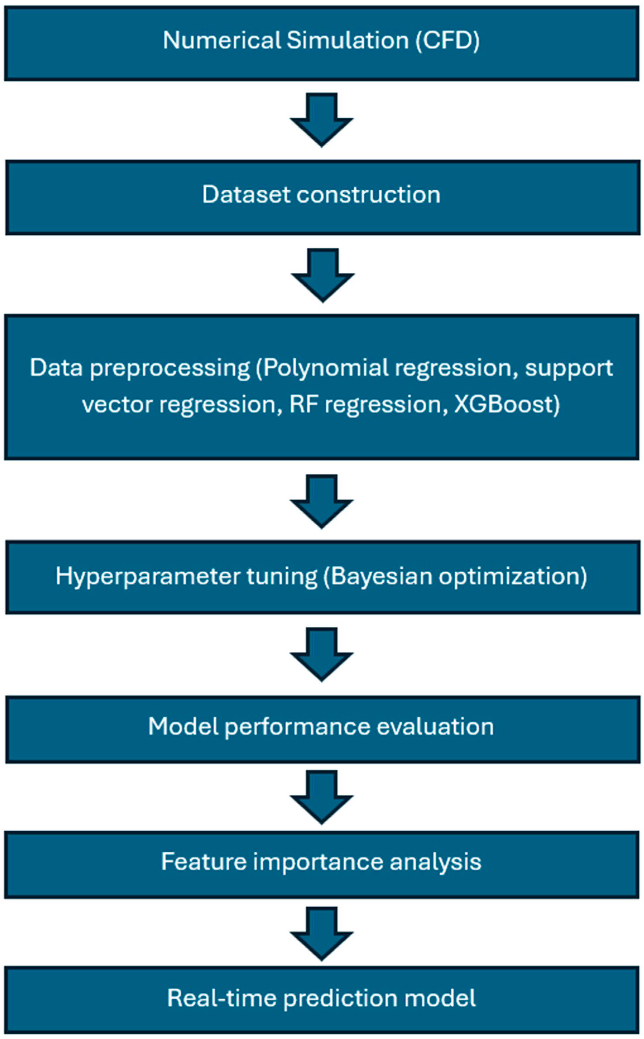
The ROM employs finite volume discretization along the axial direction, dividing the storage length into discrete control volumes. Each control volume contains both HTF and PCM, with their energy equations solved simultaneously. The model uses only five grid points in the axial direction, representing a drastic reduction from the thousands of cells required in a three-dimensional CFD simulation. This coarse discretization is enabled by the one-dimensional assumption and the use of lumped heat transfer coefficients to represent interfacial phenomena. The numerical solution proceeds using an implicit time-stepping scheme, solving the coupled algebraic equations for HTF and PCM temperatures at each time level. The phase change is handled through an iterative update of the liquid fraction based on the local enthalpy and temperature. Pressure drop across the storage is calculated using empirical correlations for flow through packed beds, accounting for both viscous and inertial losses. The ROM was implemented in MATLAB, with computational efficiency being a primary advantage. While exact timing comparisons with full-order models are not provided in the paper, the five-point spatial discretization and implicit time integration enable rapid simulation of charging processes that would require substantially more computational effort with detailed CFD. The sequence of steps followed in developing this ROM—from physical simplifications to numerical implementation and solution strategy—is summarized in Figure 6.

5.1.4. Training/Snapshot Strategy

The ROM validation relied on experimental data from published literature rather than generating a dedicated training dataset. The validation case used a storage system with identical geometry to the experimental setup, matching the HTF inlet temperature (343 K), flow rate (2 L/min), and initial PCM temperature (305 K). The heat transfer coefficient on the outer tank wall was calibrated to 2.92 W/m²·K based on ambient conditions. No additional snapshot generation was performed; the model’s predictive capability was assessed by comparing its outlet temperature predictions with the measured values. The comparison between predicted and measured HTF outlet temperatures showed maximum deviations of 2.5 K throughout the charging process. The model successfully captured the thermal stabilization period when the PCM reaches its melting temperature, as well as the subsequent temperature rise after complete melting. The close agreement validated both the two-temperature framework and the enthalpy method implementation. Following validation, parametric studies explored the effects of porosity (varying capsule packing density), capsule diameter, shell thickness, and HTF mass flow rate on system performance. These studies revealed that stabilization time—the period during which PCM actively absorbs latent heat—increases with low porosity and low mass flow rate, while capsule shell thickness has negligible influence on heat transfer.

5.1.5. Model Order and Computational Cost

The model order is characterized by five spatial grid points along the axial direction, with two dependent variables (HTF and PCM temperatures) at each point. This results in approximately 10 primary state variables, plus additional variables for tracking liquid fraction and other quantities. This represents a reduction of several orders of magnitude compared to full three-dimensional CFD models that would require millions of degrees of freedom to resolve the interstitial flow and individual capsule heat transfer. The computational cost of the ROM is not explicitly quantified in terms of wall-clock time or speed-up factors. However, the use of five grid points and implicit time integration suggests simulation times on the order of seconds to minutes for typical charging scenarios. This enables rapid parametric studies and design optimization that would be prohibitive with high-fidelity models.

5.1.6. Accuracy and Validation

The primary accuracy metric is the maximum temperature deviation between predicted and measured HTF outlet temperatures, which remained below 2.5 K across the entire charging process. This corresponds to a relative error of approximately 0.7% based on the temperature difference between inlet HTF and initial PCM temperature. The model’s main limitations stem from its fundamental assumptions. The neglect of natural convection in liquid PCM may underpredict heat transfer rates for larger capsules or high-viscosity PCMs where convection becomes significant. The one-dimensional assumption breaks down for storage systems with large diameter-to-length ratios or non-uniform flow distribution. The model also requires empirical heat transfer correlations that may not be accurate outside their calibration range, and it cannot predict detailed flow patterns or local hot spots that might be important for certain applications.

5.1.7. Application and Limitations

The intended application is solar thermal storage systems where packed-bed LHS units store excess thermal energy during periods of high solar irradiation for later use. The ROM enables rapid assessment of how design parameters (porosity, capsule size) and operating conditions (flow rate, inlet temperature) affect storage capacity, charging time, and thermal efficiency. This supports optimization of storage system design for specific solar thermal installations. The model is particularly suited for system-level simulations where the LHS unit is coupled with solar collectors, heat exchangers, and thermal loads. The computational efficiency allows the storage model to be embedded in larger energy system models without becoming a bottleneck. Potential extensions could include discharging process simulation and integration with controls for optimal charge/discharge scheduling.

Notably, the model neglects convection within the liquid PCM contained in each capsule, treating heat transfer within the capsule as purely diffusive. This simplification, while computationally attractive, bypasses the need to solve the Navier–Stokes equations in the liquid region—a substantially more complex task that would increase model order by several orders of magnitude. The assumption is justified for the small capsule diameter (55 mm) and paraffin PCM with moderate viscosity, where the Rayleigh number remains below the critical threshold for significant natural convection development. However, for larger capsules or lower-viscosity PCMs, this simplification would become invalid.

5.2. Approximation-Assisted ROMs for PCM Heat Exchangers

5.2.1. System Configuration and Physical Scope

Two complementary reduced-order modeling approaches (i.e., black-box and grey-box model) for PCM-embedded heat exchangers were developed and used in thermal energy storage applications [1]. The physical system consists of n-tetradecane PCM embedded in a thermally conductive graphite matrix, forming a composite that enhances the effective thermal conductivity while maintaining high latent heat capacity. The PCM–graphite composite is integrated into a heat exchanger geometry where heat transfer fluid flows through channels, exchanging thermal energy with the PCM. The ROM development targets rapid prediction of PCM HX performance across a wide design and operating space. The design variables include PCM transition temperature, fluid mass flow rate, and PCM slab thickness, defining a three-dimensional parameter space that must be explored during optimization. The inlet fluid conditions (temperature and mass flow rate) vary dynamically during charging and discharging, requiring the ROM to accurately predict transient thermal behavior under time-varying boundary conditions.

5.2.2. Governing Physics Incorporated into the ROM

Two distinct ROM formulations were developed: a pure black-box model and a physics-informed grey-box model. The black-box model treats the PCM HX as an input–output system without explicit representation of internal physics, relying entirely on data-driven correlations. In contrast, the grey-box model incorporates simplified heat transfer physics through the effectiveness–NTU (ε-NTU) method, which provides an analytical framework for heat exchanger performance. The ε-NTU method in the grey-box model represents the PCM using a two-node thermal network: one node for solid PCM at the transition temperature and one for sensible heat storage in liquid or solid regions. The effectiveness parameter characterizes the heat exchanger’s ability to transfer heat between the fluid and PCM, while the Number of Transfer Units quantifies the ratio of thermal capacitance to heat transfer resistance. This formulation captures the essential physics of heat exchange and phase transition while maintaining computational simplicity. Neither model explicitly resolves spatial temperature distributions within the PCM or detailed flow patterns in the fluid channels. Heat transfer is instead characterized through lumped parameters (effectiveness, NTU) or direct metamodel predictions (black-box). This level of abstraction enables rapid evaluation but sacrifices detailed local information about phase front progression or temperature gradients.

Unlike physics-derived reduced-order models, this approach follows a CFD-informed ROM development strategy in which high-fidelity simulations serve as a data generator for constructing a fast predictive surrogate. The overall process does not reduce the governing equations directly but instead transforms CFD outputs into an efficient reduced representation through data extraction, training, and validation stages.

5.2.3. ROM Methodology

The black-box model employs Kriging metamodeling, a Gaussian process regression technique that interpolates function values based on spatial correlation structures. Training data consisting of input parameters (fluid inlet temperature difference from PCM transition temperature, mass flow rate, PCM thickness) and output responses (PCM HX heat rate as a function of time) are generated using a validated finite-volume model. The Kriging metamodel learns the complex nonlinear mapping from inputs to transient heat rate trajectories, enabling rapid prediction for new parameter combinations not explicitly simulated during training. The grey-box model structure divides the transient thermal response into distinct periods based on the dominant heat transfer mechanism. During the primary phase change period, the ε-NTU method predicts heat transfer with the PCM maintained at its transition temperature. After phase change completion, a second period models sensible heating or cooling of fully solid or liquid PCM. Time periods demarcating these transitions are predicted using metamodel correlations trained on finite-volume simulation results. Both models operate without spatial discretization of the PCM domain, instead predicting global quantities like total heat transfer rate and outlet fluid temperature. This lumped-parameter approach enables time steps of 1 s compared to the millisecond-scale steps required for explicit finite-volume schemes, contributing significantly to computational acceleration. The overall workflow by which finite-volume simulation data are transformed into black-box and grey-box reduced-order representations is illustrated in Figure 7.

5.2.4. Training/Snapshot Strategy

The training dataset was generated using a validated two-dimensional finite-volume model that resolves conduction in the PCM–graphite composite and convection in the fluid channels. The sampling strategy employed Latin Hypercube Sampling to efficiently cover the three-dimensional design space with 38 sample points per design space (melting and solidification considered separately). This structured sampling ensures good space-filling properties and captures the design space more efficiently than random sampling. Eight corner points were added to the LHS samples to ensure the design space boundaries are adequately represented. The total training library thus consisted of 76 high-fidelity simulations (38 samples × 2 design spaces), with each simulation requiring 13 to 127 s depending on the melting/solidification time. For the black-box model, the training data consists of time series of heat rate for each sample point, while the grey-box model extracts characteristic time periods and effectiveness values from the same simulations. The finite-volume training simulations used an explicit time-stepping scheme with fine spatial resolution to ensure accuracy. The computational investment in training data generation is substantial (approximately 1–2 h total), but this one-time cost enables unlimited rapid predictions across the entire design space.

5.2.5. Model Order and Computational Cost

The model order differs fundamentally between the two approaches. The black-box Kriging metamodel has no explicit state variables, instead directly predicting output quantities from input parameters through learned correlation functions. The effective dimensionality is determined by the number of training samples that define the Gaussian process. The grey-box model has approximately 2–3 state variables representing PCM node temperatures and phase state, making it slightly more complex but still drastically simplified compared to the baseline finite-volume model with thousands of degrees of freedom. Computational performance comparisons against the finite-volume baseline revealed dramatic speed-up. The finite-volume model required an average of 44 s per verification case, while the grey-box model completed the same simulation in 2.5 s and the black-box model in 0.2 s. This yields speed-up factors of approximately 18× for the grey-box model and 220× for the black-box model on a component level. When integrated into a complete vapor compression system for thermal energy storage, the system simulation time decreased from an average of 1465 s using the finite-volume PCM HX model to 59 s using the reduced-order models. This represents a speed-up of 25–57× at the system level, enabling design optimization and control studies that would be computationally prohibitive with high-fidelity models.

5.2.6. Accuracy and Validation

Model accuracy was assessed using 1000 verification points (500 for melting, 500 for solidification) randomly sampled from the design space. The black-box model achieved a mean absolute error in fluid outlet temperature of 0.05 K, while the grey-box model had a slightly higher error of 0.10 K. Maximum errors reached 0.31 K and 0.50 K for the black-box and grey-box models, respectively, during melting processes. The grey-box model showed larger temperature deviations toward the end of the phase change process due to its simplified two-node PCM representation. The assumption of instantaneous transition between phase change and sensible heat periods introduces discontinuities not present in the actual physical system, leading to localized prediction errors. The black-box model, unconstrained by this structural simplification, achieved better accuracy through its more flexible functional form. At the system level, when integrated with a vapor compression system, the mean absolute deviation in compressor energy consumption was 0.2% for the black-box model and 0.3% for the grey-box model. Total charging time predictions showed deviations of 1.1% and 2.6%, respectively. These remarkably low system-level errors demonstrate that local temperature prediction errors do not necessarily propagate to integral performance metrics due to compensating effects.

5.2.7. Application and Limitations

The primary application is accelerated design and optimization of PCM-based thermal energy storage devices for building HVAC systems and renewable energy integration. The ROMs enable rapid evaluation of hundreds or thousands of design alternatives to identify optimal PCM selection, heat exchanger geometry, and operating strategies. The computational efficiency particularly benefits multi-objective optimization problems where Pareto frontiers must be mapped across competing objectives like capital cost, storage capacity, and round-trip efficiency. The models are also suited for system-level simulation where the PCM HX couples with vapor compression cycles, solar collectors, or building thermal loads. The near-instantaneous evaluation enables day-long or season-long simulations with hourly or sub-hourly time resolution, supporting analysis of energy cost savings, peak demand reduction, and grid interaction strategies.

Several limitations constrain the applicability of these ROMs. Both models assume one-dimensional heat transfer perpendicular to the flow direction, neglecting multi-dimensional effects that may be important for complex geometries. Natural convection within liquid PCM is not explicitly modeled, though its effects may be implicitly captured in the training data. The models do not account for PCM degradation, subcooling, or hysteresis effects that can occur in real systems after many thermal cycles. The black-box model requires substantial training data covering the entire operating range of interest, and extrapolation beyond the training domain can produce unreliable predictions. The grey-box model’s two-node PCM representation limits accuracy during transition periods between phase change and sensible heat modes. Neither approach provides detailed information about local temperature distributions or phase front locations, which may be important for identifying hot spots or optimizing internal heat transfer enhancement features.

5.3. POD-Based ROM for Direct Steam Generation Solar Thermal Power

5.3.1. System Configuration and Physical Scope

Researchers developed a Proper Orthogonal Decomposition (POD) reduced-order model specifically targeting latent heat storage processes in direct steam generation solar thermal power (DSG-STP) systems [8]. The physical configuration consists of a shell-and-tube heat exchanger where saturated steam at 10.7 bar flows through tubes while PCM undergoes phase change on the shell side. This high-temperature application (steam temperatures near 180 °C) presents unique challenges compared to lower-temperature building applications, including both vapor–liquid phase change in the HTF and solid–liquid phase change in the PCM. The ROM addresses unsteady-state heat transfer with simultaneous phase change occurring in both the PCM and the steam/water HTF. The system geometry includes internal tube arrays surrounded by PCM, with specific attention to modeling the vapor–liquid interface movement in the HTF tubes and the solid–liquid interface in the PCM region. The model scope encompasses variations in steam inlet conditions and time-dependent boundary conditions representative of solar thermal plant operation where steam generation rates fluctuate with solar irradiance.

5.3.2. Governing Physics Incorporated into the ROM

The full-order model underlying the POD-ROM combines the Lee model for vapor–liquid phase change with the enthalpy–porosity approach for PCM melting. The Lee model governs condensation and evaporation of the steam/water HTF by introducing source terms in the mass and energy equations based on the local temperature relative to the saturation temperature. The vapor mass fraction serves as the primary indicator of the phase state in the HTF domain. For PCM phase change, the enthalpy–porosity method treats the mushy zone as a porous medium with porosity equal to the liquid fraction. As the PCM melts, the liquid fraction evolves from zero (fully solid) to one (fully liquid), with momentum equations including a Darcy-type source term that suppresses velocity in the solid regions. This formulation naturally handles the moving solid–liquid interface without explicit tracking. The coupling between HTF and PCM occurs through conjugate heat transfer boundary conditions at the tube walls. The full-order model solves the complete set of conservation equations (mass, momentum, energy) in both domains using finite volume methods. Natural convection in liquid PCM is captured through the Boussinesq approximation, accounting for density-driven flow that can significantly enhance heat transfer compared to pure conduction.

5.3.3. ROM Methodology

The POD approach extracts dominant spatial patterns (modes) from an ensemble of full-order solution snapshots through singular value decomposition (SVD). Snapshots representing the temperature field at different time instants are arranged as columns in a matrix, and SVD identifies the orthogonal basis functions that optimally represent the ensemble in a least-squares sense. The energy contribution of each mode quantifies how much of the total variance it captures, allowing selection of the minimum number of modes needed to achieve a target accuracy. For the DSG-STP application, the temperature field is decomposed as a linear combination of POD basis functions with time-varying coefficients. The key reduction comes from retaining only the most energetic modes (typically 1–5) while discarding higher-order modes that contribute little to the overall variance. This compression from potentially millions of spatial degrees of freedom to a handful of coefficients enables dramatic computational savings. The POD coefficients (time-varying amplitudes of each mode) are obtained through interpolation methods rather than solving reduced-order differential equations. Snapshots at a limited number of time instants and operating conditions are generated using the full-order model, POD modes are extracted, and the coefficients for new conditions are interpolated from the snapshot database. This non-intrusive approach avoids the complexity of Galerkin projection and makes the ROM easy to implement. The sequence of steps followed in constructing this POD-based ROM is summarized in Figure 8.

5.3.4. Training/Snapshot Strategy

Training data consisted of 13 optimal trajectories generated by solving the full-order model with the Lee model and enthalpy–porosity approach. Each trajectory was sampled at 10 uniformly distributed time steps over a 0.5 s simulation window (with 0.05 s intervals), yielding 130 total snapshots. The operating parameters varied included the angle of attack (sampled in the range of −1.0 to 1.0 radians) and time, creating a two-dimensional parameter space. The full-order simulations required substantial computational effort, with each trajectory taking approximately 20 min on a single CPU core. This investment in generating high-quality training data is essential for POD-ROM accuracy, as the basis functions must adequately span the solution manifold across the operating range of interest. After extracting POD modes from the training snapshots, the modes are used to compress and reconstruct test data not included in the training set. The reconstruction error—the difference between the full-order snapshot and its POD approximation—provides a measure of how well the modes capture the essential dynamics. Acceptable reconstruction errors indicate that the POD basis is sufficiently rich.

5.3.5. Model Order and Computational Cost

The model order is characterized by the number of POD modes retained, which varied from 1 to 5 depending on the field variable and desired accuracy. For temperature predictions, using 5 POD modes achieved accumulative energy contributions exceeding 99%, meaning the retained modes capture 99% of the variance in the training data. Velocity and vapor mass fraction fields required similar mode counts. The computational speed-up achieved by the POD-ROM is substantial. For one test case (Case A), the finite volume method required approximately 4 h of simulation time, while the POD model completed the same simulation in 45.865 s. This represents a speed-up factor of approximately 314×, reducing a prohibitively expensive simulation to near-interactive speeds. The speed-up stems from multiple sources: elimination of spatial discretization (replaced by mode amplitudes), larger allowable time steps in the coefficient interpolation, and avoidance of iterative solution of nonlinear equations at each time step. The POD prediction simply evaluates a linear combination of pre-computed basis functions, requiring minimal computational effort.

5.3.6. Accuracy and Validation

Accuracy was quantified using relative mean error (RME) comparing POD predictions to full-order finite volume results. For temperature fields, the RME remained below 0.1% across all test cases, demonstrating excellent agreement. This remarkably low error reflects both the effectiveness of POD for smooth thermal fields and the adequate sampling of the parameter space during training. For vapor mass fraction—a more challenging quantity due to its discontinuous nature across phase boundaries—the POD-ROM also showed good performance when using 5 basis functions. The accumulative energy contribution reached 99.97% with 5 modes, confirming that this mode count adequately captures the vapor–liquid interface dynamics. Liquid fraction in the PCM region exhibited similar accuracy, with 5 modes yielding 99.08% energy contribution. The POD-ROM demonstrated consistent accuracy across both Case A and Case B test scenarios, which explored different inlet conditions and time ranges. The relative mean error for temperature predictions remained below 0.1% in both cases, and melting time predictions showed errors within 4.7%. The consistency across test cases indicates good generalization capability of the POD basis.

5.3.7. Application and Limitations

The intended application is fast simulation and control of thermal energy storage in DSG solar thermal power plants. In these systems, solar collectors generate steam that must be stored during periods of excess generation and retrieved during shortfalls. The POD-ROM enables rapid evaluation of storage performance under fluctuating solar input, supporting optimization of storage sizing, operating strategies, and dispatch scheduling. The computational efficiency is particularly valuable for model-based predictive control, where control decisions must be updated based on forecasted solar availability and electricity demand. The POD-ROM can be embedded in optimization algorithms that run in real-time or near-real-time, enabling closed-loop control that maximizes energy delivery or revenue while respecting system constraints.

The POD-ROM’s primary limitation is its reliance on pre-computed snapshots covering the operating range of interest. Extrapolation beyond the parameter space sampled during training can produce inaccurate results, as the POD basis may not adequately represent physics outside the training domain. The model also inherits any inaccuracies in the underlying full-order model, including limitations of the Lee model and enthalpy–porosity approach. The interpolation-based approach for obtaining POD coefficients may introduce errors at intermediate operating conditions not well-represented in the snapshot database. More sophisticated interpolation methods or larger snapshot libraries could improve accuracy but at the cost of increased training effort. The model also provides only temperature, velocity, and phase fraction fields—derived quantities like local heat fluxes or stress distributions require post-processing. A practical limitation noted by the authors is the relatively small number of training samples (13 trajectories) used in this demonstration. While sufficient for the two-parameter space explored, more complex systems with additional degrees of freedom would require substantially more snapshots to adequately sample the solution manifold. The linear nature of POD may also limit accuracy for highly nonlinear phenomena like turbulent convection or complex phase change behavior.

5.4. Analytical 1D ROM for Metal–Polymer Composite Heat Exchangers

5.4.1. System Configuration and Physical Scope

A ROM was proposed for a novel LHS system utilizing additively manufactured metal–polymer composite heat exchangers [2]. The physical configuration consists of metal fin-wires arranged in a tube-bank geometry, with the interstitial spaces filled by polymer encapsulating the PCM. This cross-media approach leverages additive manufacturing to create integrated structures where conductive metal fins enhance heat transfer while the polymer provides in-built macro-encapsulation for the PCM. The system geometry is reduced to a segment-level model comprising a single PCM–wire cylindrical domain based on the tube-bank arrangement. Each cylindrical domain represents the PCM wrapped around one metal wire, with the radius determined by the wire spacing (transverse pitch ST and longitudinal pitch SL). This geometric abstraction enables analysis of the fundamental heat transfer unit cell rather than the entire heat exchanger, dramatically reducing model complexity.

5.4.2. Governing Physics Incorporated into the ROM

The ROM assumes one-dimensional radial conduction inside the PCM cylinders enveloping the metal wires, neglecting both axial conduction along the wire direction and convection in the liquid PCM. This simplification is justified for low-Stefan-number applications where conduction dominates and for geometries with high aspect ratios where radial resistance significantly exceeds axial resistance. The metal wire is treated as having infinite thermal conductivity in the axial direction but finite radial conductivity that couples to the PCM through the wire–PCM interface. Heat transfer from the heat transfer fluid to the PCM occurs through convective boundary conditions on the wire surface. The convective heat transfer coefficient is obtained from standard correlations for flow over heated cylinders in tube banks. The PCM phase change is modeled using thermal resistance and energy conservation principles, with latent energy analytically computed for the cylindrical domain and then time-integrated for the entire TES assembly. Notably, the model neglects sensible thermal capacity, making it applicable primarily for low-Stefan-number applications where latent heat dominates over sensible heat. The model also assumes negligible overlaps between adjacent PCM cylinders, though geometric studies were conducted to assess the impact of overlapping regions where this assumption breaks down.

5.4.3. ROM Methodology

The analytical ROM is constructed using thermal resistance and energy conservation principles rather than discretized differential equations. The heat flow from the HTF through the convective boundary layer, across the wire, and into the PCM is modeled as a series of thermal resistances. The melting process advances radially inward from the heated wire surface, with the position of the solid–liquid interface tracked as a function of time. Energy conservation applied to the moving phase boundary yields an ordinary differential equation for the interface position. This equation is solved analytically or semi-analytically, providing explicit expressions for the temperature distribution and interface location as functions of time. The total latent energy stored is obtained by integrating the energy released during solidification (or absorbed during melting) over the volume of PCM that has undergone phase change. The segment-level model is then extended to the entire TES by multiplying the energy stored in a single cylindrical domain by the total number of wire–PCM units. This scaling approach assumes all units behave identically, which is valid for uniform inlet conditions and negligible flow maldistribution. The computational cost is minimal since the ROM involves evaluating analytical or semi-analytical expressions rather than solving large systems of equations. The general workflow that transforms the original multidimensional heat transfer problem into an efficient one-dimensional reduced-order formulation is presented in Figure 9.

5.4.4. Training/Snapshot Strategy

Rather than training on high-fidelity simulation snapshots, the 1D ROM was validated against a 2D axisymmetric CFD model. The CFD model represents a single cylindrical PCM domain with radial and axial heat conduction, providing a reference solution against which the 1D assumption can be assessed. A 2D Cartesian CFD model was also developed to study the geometric behavior of overlaps between adjacent cylinders and their effect on model accuracy. The validation studies varied three non-dimensional parameters across wide ranges: (i) τ (dimensionless time, ranging from 0.03 to 300), (ii) BiLR (Biot number based on axial conductance, 0.03 to 300), and (iii) R_wire (resistance ratio, 0.01 to 100). These parameters characterize the relative importance of different heat transfer mechanisms and resistance components, allowing assessment of where the 1D approximation is valid. Optimum geometric ranges of wire spacings and sizes were identified through these parametric studies. Spacing ratios of ST/SL = 1.27 and 3.5 at higher r_max were found to yield accurate results. For most parameter combinations, the 1D ROM correlated well with the 2D axisymmetric reference model to within 10%, except at extreme ranges where BiLR ≥ 300 or R_wire ≥ 10 led to significant axial conduction deviating from the 1D assumption.

5.4.5. Model Order and Computational Cost

The model order is characterized by a single spatial coordinate (radial position) with analytical or semi-analytical solutions obviating the need for discretization. The primary unknowns are the interface position as a function of time and the temperature distribution in the solid and liquid regions, which can be expressed in closed form or require solution of a single ordinary differential equation. Computational cost is not explicitly quantified in terms of speed-up factors or wall-clock times. However, the analytical nature of the model suggests near-instantaneous evaluation suitable for real-time applications or extensive design optimization studies. The model is particularly appropriate for design optimization problems where the ROM must be evaluated thousands or millions of times to identify optimal configurations.

5.4.6. Accuracy and Validation

The primary accuracy metric is the comparison of performance parameters (such as time to reach 90% melting) between the 1D ROM and the 2D CFD reference. For the ranges where the 1D assumption is valid, deviations remain within 10%. This accuracy is achieved without any tuning or calibration—the ROM is purely based on first principles with no adjustable parameters beyond standard material properties and heat transfer correlations. The geometric studies using 2D Cartesian CFD revealed that overlapped areas between adjacent cylindrical domains can introduce errors when their extent becomes significant. The model accuracy depends on selecting appropriate spacing ratios that minimize these overlaps while maintaining reasonable packing density. Optimal spacing ratios identified through these studies help guide practical system design. For extreme parameter combinations outside the validity range (BiLR ≥ 300, indicating dominant axial conduction in the wire), deviations can reach 86%. However, for typical applications with BiLR < 3 where fluid-side resistance dominates, the model unconditionally correlates well with 2D CFD regardless of R_wire value. This delineation of the validity domain helps users understand when the 1D ROM can be trusted.

5.4.7. Application and Limitations

The target application is peak-load shifting for building cooling through thermal energy storage. The lightweight, low-cost metal–polymer composite HX enables integration of latent heat storage in building HVAC systems, charging the PCM during off-peak hours when electricity is inexpensive and discharging during peak demand periods. The 1D ROM supports rapid design of these systems, determining optimal PCM selection, wire dimensions, and spacing. The model is also applicable to pulsed-power cooling applications where transient high heat loads must be managed. In such applications, the ROM enables assessment of how quickly the PCM can absorb heat pulses and how long before thermal management fails. The analytical nature makes the model suitable for parametric design studies exploring trade-offs between weight, volume, cost, and thermal performance.

The neglect of sensible thermal capacity limits applicability to low-Stefan-number situations where latent heat dominates. For PCMs with low latent heat or applications with large temperature excursions, the sensible heat contributions cannot be ignored. The assumption of 1D radial conduction breaks down when axial conduction becomes significant (large BiLR or R_wire), requiring users to verify they are operating within the valid parameter ranges. Natural convection in liquid PCM is neglected, which may underpredict heat transfer for materials with low viscosity and moderate-to-large wire diameters [6]. The model also assumes perfect thermal contact between the wire and PCM, whereas in reality, interfacial thermal resistance may exist. Geometric overlaps between adjacent cylindrical domains are not rigorously accounted for, though their impact has been studied and optimal spacing ratios identified to minimize errors.

5.5. CFD Results-Based Look-Up Table ROMs

5.5.1. System Configuration and Physical Scope

A novel approach was introduced to generate reduced-order models for LHS systems with macro-encapsulated PCM, utilizing CFD simulation results as the basis [9]. The physical system consists of spherical capsules filled with PCM arranged in layers within a storage tank. Hot HTF flows upward through the tank, charging the PCM by melting it through convective heat transfer at the capsule surfaces and conductive/convective heat transfer within each capsule. The ROM approach focuses on a single capsule as the fundamental modeling unit, recognizing that system behavior emerges from the collective response of many such capsules. This segment-level reduction is analogous to the approach taken by Kailkhura et al. [2], but here, the detailed capsule dynamics are captured through comprehensive CFD simulations rather than analytical approximations. Three levels of modeling fidelity were explored: (1) PCM only (CFD-PCM), (2) PCM with an air gap and capsule wall (CFD-PCM-air-wall), and (3) the full system including surrounding HTF (CFD-PCM-air-wall-HTF).

5.5.2. Governing Physics Incorporated into the ROM

The CFD models capture detailed heat transfer physics within and around individual PCM capsules. The PCM phase change is modeled using the enthalpy–porosity method, which naturally handles the moving solid–liquid interface and allows for mushy zone formation. Close-contact melting (CCM) at the bottom of the capsule—where the liquid PCM layer becomes very thin as solid PCM sinks due to gravity—is resolved by the CFD mesh. Natural convection within liquid PCM is fully captured through solution of the Navier–Stokes equations coupled with energy conservation. The Boussinesq approximation relates density variations to temperature differences, driving buoyancy-induced flow. This convection significantly affects melting rates, particularly in the later stages of charging when large liquid regions have formed. For the models including the capsule wall, conjugate heat transfer across the shell is resolved, accounting for thermal resistance and capacitance of the wall material. The CFD-PCM-air-wall-HTF variant further includes the HTF flow field around the capsule, capturing the development of thermal boundary layers and wake effects that influence heat transfer coefficients. Each level of fidelity adds computational cost but potentially improves prediction accuracy.

5.5.3. ROM Methodology

The ROM methodology consists of two stages: (1) offline CFD simulation campaign to populate look-up tables, and (2) online rapid evaluation using the tables within a system simulation model. In the offline stage, detailed CFD simulations of a single capsule are performed for systematically varied boundary conditions. The results are written into look-up tables that contain the charging power of one capsule as a function of the enthalpy stored and the boundary conditions (HTF temperature, heat transfer coefficient or mass flow rate). The look-up tables effectively compress the CFD results into a functional relationship $Q = f\left(H, T_{HTF}, k or \dot{m}\right)$, where $Q$ is the instantaneous heat transfer rate, $H$ is the total enthalpy stored in the capsule, and the remaining arguments characterize the thermal driving force and convection strength. This representation captures the essential nonlinear relationship between driving conditions and heat transfer without requiring solution to the full CFD problem. In the online stage, the system simulation model discretizes the storage tank into layers, with each layer containing multiple capsules. At each time step, the enthalpy of capsules in each layer is known, allowing the look-up table to be queried to determine the heat transfer rate. This rate is used to update the enthalpy and HTF temperature, marching forward in time. The approach assumes capsules within a layer behave identically and neglects inter-layer heat transfer, which are reasonable approximations for most storage configurations. The development workflow is illustrated in Figure 10.

5.5.4. Training/Snapshot Strategy

The offline CFD simulations were performed for 6–18 different combinations of boundary conditions depending on the model variant. The parameters varied included HTF temperature (22.5–35 °C), heat transfer coefficient (114–285 W/m²·K for fixed coefficient models), and mass flow rate (5.893–7.237 kg/min for the HTF-included model). Each CFD simulation tracked one capsule from the fully solid state through complete melting, providing time series of heat transfer rate and stored enthalpy. Each individual CFD simulation lasted up to more than two weeks on one CPU core of a workstation. This substantial computational investment is incurred once during the offline training phase, but the resulting look-up tables enable thousands of rapid online evaluations. The approach is viable when access to computing clusters allows many simulations to run in parallel, amortizing the wall-clock time for training data generation. The CFD mesh for the PCM domain contained 60,000 cells with strong refinement near the bottom boundary to resolve close-contact melting. Mesh independence studies confirmed this resolution adequately captures the essential physics without excessive computational cost. The CFD models were implemented in OpenFOAM and validated against experimental measurements before use in training data generation.

5.5.5. Model Order and Computational Cost

The look-up table (LUT) ROM has no explicit state variables in the traditional sense—it operates by table interpolation rather than solving differential equations. The effective model complexity is determined by the resolution of the look-up table grid, which spans 2–3 dimensions depending on whether a constant heat transfer coefficient or varying mass flow rate is considered. The tables are queried using efficient interpolation functions, with computational cost dominated by table read operations. The computational speed-up achieved is extraordinary. The fastest ROM variant completed system simulations in approximately 5 s, while the reference CFD simulation of the full storage would take up to two weeks. This represents a speed-up factor of approximately 80,000×, among the highest reported for any LHS ROM. Even accounting for time spent reading from look-up tables—which can be further optimized by compiling to C code—the speed-up factor remained above 50,000×.

5.5.6. Accuracy and Validation

The ROM was validated against experimental measurements from a two-layer storage system. The temporal mean deviation of energy content between experiments and the ROM was only 5%, demonstrating excellent agreement despite the multiple simplifications inherent in the segment-level approach. This validation included realistic effects like heat losses and non-uniform HTF distribution that are challenging to capture in simplified models. Comparisons between the three model variants revealed that including the capsule wall is essential for accurate predictions, especially when wall thermal conductivity is significantly higher than PCM conductivity. The HTF flow field, however, can be replaced by a properly defined convective boundary condition without substantial loss of accuracy, simplifying the CFD training simulations. These findings provide guidance on the minimum level of physics fidelity required.

5.5.7. Application and Limitations

The intended application is rapid design and optimization of large-scale LHS systems with macro-encapsulated PCM. The ROM enables evaluation of different capsule sizes, materials, and tank geometries across varying operating conditions. The speed-up makes it feasible to simulate full charge–discharge cycles over days or weeks, supporting techno-economic analysis and control strategy development.

The primary limitation is the substantial upfront computational cost for CFD training data generation, requiring access to computing clusters for parallel execution. The approach is most valuable when many design iterations or long-duration simulations justify this investment. The look-up tables are specific to the capsule geometry and materials studied—new configurations require new CFD campaigns. Additionally, the model assumes uniform behavior within each tank layer and neglects potential flow maldistribution or hot spots that could occur in large storage systems.

5.6. Machine Learning-Based Reduction: Artificial Neural Networks for Finned Enclosures

5.6.1. System Configuration and Physical Scope

Just recently, the PCM melting dynamics in a rectangular enclosure with dimensions of 50 × 50 mm was predicted using artificial neural networks (ANNs) [125]. The configuration includes a 5 mm thick aluminum heater plate maintained at constant temperature (70 °C) on the left side. Inside the enclosure are two fins with varying lengths of 12.5 mm, 25 mm, and 37.5 mm, allowing investigation of fin geometry effects on melting behavior. The physical scope encompasses the solid–liquid phase change process and the evolution of the melting front over time.

5.6.2. Governing Physics Incorporated into the ROM

The numerical model accounts for the phase change process of PCM through energy conservation and momentum equations. The enthalpy–porosity method is employed to treat the mushy zone as a porous medium during melting, equating the liquid-phase volume fraction to the porosity. The model captures heat conduction in both solid and liquid phases, natural convection effects during melting, and the temporal evolution of the solid–liquid interface. These governing equations provide the basis for generating training data through numerical simulation.

5.6.3. ROM Methodology

The ROM methodology employs ANNs trained in numerical simulation data. Spatial coordinate data of the solid–liquid interface at various time steps extracted from numerical contours are used to train the ANN model. The ANN learns the dynamic melting behaviors of PCM under varying conditions, subsequently enabling prediction of melting front evolution and temperature distribution. This represents a data-driven surrogate modeling approach that replaces expensive numerical simulations. The data-driven workflow is summarized in Figure 11.

5.6.4. Training/Snapshot Strategy

The training approach uses coordinate data extracted from numerical simulation results at three different fin lengths (12.5 mm, 25 mm, and 37.5 mm). After training on these three geometries, the ANN model is employed to predict melting behavior at intermediate fin lengths of 20 mm and 30 mm, which were not included in the training dataset. This strategy tests the ANN’s ability to interpolate across the geometric parameter space and predict results for conditions not explicitly simulated during training.

5.6.5. Model Order and Computational Cost

The computational speed-up achieved by the ANN approach is dramatic. Simulating PCM melting for two intermediate fin length cases (20 mm and 30 mm) via traditional numerical methods requires approximately 6 days of computational time. In contrast, the trained ANN model completes predictions in just a few minutes, representing a computational acceleration of roughly 1440× while maintaining high accuracy. This substantial reduction enables rapid thermal system design exploration and optimization.

5.6.6. Accuracy and Validation

The ANN model demonstrates exceptional accuracy with low error metrics. For PCM melting front training, mean absolute error (MAE), mean squared error (MSE), and Pearson’s correlation coefficient (R) values are approximately 0.014, 0.03, and 0.99, respectively. For temperature distribution, corresponding metrics are around 0.016, 0.03, and 0.99. Validation on unseen fin lengths (20 mm and 30 mm) yields MAE, MSE, and R values of approximately 0.02, 0.03, and 0.98, demonstrating robust generalization. Graphical comparisons show predicted melting fronts and temperature distributions closely aligned with numerical simulation results across all time intervals. The ANN approach is intended to advance thermal management system designs through efficient prediction of PCM melting behavior. By reducing simulation time from approximately 6 days to a few minutes with high accuracy, the methodology enables practical design optimization of finned PCM enclosures.

5.6.7. Application and Limitations

The approach is adaptable to various thermal management applications where rapid performance assessment is required during iterative design processes. While the ANN model shows high accuracy for interpolation within the training parameter range, the study does not extensively explore extrapolation beyond the geometric range covered by the three training cases. The reliance on numerical simulation data for training introduces the same physical assumptions inherent in the CFD approach. Additionally, the transferability of the trained model to different enclosure sizes, fin materials, or PCM types requires validation and potentially retraining.

5.7. Machine Learning-Based Reduction: XGBoost for Triplex-Tube Systems

5.7.1. System Configuration and Physical Scope

Another study developed a machine learning prediction method for a triplex-tube thermal energy storage system incorporating PCM with Y-shaped fins to enhance heat transfer [126]. The configuration includes design variables encompassing fin angle (10–20°), fin width (5–15 mm), fin design characteristics, and operational conditions including heat transfer fluid temperature (60 °C). The physical scope encompasses the melting response time of PCM, representing the duration required for complete or substantial phase transition under specified thermal conditions.

5.7.2. Governing Physics Incorporated into the ROM

The numerical model is based on the enthalpy–porosity method for simulating the melting process. The governing equations include the continuity equation, momentum equations with Boussinesq approximation for natural convection, and energy conservation accounting for phase change latent heat. The liquid fraction of PCM is calculated as a function of temperature relative to phase change limits, and the mushy zone constant is a key element controlling the transition. The model also accounts for boundary conditions where no-slip conditions are applied at solid surfaces.

5.7.3. ROM Methodology

Four machine learning algorithms were employed to predict melting response time: polynomial regression, support vector regression (SVR), random forest (RF) regression, and extreme gradient boosting (XGBoost). Hyper-parameter optimization was performed using a Bayesian approach to refine each model’s performance. The XGBoost model demonstrated superior predictive capability compared to alternative approaches, emerging as the optimal model class for this prediction task. The general workflow for developing the ML-informed ROM model is presented in Figure 12.

5.7.4. Training/Snapshot Strategy

The training dataset comprises 60 numerical simulation cases with melting response times ranging from 15 to 45 min under varying design and operational conditions. Prior to model development, variable independence was validated to ensure robust predictions. The dataset encompasses variations in fin angle, fin width, and heat transfer fluid temperature, capturing the interaction effects between these design parameters on system response time.

5.7.5. Model Order

The model order is not explicitly quantified, but the trained XGBoost model can evaluate numerous design candidates in negligible time compared to a full numerical simulation. While a precise speed-up factor is not reported, the approach substantially accelerates design-space exploration.

5.7.6. Accuracy and Validation

The XGBoost model achieved 92% accuracy in predicting the melting response time, outperforming the other algorithms (SVR exhibited significant overfitting on the test set). Feature importance analysis revealed that fin width and HTF temperature are the dominant factors, contributing 51% and 47% to the prediction variance, respectively, while fin angle has only a marginal influence (2%).

5.7.7. Application and Limitations

The methodology enables quantitative prediction of melting response time for triplex-tube TES systems, supporting optimization of fin geometry for enhanced thermal performance. Limitations include the absence of extensive testing for extrapolation beyond the 15–45 min response-time range or for PCM properties substantially different from those used in training. Transferability to other triplex-tube configurations or PCM materials would require validation through additional simulations.

5.8. Physical Validity Limits of Simplified ROMs

The simplified ROMs surveyed above—particularly physics-based reduced models like two-temperature non-equilibrium [81] and 1D analytical formulations [2]—operate within specific validity ranges defined by dimensionless parameters. Understanding these limits is essential for appropriate model selection and avoiding erroneous predictions outside the design space.

5.8.1. Two-Temperature Non-Equilibrium Models

The two-temperature non-equilibrium model for packed-bed systems [81], detailed in Section 5.1, operates under a set of simplifying assumptions that define its range of applicability. This approach reduces the full three-dimensional packed bed to a one-dimensional axial formulation by assuming negligible radial temperature gradients and uniform flow distribution across the bed cross-section. Heat transfer within each PCM capsule is treated as conduction-dominated, neglecting natural convection in the liquid phase, and the phase change is assumed to occur isothermally within each capsule. These assumptions are quantified through several dimensionless parameters that establish the model’s validity limits. The Biot number ($Bi=hD/k_{PCM}$) must remain below 0.1 to justify the lumped capacitance assumption within each capsule; for larger Biot numbers, intra-capsule temperature gradients become significant and the model’s accuracy degrades. The Rayleigh number ($Ra=g\beta \Delta T{D}^3/\left(\nu \alpha \right)$) should be less than ${10}^3$ to ensure that natural convection within the liquid PCM remains negligible—above this threshold, buoyancy-driven flow enhances heat transfer and the conduction-only assumption under-predicts melting rates. The Péclet number ($Pe=uD/{\alpha }_{HTF}$) characterizes the ratio of convective to diffusive heat transport in the HTF; for $Pe>10$, axial dispersion effects may become significant and the plug-flow assumption weakens. Additionally, the bed aspect ratio ($L/D$) should exceed 5 to justify the one-dimensional radial gradient assumption, and capsule diameters are typically limited to $D<100$ mm to maintain conduction dominance. When these parametric conditions are violated—for instance, in systems with large capsules, low-viscosity PCMs, or non-uniform flow distribution—the simplified model’s predictions become unreliable, and more sophisticated ROM approaches (such as those incorporating intra-capsule gradients or convection effects) must be employed.

5.8.2. 1D Analytical Thermal Resistance Models

The one-dimensional analytical thermal resistance model [2] presented in Section 5.4, developed for metal–polymer composite heat exchangers, rests on several fundamental assumptions that define its operational envelope. The model reduces the heat transfer problem to purely radial conduction, neglecting axial conduction along the wire direction and any natural convection within the liquid PCM. It further assumes negligible sensible heat storage (applicable only for low-Stefan-number conditions) and perfect thermal contact at the PCM–wall interface. These assumptions are quantified through a set of dimensionless parameters that delineate the model’s validity range. The Stefan number ($Ste=c_p\Delta T/L$) must remain below 0.1 to justify the neglect of sensible heat; for larger values, sensible heat storage becomes non-negligible, and the model under-predicts total energy storage and misrepresents interface motion. The axial Biot number ($B{i}_{LR}$)—characterizing the ratio of axial conduction to radial resistance—should be less than 3; when $B{i}_{LR}\ge 300$, axial conduction dominates and the 1D radial assumption fails catastrophically, with reported errors reaching 86% [2]. The resistance ratio ($R_{wire}$) must remain below 10 to ensure that wire thermal resistance is negligible compared to PCM resistance; for $R_{wire}\ge 10$, the wire must be modeled explicitly. The Rayleigh number ($Ra$) should be less than ${10}^3$ to maintain the conduction-dominated regime; beyond this threshold, natural convection enhances melting rates and the pure conduction model under-predicts heat transfer. Finally, the Fourier number ($Fo=\alpha t/D^2$) must exceed approximately 0.1 for the quasi-steady moving-boundary assumption to hold—at very early times (small $Fo$), transient effects not captured by the quasi-steady formulation become significant. When these parametric conditions are satisfied simultaneously, the 1D analytical model provides rapid and reliable predictions (within 10% of 2D CFD reference solutions). However, deviations outside these ranges necessitate either the use of more comprehensive ROMs that relax the underlying assumptions or direct recourse to full-order simulation.

5.8.3. Packed-Bed Models with Uniform Capsule Assumption

Many packed-bed reduced-order models, including the two-temperature non-equilibrium formulation discussed in Section 5.1, rely on the simplifying assumption that all capsules within a given layer behave identically [81]. This assumption, while computationally convenient, becomes invalid under several practical conditions. First, flow maldistribution across the bed cross-section—caused by inlet geometry, non-uniform packing, or viscous fingering—leads to variations in local HTF velocity that produce differential charging rates among capsules nominally at the same axial position. Second, manufacturing tolerances in capsule dimensions, wall thickness, or PCM filling can introduce property variations that cause otherwise identical capsules to respond differently to the same thermal boundary conditions. Third, close-contact melting phenomena, where the solid PCM sinks and establishes a thin liquid layer at the heated surface, can create capsule-to-capsule variations in heat transfer that depend on local orientation and packing arrangement. Fourth, wall effects near the container boundary produce localized variations in porosity and flow velocity that deviate from the idealized uniform packing assumed in one-dimensional models. Quantitatively, when the coefficient of variation (defined as the ratio of the standard deviation to the mean) of local HTF velocity exceeds 10–15%, layer-averaged models may significantly mispredict charging uniformity and overall system performance. In such cases, the uniform-capsule assumption must be relaxed, either by incorporating stochastic representations of capsule behavior, using multi-channel or multi-layer models that resolve radial variations, or employing CFD-derived look-up tables that capture capsule-to-capsule interactions.

5.8.4. Convection-Simplified Models (Enhanced Conductivity)

A common simplification employed in many PCM reduced-order models, particularly those targeting design-space exploration where computational speed is paramount, is the approximation of convective heat transfer through an enhanced effective thermal conductivity of the form $k_{eff}=Nu\cdot k$. This approach lumps the complex, multi-dimensional effects of buoyancy-driven flow into a single scalar multiplier, thereby avoiding the need to solve the coupled momentum equations. However, the validity of this simplification is contingent upon several stringent conditions. First, the convection must be steady and well-developed—the model cannot capture the transient onset of convection or flow regime transitions during the melting process. Second, the flow pattern must be approximately known and consistent with the assumed correlation structure (e.g., a single dominant recirculation cell in a cylindrical enclosure). Third, the Nusselt number correlation employed must be specifically calibrated for the geometry and Rayleigh number range of interest; using correlations developed for different configurations or extrapolating beyond their validated range introduces significant uncertainty. The typical validity range for common Nusselt correlations lies between ${10}^3<Ra<{10}^6$; within this window, the enhanced conductivity approximation can reasonably capture the time-averaged heat transfer enhancement. Below $Ra\approx {10}^3$, conduction dominates and the enhancement is unnecessary; above $Ra\approx {10}^6$, the flow may transition to unsteady or turbulent regimes that the steady correlation cannot represent. Outside this range, extrapolation of the Nusselt number becomes unreliable, and the enhanced conductivity model may either under-predict or over-predict heat transfer rates by substantial margins. Practitioners must therefore verify that their operating conditions fall within the correlation’s validated range and remain alert to situations where the convection pattern deviates from the assumed form—such as in geometries with multiple recirculation cells, strong three-dimensional effects, or during the early stages of melting when convection is first establishing itself.

5.8.5. General Guidance for Model Selection Based on Dimensionless Parameters

The preceding analysis of validity limits for various simplified ROMs can be synthesized into practical guidance for model selection based on the dominant characteristics of the system under consideration. For systems employing small capsules (diameter less than 50 mm), simplified models such as the two-temperature non-equilibrium formulation [81] are generally valid when the Biot number remains below 0.1 (ensuring negligible internal temperature gradients) and the Rayleigh number is less than ${10}^3$ (ensuring conduction-dominated heat transfer within the capsule); when these conditions are violated, models that incorporate internal gradients—such as two-temperature formulations with intra-capsule resolution or CFD-derived look-up tables—become necessary. For large capsules (diameter exceeding 100 mm), natural convection is almost invariably significant, rendering conduction-dominated simplified models invalid; in such cases, practitioners must resort to CFD-based ROMs or machine learning surrogates trained on convection-resolved simulation data. Systems utilizing low-conductivity PCMs (thermal conductivity below 0.3 W/m·K) face stringent Biot number constraints that necessitate very small capsule diameters to maintain validity; when fin enhancements are employed to overcome this limitation, the ROM must resolve the fin geometry explicitly rather than relying on homogenized effective property approximations. Applications involving high temperature differences (ΔT exceeding 50 K) must verify that the Stefan number remains below 0.1 to justify neglecting sensible heat; this typically requires very large latent heat capacities, and when this condition is not met, the ROM must either include sensible heat contributions explicitly or employ a full enthalpy-based formulation. For systems where natural convection is known to be dominant—characterized by Rayleigh numbers well above ${10}^3$—conduction-only or enhanced-conductivity models are fundamentally inadequate; instead, projection-based methods that retain velocity fields (such as POD with full Navier–Stokes snapshots) or convection-resolved look-up tables must be employed. Finally, for long-term cyclic operation extending over many charge–discharge cycles, even ROMs that perform accurately over a single cycle may exhibit drift due to accumulated energy conservation errors; validation over multiple cycles is essential to confirm that the model captures steady-periodic behavior correctly. Reporting these dimensionless parameters alongside ROM results—as advocated throughout this section—would enable users to assess the applicability of published models to their specific systems and identify when the validity limits have been exceeded, thereby guiding the selection of more sophisticated ROM approaches when necessary.

5.9. Cross-Case Comparative Analysis

To synthesize the individual case studies presented in Section 5.1, Section 5.2, Section 5.3, Section 5.4, Section 5.5 and Section 5.6,

Table 4. Comparative analysis of ROM case studies for PCM-based LHS systems.

Case Study	Core Challenges Addressed	ROM Category	LHS Configuration	Accuracy Metric	Speed-Up	Key Trade-Off Achieved
Two-temperature packed bed [81]	Geometry/boundary sensitivity; multi-timescale	Physics-based (porous medium)	Packed-bed spherical capsules	2.5 K max deviation	Not reported	Interpretability vs. spatial resolution
Kriging metamodel [1]	Latent heat nonlinearity; parameter sensitivity	Data-driven (black-box)	PCM-embedded HX	0.05 K MAE	220×	Speed vs. physical transparency
ε-NTU grey-box [1]	Latent heat nonlinearity; multi-timescale	Hybrid (physics+data)	PCM-embedded HX	0.10 K MAE	18×	Physical consistency vs. flexibility
POD interpolation [8]	Moving boundaries; conjugate heat transfer	Projection-based	Shell–tube DSG-STP	<0.1% RME	314×	Field preservation vs. data dependence
1D analytical [2]	Moving boundaries; conduction dominance	Physics-based (analytical)	Metal–polymer composite HX	10% validation	Not reported	Simplicity vs. validity range
CFD look-up table [9]	Moving boundaries; CCM; convection	Precomputed database	Macro-encapsulated spherical	5% energy error	80,000×	Offline cost vs. runtime speed
ANN [125]	Nonlinear melting; geometric variation	ML-based (neural network)	Finned rectangular enclosure	MAE 0.02, R2 0.98	~2000×	Geometric flexibility vs. extrapolation
XGBoost [126]	Parameter interaction; response time	ML-based (gradient boosting)	Triplex-tube with Y-fins	92% accuracy	Not reported	Design exploration vs. interpretability

provides a horizontal comparison across six key dimensions: (1) core physical challenges addressed (as identified in Section 4.2), (2) ROM methodological category, (3) LHS configuration, (4) reported accuracy, (5) computational speed-up, and (6) achieved trade-offs. This comparative framework reveals systematic relationships between application requirements and ROM design choices.

The comparison reveals several systematic patterns. First, physics-based ROMs (two-temperature, 1D analytical) excel at addressing moving-boundary problems and offer high interpretability, but their validity is constrained to specific parameter ranges and they provide limited speed-up. Second, projection-based methods (POD) uniquely preserve spatial field information while achieving substantial compression (314×), making them ideal for applications requiring detailed thermal field knowledge such as digital twins. Third, data-driven surrogates (Kriging, ANN, XGBoost) achieve the highest speed-ups (up to 2000×) and handle geometric complexity effectively, but their black-box nature limits physical insight and extrapolation capability. Fourth, hybrid approaches (ε-NTU grey-box, CFD look-up tables) strategically combine a physics-based structure with data-driven components, offering balanced trade-offs: the grey-box model maintains physical interpretability while achieving 18× speed-up, while the look-up table trades enormous offline computational investment for unprecedented runtime performance (80,000×).

This comparative analysis demonstrates that ROM selection must be guided by the dominant physical challenges of the target application. For systems where moving-boundary dynamics are critical, POD or CFD look-up tables are preferred. When geometric parameter variation is the primary concern, ML-based surrogates offer the most flexibility. For system-level integration where interpretability matters, physics-based or hybrid grey-box models provide the necessary transparency. The mapping between application objectives and recommended ROM approaches is further developed in Section 6.5 as a practical decision-making framework.

5.10. Summary of ROMs for PCM-Based LHS Systems

The reviewed ROMs for PCM-based latent heat storage systems span five major reduction philosophies: physics-reduced analytical models, grey-/black-box metamodels, projection-based POD models, CFD-results-based look-up tables, and purely data-driven machine learning surrogates, each reducing computational cost in fundamentally different ways while retaining varying levels of physical fidelity. Analytical and two-temperature porous-medium ROMs simplify governing equations through dimensional reduction and thermal resistance analogies, yielding very low model order and high interpretability but limited geometric flexibility and validity ranges. Grey-box ε-NTU and black-box Kriging metamodels remove spatial resolution entirely and rely on training from finite-volume data to predict global performance metrics, achieving 18×–220× speed-ups with sub-Kelvin errors and strong suitability for system-level simulations. POD-based ROMs compress full CFD spatial fields into a few dominant modes, preserving temperature and phase distributions with over 300× acceleration and <0.1% error, making them ideal for control and digital twin applications but dependent on representative snapshot databases. CFD look-up table ROMs precompute detailed capsule physics offline and replace online PDE solving with table interpolation, producing extreme speed-ups (~80,000×) at the expense of large upfront CFD cost and geometry specificity. In contrast, ANN and XGBoost surrogates learn melting dynamics and response times directly from CFD data, enabling ~1440× acceleration and high statistical accuracy for complex finned and triplex-tube geometries, though with limited extrapolation capability and reduced interpretability. Collectively, these approaches demonstrate a trade-off between interpretability, transferability, data dependence, and computational speed, indicating that ROM selection must be aligned with the intended application, whether for design optimization, system simulation, control, or geometric exploration.

Table 5. Summary of ROMs for LHS systems for the past five years.

ROM Method	LHS Configuration	Physics	Error Metrics	Error/ Accuracy	Speed-Up	Application
Two-temperature non-equilibrium [81]	Packed-bed spherical capsules	Conduction + enthalpy method	Temperature deviation: Maximum absolute difference between predicted and measured HTF outlet temperature (2.5 K corresponds to ~0.7% relative error based on 40 K driving temperature difference)	2.5 K (max)	Not reported	Solar thermal storage
Kriging metamodel (Black-box) [1]	PCM-embedded HX	Heat transfer (metamodel)	Mean absolute error (MAE) in fluid outlet temperature; integral metric suitable for system coupling where cumulative error matters less than instantaneous accuracy	0.05 K (MAE)	220×	TES device design
ε-NTU method (Grey-box) [1]	PCM-embedded HX	Heat transfer (ε-NTU)	MAE in outlet temperature; slightly higher than black-box due to structural simplifications in two-node PCM representation	0.10 K (MAE)	18×	TES device design
POD interpolation [8]	Shell–tube DSG-STP	Conduction + convection + Lee model	Relative mean error (RME) in temperature field; field-wise metric comparing full spatial distributions, more stringent than global metrics	<0.1% (RME)	314×	DSG solar thermal power
1D analytical thermal resistance [2]	Metal–polymer composite HX	1D radial conduction	Relative error in time to reach 90% melting compared to 2D CFD; integral temporal metric appropriate for design studies	10% (validation)	Not reported	Peak-load shifting
CFD look-up table [9]	Macro-encapsulated spherical	Conduction + CCM + convection	Temporal mean deviation of energy content; integral energy metric most relevant for storage capacity assessment	5% (energy)	80,000×	LHS design
Artificial Neural Network [125]	PCM Rectangular Enclosure	Enthalpy–porosity method	Mean absolute error in melting front coordinates; spatial metric capturing interface position accuracy; R2 indicates variance explained	MAE: 0.02, R2: 0.98	~2000×	Finned PCM thermal storage
XGBoost [126]	Triplex-tube TES	Enthalpy–porosity method	Classification accuracy for melting response time prediction; categorical metric appropriate for design space screening	92% accuracy	Not reported	TES device melting prediction

Note on error metric standardization: The field lacks uniform reporting standards. For meaningful cross-study comparison, future work should report: (1) global metrics (outlet temperature MAE, energy error), (2) local metrics (temperature field RMSE, phase front position error), and (3) computational cost (speed-up factor with hardware specifications). Studies reporting multiple metric types enable the most comprehensive evaluation.

provides a comparative overview of representative ROMs developed for LHS systems, highlighting the diversity of modeling philosophies, physical fidelity, and computational performance. The reported ROMs span a wide range of configurations, from packed-bed spherical capsule systems modeled using two-temperature non-equilibrium formulations [81] to PCM-embedded heat exchangers represented by both data-driven kriging metamodels and ε-NTU–based semi-analytical approaches [1], as well as fully ML-based reduction models [125,126]. While physics-based ROMs, such as the two-temperature enthalpy model and 1D thermal resistance networks, preserve explicit representations of conduction and latent heat effects, their computational speed-up is either limited or not explicitly quantified, and their accuracy may degrade to around 10% in composite heat exchanger applications [2]. In contrast, surrogate and interpolation-based ROMs, including kriging, POD interpolation, and CFD-derived look-up tables, demonstrate significantly higher computational acceleration, with reported speed-ups ranging from 18× up to 80,000×, while maintaining acceptable thermal prediction accuracy [1,8,9,125,126]. Notably, POD-based interpolation applied to shell-and-tube direct steam generation (DSG) systems achieves sub-percent relative mean error with over 300× speed-up [8], while surrogate-assisted optimization of PCM-based plate heat exchangers attains more than 90% computational savings in identifying Pareto-optimal designs across large geometric design spaces illustrating the potential of projection-based ROMs for large-scale solar thermal applications. Overall, the results summarized in Table 4 indicate a fundamental trade-off between physical interpretability and computational efficiency: physics-based ROMs offer transparency and robustness, whereas data-driven and hybrid ROMs deliver the extreme speed-ups required for large-scale design optimization, digital twins, and real-time control of PCM-based LHS systems.

The comparative analysis presented in Section 5.9 reveals that no single ROM methodology universally outperforms others; instead, the optimal choice depends critically on the intended application. To assist researchers and practitioners in navigating this landscape,

Table 6. Recommended ROM classes by application objective.

Application Objective	Primary Requirements	Recommended ROM Class	Specific Method Examples	Expected Trade-Offs
Design optimization	Rapid evaluation across parameter space; moderate accuracy; geometric flexibility	Data-driven surrogates; ML-based ROMs	Kriging metamodel [1]; ANN [125]; XGBoost [126]	Speed (100–2000×) vs. interpretability; requires extensive training data
Real-time control	Sub-second execution; stability over long horizons; field preservation optional	Projection-based; reduced physics	POD interpolation [8]; ε-NTU grey-box [1]	Field information (POD) vs. simplicity (ε-NTU); 10–300× speed-up
Annual system simulation	Hourly timesteps for years; coupling with other components; global accuracy	Lumped-parameter; look-up tables	CFD look-up table [9]; two-temperature packed bed [81]	Extreme speed (80,000×) vs. geometric specificity; offline training cost
Digital twin	Real-time execution; field reconstruction; physical consistency	Projection-based; hybrid	POD–Galerkin with DEIM; physics-informed neural networks	Balance of speed and fidelity; requires robust error estimation
Parametric sensitivity analysis	Many evaluations across parameter ranges; trend capture	Response surface; meta-models	Kriging; polynomial regression	Accuracy vs. sampling efficiency; interpolation reliability
Geometric exploration	Varying shapes/dimensions; nonlinear geometry effects	ML-based; autoencoders	ANN [125]; autoencoder-based ROMs [79]	Geometric flexibility vs. training data requirements
System integration (HVAC, solar)	Coupling with other component models; outlet temperature accuracy	Grey-box; lumped parameter	ε-NTU grey-box [1]; two-temperature [81]	Physical transparency vs. spatial detail; 10–50× speed-up

cross-references common application objectives with the most suitable ROM classes, summarizing the primary requirements, expected trade-offs, and representative examples from the literature. For instance, design optimization demands rapid evaluation across a wide parameter space and moderate accuracy; data-driven surrogates such as Kriging [1], ANN [125] or XGBoost [126] are well suited, offering speed-ups of 100–2000× at the cost of interpretability and requiring extensive training data. Real-time control applications require sub-second execution and long-term stability; projection-based methods like POD [8] or simplified grey-box models [1] provide the necessary speed (10–300×) while retaining sufficient physical fidelity. For annual system simulation where thousands of charge–discharge cycles must be evaluated, extreme speed is paramount—CFD-derived look-up tables [9] or two-temperature porous-medium models [81] achieve speed-ups of 80,000× or more, albeit with significant offline training costs and geometry-specific validity. Digital twins and parametric sensitivity studies call for a balance between field reconstruction and computational efficiency, often favoring POD or hybrid approaches. The table also clarifies that geometric exploration is best handled by flexible ML-based ROMs that can incorporate geometric parameters as inputs, while system-level integration (e.g., coupling with HVAC or solar thermal models) benefits from grey-box or lumped-parameter formulations that export easily as functional mock-up units (FMUs). By explicitly linking application goals to recommended methodologies and their inherent trade-offs, Table 6 transforms the theoretical analysis of Section 3, Section 4 and Section 5 into a practical decision-making framework, guiding users toward ROM choices that align with their specific performance requirements and resource constraints.

Figure 13 illustrates the wide range of reported computational speed-ups achieved by different reduced-order modeling strategies applied to LHS systems, highlighting the strong dependence of performance on the underlying ROM paradigm. Surrogate-based and database-driven approaches exhibit the most dramatic acceleration, as demonstrated by the CFD look-up table model [9], which reduces a two-week transient simulation to approximately 5 s, corresponding to an extraordinary speed-up of nearly 80,000×. Projection-based ROMs provide a more moderate but still substantial improvement: the POD-interpolation model [8] accelerates a high-fidelity shell-and-tube DSG simulation from 4 h to 46 s, achieving a speed-up of 314× while maintaining sub-percent error levels. In contrast, semi-empirical and meta-modeling approaches such as the kriging-based PCM heat exchanger model [1] deliver more limited acceleration (approximately 18×), reflecting the additional overhead associated with regression and response surface evaluation. Collectively, Figure 13 reveals a clear hierarchy in computational efficiency, with data-driven surrogates and precomputed databases enabling near real-time evaluation of PCM-based LHS systems, whereas projection-based ROMs offer a balanced trade-off between accuracy and computational tractability for dynamic simulation and control-oriented applications.

A clear pattern emerges from comparing these approaches:

• Physics-based ROMs [2,81] reduce dimensionality of the governing equations and offer transparency and robustness but limited geometric flexibility.
• Metamodel and grey/black-box ROMs [1] eliminate spatial resolution and are ideal for system coupling and optimization.
• Projection-based ROMs [8] retain spatial fidelity with significant compression, making them attractive for control and digital twins.
• CFD look-up ROMs [9] trade enormous offline cost for extreme runtime speed.
• Machine learning ROMs [125,126] bypass physics reduction entirely and learn behavior directly from data, enabling rapid prediction for complex geometries.

These methods also reveal a trade-off between interpretability, transferability, and computational speed. Analytical and physics-based models are transferable but slower than ML and look-up approaches. ML and look-up ROMs are extremely fast but geometry-specific and dependent on training data. POD offers a balance by preserving fields with moderate data needs but suffers from extrapolation limits.

Figure 14 illustrates the trade-off between interpretability and computational speed across different reduced-order modeling (ROM) categories. The vertical axis represents interpretability, where higher values indicate stronger physical grounding and greater model transparency. The horizontal axis represents computational speed on a logarithmic scale, with faster performance toward the right. Colored regions denote methodological families: blue for physics-based ROMs, purple for projection-based ROMs, and orange for data-driven and machine-learning approaches. Individual methods are marked using distinct shapes and labels for clarity.

Physics-based ROMs provide the highest interpretability due to their strong adherence to governing principles, but typically achieve only modest computational acceleration. In contrast, data-driven surrogate models deliver substantial speed-ups, often several orders of magnitude faster than full-order simulations, at the expense of interpretability and transferability beyond training conditions. Projection-based methods occupy an intermediate position, preserving spatial field structure while offering moderate computational gains.

From an application standpoint, different ROM philosophies naturally align with specific PCM-based latent heat storage configurations. In solar thermal packed-bed systems, the two-temperature porous medium ROM is particularly suitable because it captures the non-equilibrium heat exchange between the heat transfer fluid and encapsulated PCM while maintaining low computational cost [81]. For HVAC-integrated PCM heat exchangers, Kriging metamodels and ε-NTU–based grey-box ROMs are effective due to their ability to predict global heat exchanger performance metrics without resolving spatial fields, making them ideal for system-level building simulations [1]. In solar direct steam generation (DSG) systems, especially for control and transient response analysis, POD-based ROMs are preferred because they retain spatial temperature and phase information while achieving significant model compression and real-time capability [8]. For large macro-encapsulated PCM storage tanks, CFD-results-based look-up table ROMs provide an efficient solution by replacing online PDE solving with interpolation of precomputed high-fidelity capsule data [9]. In geometrically complex configurations such as finned enclosures and triplex-tube heat exchangers, ANN and XGBoost surrogates perform well because they learn highly nonlinear melting dynamics directly from CFD datasets across varied geometric parameters [125,126]. Meanwhile, for additively manufactured composite heat exchangers, simplified analytical one-dimensional ROMs based on thermal resistance networks remain attractive due to their transparency, low order, and ease of integration into design workflows [2].

Overall, the comparative analysis shows that there is no single best ROM for PCM-based LHS. The optimal choice depends on whether the goal is design optimization, system simulation, control, or geometric exploration. The field is progressively moving toward hybrid approaches where a physics-based structure is combined with machine learning flexibility, indicating a future direction where ROMs retain physical consistency while achieving the extreme computational efficiency required for real-time applications.

Although the studies surveyed above demonstrate promising strategies for reducing computational expense in PCM-based LHS systems, they also reveal persistent challenges that motivate the future research directions, which are outlined in Section 6.

6. Challenges and Future Directions

Despite the advancements in ROMs for LHS systems, several critical challenges remain, highlighting the need for future research on their development and integration. These challenges span computational accuracy, model generalization, experimental validation, system integration, and the incorporation of emerging technologies.

6.1. Model Fidelity, Accuracy, and Efficiency Trade-Offs

A fundamental challenge in ROM development is balancing computational speed with simulation accuracy [1]. While ROMs achieve significant speed-ups, maintaining acceptable accuracy across operating conditions remains problematic. The trade-off becomes particularly acute for nonlinear time-dependent dynamics, where conventional techniques like the Reduced Basis method lack efficiency despite rigorous construction [127]. Scalability adds another dimension: large-scale LHS systems integrating hundreds of PCM modules require ROMs that remain tractable while accounting for geometric complexities such as finned tubes, wavy channels, and conical structures [128,129,130,131,132]. Selecting the appropriate reduction strategy—POD, deep autoencoders, or hybrid approaches—depends on problem-specific characteristics and is not straightforward. The optimal balance between compression and preservation of essential dynamics, particularly for systems with complex spatial and temporal variations, remains an open research question [127].

6.2. Data Requirements, Quality, and Generalization

Machine learning-based ROMs require large, comprehensive training datasets, which are often unavailable for thermal applications [133]. Generating optimal full-order snapshots is computationally intensive, with some CFD simulations lasting weeks [9]. This offline burden creates a barrier to robust ROM development, as generating sufficient data for varied operating conditions and geometric configurations becomes prohibitively expensive. Furthermore, the interpretability of ML-based ROMs remains a concern, particularly in safety-critical applications [133]. Black-box models make it difficult to understand underlying physics and build confidence in predictions. Generalization beyond training domains poses significant challenges; models trained on specific parameter ranges may not perform reliably when extrapolated to new conditions [133]. Ensuring that ROMs trained on limited data accurately predict behavior across the full range of real-world scenarios requires careful design space selection and sampling techniques [1].

Addressing these data challenges requires more sophisticated sampling and data augmentation strategies. For hybrid physical–machine learning models, which represent one of the most promising future directions, specific architectural considerations emerge. Hybrid models may adopt several distinct configurations: (1) Physics-constrained neural networks, where the loss function incorporates residual terms from governing equations (e.g., enthalpy conservation) to ensure thermodynamic consistency during training; (2) Neural network-augmented POD–Galerkin methods, where machine learning models learn closure terms representing the effects of truncated modes, improving long-term stability; (3) Symbolic regression approaches that discover simplified analytical expressions for phase front propagation from high-fidelity simulation data, combining interpretability with data-driven flexibility; and (4) Physics-informed neural networks (PINNs) that embed the enthalpy–porosity formulation directly into the network architecture, enabling solution of inverse problems and parameter estimation from sparse experimental measurements.

Similarly, the call for ‘standardized validation’ requires concrete specification. A comprehensive validation framework should include: (a) Benchmark test cases representing canonical PCM configurations—1D Stefan problem with analytical solution, 2D melting in a square cavity with convection, and shell-and-tube geometry with experimental data from the literature; (b) Key performance indicators encompassing both global metrics (total stored energy, melting time, outlet temperature evolution) and local metrics (temperature field error, phase front position accuracy, heat flux at boundaries); (c) Computational cost metrics standardized as speed-up factor relative to a reference full-order model with specified mesh resolution and convergence criteria, reported alongside hardware specifications; and (d) Extrapolation tests evaluating ROM performance outside the training domain to quantify generalization limits. Establishing such standardized protocols through community consensus would enable meaningful cross-study comparisons and accelerate identification of best practices.

6.3. Physics Integration and Multi-Physics Phenomena

Developing ROMs that accurately capture complex multi-physics phenomena—phase change, natural convection, and conjugate heat transfer—remains challenging [134]. The modeling community is actively addressing complexities associated with multi-phase interactions, aiming to enhance simulation accuracy. Boundary condition treatment requires significant attention: most numerical models of macro-encapsulated PCM do not include the heat transfer fluid or capsule wall and rarely pay special attention to boundary conditions [9]. Determining whether the capsule wall and HTF must be included in CFD models for ROM development remains an open question. Few publications explicitly indicate the impact of reduced-order PCM heat exchanger modeling on system-level accuracy, highlighting the need for more comprehensive studies evaluating ROM performance within complete thermal energy storage systems [1].

6.4. Validation, Standardization, and Real-World Deployment

A significant gap exists between numerical ROM development and experimental validation. Latent heat TES experiments are difficult, and numerical simulation alone cannot meet engineering application needs [8]. More pilot plants for testing PCM integrated with solar-powered thermal industrial processes should be performed, as operating conditions fluctuate in time, requiring specific studies for charging and discharging cycles [135]. The high costs associated with high-temperature PCM experimentation, both at laboratory and pilot scales, and the difficulty in ensuring identical initial conditions across thermal cycles compound this challenge [136].

Integration with real-time control systems represents a significant future direction. LHS systems coupled with intermittent renewable sources require precise control of charging and discharging cycles for optimal performance and grid stability [137,138,139]. Developing ROMs suitable for model predictive control (MPC), where rapid solution of parameterized optimal control problems is essential, remains computationally demanding. Ensuring ROM robustness under varying operating conditions—fluctuating HTF temperatures and flow rates, material property variations, and degradation over time—remains a challenge [140].

Material characterization over extended operational periods is fundamental. Stability and corrosion problems become more serious for inorganic salts and metals at storage temperatures above 100 °C [141]. Performance degradation due to microstructural or chemical changes after multiple cycles affects ROM reliability. Long-term cycling stability tests under different operational conditions are needed to understand how material property changes affect ROM predictions [136].

Finally, the lack of standardized methodologies for ROM development, testing, and comparison hinders progress [133]. The absence of international standard methods for PCM testing creates inconsistencies in reported thermophysical and economic characteristics, making reliable ROM development difficult [142]. Establishing unified frameworks for ROM validation—including standardized test cases and performance metrics—would enable meaningful comparisons between different modeling approaches and accelerate best practice development. This standardization should extend to reporting requirements, ensuring future publications explicitly document computational costs, accuracy metrics, and validation ranges.

Beyond the general need for experimental validation, ROMs present unique validation challenges that require careful methodological consideration. Unlike full-order models that produce detailed spatial fields comparable to experimental measurements (temperature contours, phase front images), ROMs often predict only global quantities or reduced representations, raising fundamental questions about what constitutes adequate validation. These validation challenges are:

• Challenge 1: Validating reduced representations. When a ROM does not produce the same detailed fields as a full-order model—for instance, a lumped-parameter ε-NTU model predicting only outlet temperature—how can we certify that the ROM captures internal physical behavior correctly? A ROM might accurately predict outlet temperature while misrepresenting internal phase progression, leading to incorrect predictions under different boundary conditions. Validation strategies must therefore include multi-level verification: (a) global quantity comparison (outlet temperature, total energy), (b) internal state verification where possible (comparing reduced-order state variables to projections of full-field data), and (c) sensitivity tests confirming that ROM response to parameter variations matches full-order behavior.
• Challenge 2: Choosing appropriate validation metrics. The choice between integral and local metrics fundamentally affects validation conclusions. Integral metrics (total stored energy, melting time) are robust to spatial errors but may mask compensating errors—for example, over-prediction in one region offset by under-prediction elsewhere. Local metrics (temperature field RMSE, phase front position error) provide stricter validation but may over-penalize ROMs that correctly capture global behavior while smoothing local details. The appropriate metric depends on the intended application: control applications may require only integral accuracy, while thermal stress analysis demands local field fidelity. Recommended practice is to report both metric types with clear specification of which aspects of ROM performance each metric assesses.
• Challenge 3: Validating extrapolation capability. ROMs trained on specific parameter ranges must demonstrate reliable behavior when extrapolated—yet extrapolation validation requires experimental data outside the training domain, creating a paradox. Strategies include: (a) held-out test sets within the parameter space but at untrained points (interpolation testing), (b) design of experiments that systematically vary parameters to map validity boundaries, and (c) physics-based constraints that ensure ROM behavior remains physically plausible even when extrapolating. Hybrid models with embedded physics offer advantages here, as the physics structure provides extrapolation guidance even when data-driven components are untrained.
• Challenge 4: Experimental uncertainty propagation. Experimental measurements of PCM systems contain multiple uncertainty sources: thermophysical property variations (±5–10% for latent heat, ±10–15% for thermal conductivity), initial condition repeatability (±0.5 K temperature uniformity), and measurement noise (±0.1–0.5 K for thermocouples). ROM validation must account for these uncertainties through: (a) uncertainty quantification reporting prediction intervals alongside point estimates, (b) sensitivity analysis identifying which parameter uncertainties most affect predictions, and (c) robust validation metrics that treat experimental data as distributions rather than deterministic values.
• Challenge 5: Long-term transient drift validation. ROMs for cyclic operation must maintain accuracy over many charge–discharge cycles, yet experimental validation over hundreds of cycles is costly and time-consuming. Accelerated validation approaches include: (a) cycle acceleration using increased temperature differences to achieve more cycles in less time, (b) model-based extrapolation validated against shorter experimental sequences, and (c) degradation-aware ROMs that incorporate material property evolution terms calibrated against limited aging data.

Given the validation challenges above, the authors propose the following validation framework for community adoption:

• Tier 1—Numerical benchmark validation: Compare ROM against high-fidelity FOM for 3–5 canonical test cases with published reference solutions
• Tier 2—Laboratory-scale validation: Experimental validation for at least two distinct operating conditions, reporting both integral and local metrics with uncertainty bounds
• Tier 3—Extrapolation assessment: Test ROM at conditions deliberately outside training range, documenting degradation in accuracy
• Tier 4—Cyclic validation: Demonstrate stability over a minimum of 10 full charge–discharge cycles experimentally and 100 cycles numerically
• Tier 5—Blind prediction challenge: Predict experimental outcomes before measurements are taken, with independent verification

This hierarchical framework would enable progressive ROM certification, with higher tiers providing greater confidence for deployment in safety-critical or long-duration applications. Establishing community-accepted reference test cases (e.g., 1D Stefan problem with convection, shell-and-tube with experimental data from [22], triplex-tube with parametric variation [126]) would accelerate method comparison and best-practice identification.

6.5. ROM Treatment of Key Nonlinear PCM Phenomena

The four physical challenges outlined in Section 4.2.1, Section 4.2.2, Section 4.2.3 and Section 4.2.4 manifest in specific nonlinear phenomena that ROMs must capture to be practically useful.

Table 7. ROM capabilities and limitations for key PCM phenomena.

Phenomenon	Physical Description	ROM Approaches	Capabilities	Limitations
Melting-solidification hysteresis	Different phase change paths during melting vs. solidification due to supercooling, contact angle effects, and thermal history dependence [98]	Data-driven ROMs trained on both melting and solidification data; Hybrid models with separate parameters for each direction; LSTM/RNN architectures with memory	ML models can learn hysteresis from data if training includes both directions; recurrent networks capture history dependence	Physics-based ROMs assume reversible phase change unless explicitly modified; most studies train separate models for melting and solidification [1]; hysteresis requires sufficient training data covering both branches
Moving phase boundaries	Solid–liquid interface propagates through domain; position unknown a priori [107,108,109]	POD with extensive snapshot libraries capturing front at multiple positions; Adaptive bases [49]; CFD look-up tables precomputing interface dynamics [9]; Level-set methods in ROM context	POD can represent front if snapshots sample positions densely; adaptive methods track front evolution; look-up tables capture detailed front physics offline	Static POD requires many modes to represent front at all positions; basis dimension scales with front travel distance; adaptive methods increase complexity; look-up tables specific to geometry
Multi-timescale thermal dynamics	Fast phase change (latent heat release/absorption) coupled with slower conduction and convection; timescales can differ by orders of magnitude [113]	POD with modes capturing both fast and slow scales; Grey-box models separating phase change and sensible periods [1]; Multi-fidelity ROMs with different timescale treatments	POD modes ordered by energy naturally separate dominant timescales; grey-box models exploit timescale separation explicitly; appropriate for control-oriented applications	Fast modes may be low-energy but dynamically important; truncating them causes phase change timing errors; variable time-step integration challenges ROMs designed for fixed timesteps
Close-contact melting	Thin liquid layer between solid PCM and heated wall; high heat transfer rates; requires resolving micro-scale gap [111]	CFD look-up tables with fine near-wall resolution [9]; Specialized analytical models for CCM regime; ML surrogates trained on CCM-resolved simulations	Look-up tables can capture CCM physics offline; analytical CCM models exist for canonical geometries; ML can learn CCM heat transfer correlations	Most ROMs neglect CCM or lump into enhanced conductivity; errors up to 50% in velocity predictions reported [111]; requires fine spatial resolution in training data
Natural convection in liquid PCM	Buoyancy-driven flow enhancing heat transfer; couples momentum and energy equations [104,105]	Full-order ROMs (POD) retaining velocity-temperature coupling [8]; Convection-simplified models with enhanced conductivity; PINNs with embedded Boussinesq approximation	POD can capture coupled fields if velocity snapshots included; convection-simplified models computationally efficient	Convection requires solving Navier–Stokes—major complexity increase; enhanced conductivity models calibrated for specific regimes may not generalize; PINNs for convection remain computationally intensive

summarizes how different ROM classes address these phenomena and their inherent limitations.

Limitations of Current ROMs in Capturing These Phenomena:

• Hysteresis capture: Most ROMs assume reversible phase change or train separate models for melting and solidification, missing coupled hysteresis effects where the path depends on thermal cycling history. Only recurrent neural networks or state-space models with memory can capture this, and they require cyclic training data rarely available.
• Phase front resolution: Linear ROMs (POD) fundamentally struggle with propagating fronts because the solution manifold is not a linear subspace—the set of temperature fields with a front at position s is not closed under linear combinations. Nonlinear autoencoders can learn manifold embeddings [79] but require extensive training data and lack interpretability.
• Timescale coupling: When fast and slow dynamics are coupled (phase change triggering convection changes, which in turn affect melting rate), timescale separation methods fail. POD can capture both scales but may require many modes; reduced models may exhibit spurious high-frequency oscillations or overdamping.
• Convection-dominated regimes: Most LHS ROMs focus on conduction-dominated configurations or treat convection through calibrated effective properties [2,81]. This limits applicability to high-Rayleigh number systems or geometries where convection fundamentally alters flow patterns.
• Long-term cycling degradation: Material property changes after hundreds of cycles (phase segregation, thermal conductivity degradation) are almost never included in ROMs, which assume time-invariant parameters. Extending ROMs to capture degradation would require parametric dependence on cycle number or aging state variables.

These limitations point to open research directions: developing ROMs that explicitly track phase boundaries as state variables (reminiscent of front-tracking methods but reduced), incorporating memory effects through fractional-order models or RNNs, and creating multi-fidelity frameworks that adapt ROM complexity based on local convection intensity.

6.6. Generalization, Physical Consistency, and Transferability of Data-Driven ROMs

The data-driven and machine learning ROMs surveyed in Section 3.3 and Section 5.6 offer remarkable speed and flexibility, but their practical deployment—particularly in industrial contexts—is constrained by fundamental limitations in generalization, physical constraint preservation, and transferability.

6.6.1. Extrapolation and Generalization Beyond Training Domains

Data-driven ROMs learn correlations from training data and, by design, are reliable only within the convex hull of that data. When applied to operating conditions, geometric parameters, or PCM properties outside the training range, prediction accuracy degrades—often catastrophically and without warning.

For quantitative evidence, the ANN study [125] discussed in Section 5.6 demonstrated excellent interpolation between fin lengths of 12.5–37.5 mm, achieving an MAE of 0.02 for 20 mm and 30 mm cases. However, extrapolation to 40 mm (outside training range) would likely show increasing errors. Another line of evidence comes from the XGBoost study [126], which is discussed in Section 5.7, where 92% accuracy was achieved within the 15–45 min response time range, but extrapolation beyond this range was not tested.

Factors affecting generalization:

• Training data density: Latin Hypercube Sampling [1] provides better space-filling than random sampling, improving interpolation reliability
• Parameter space dimensionality: Higher-dimensional spaces require exponentially more training samples (curse of dimensionality)
• Nonlinearity strength: Strongly nonlinear responses (e.g., near phase change completion) require denser sampling
• Extrapolation distance: Error typically increases monotonically with distance from training data

Strategies for improving generalization:

• Active learning: Iteratively add training samples where ROM uncertainty is highest
• Hybrid physics + ML: Embed physical constraints to guide extrapolation (e.g., ROM must approach known asymptotic limits)
• Uncertainty quantification: Gaussian processes [69] and Bayesian neural networks provide prediction uncertainty estimates, flagging when extrapolation is risky
• Domain adaptation: Transfer learning techniques can adapt ROMs trained on one configuration to related configurations with limited new data

6.6.2. Preservation of Physical Constraints

Data-driven ROMs trained solely on input–output data may violate fundamental physical laws, producing predictions that are thermodynamically impossible or numerically unstable.

Common physical constraint violations:

• Energy non-conservation: Predicted enthalpy change may not match integrated heat flux
• Second law violations: Heat flowing from cold to hot regions
• Phase fraction bounds: Liquid fraction predictions outside [0, 1] range
• Continuity violations: Discontinuous temperature fields or non-physical oscillations

Enforcement strategies:

• Hard constraints: Architecture modifications ensuring outputs satisfy bounds (e.g., sigmoid activation for liquid fraction; output scaling ensuring $0\le f_l\le 1$)
• Soft constraints: Physics-informed loss functions adding penalty terms for conservation law violations [10,46]
• Projection post-processing: Projecting ROM predictions onto physically admissible manifold after prediction
• Hybrid architectures: Using physics-based models as the backbone with ML corrections that are constrained to vanish at known physical limits

6.6.3. Transferability Across Geometries and Operating Conditions

A critical limitation of current data-driven ROMs is their geometry-specificity: a model trained on one fin configuration [125] or tube arrangement [126] cannot be applied to a different geometry without retraining.

Transferability challenges:

• Geometric parameterization: Simple geometric parameters (fin length, angle) enable interpolation within a fixed topology but not to fundamentally different topologies (e.g., finned tubes to packed beds)
• Boundary condition transfer: ROMs trained on constant-temperature charging may fail for time-varying inlet conditions
• PCM material transfer: Models trained on one PCM (e.g., paraffin) may not generalize to others with different thermophysical properties or phase change behavior

Emerging approaches for transferable ROMs:

• Geometry-aware autoencoders: Neural networks that take geometric descriptors as inputs, learning latent representations that factorize geometry from dynamics [79]
• Operator learning: Neural operators (DeepONet, Fourier neural operators) learn mappings between function spaces, potentially generalizing to different input functions (boundary conditions, material property fields)
• Meta-learning: Training across multiple related tasks so ROM can quickly adapt to new tasks with minimal fine-tuning
• Dimensionless parameterization: Expressing inputs in terms of dimensionless numbers (Stefan, Fourier, Biot, Rayleigh) enables transfer across scales and materials with similar dimensionless groups.

6.6.4. Practical Limitations for Industrial Deployment

Industrial adoption of data-driven ROMs faces several barriers beyond technical performance:

• Certification and validation: Regulated industries (nuclear, aerospace) require certified models with known error bounds; black-box ML models lack certification pathways. Hybrid models with physics foundations are more likely to gain regulatory acceptance.
• Robustness to off-design conditions: Industrial systems encounter unexpected conditions (pump failure, sensor drift, extreme ambient temperatures). ROMs must remain stable and provide physically plausible predictions even outside training ranges.
• Interpretability for troubleshooting: When predictions deviate from measurements, engineers need to understand why. Black-box models offer no diagnostic insight; physics-based or interpretable ML (symbolic regression, sparse identification) is preferred.
• Integration with existing workflows: Industrial simulation pipelines (e.g., Modelica, Aspen Plus, ANSYS) expect specific model interfaces. ROMs must be packaged as easily integrable components with documented interfaces.
• Lifecycle management: Industrial systems operate for decades; ROMs trained on as-built data may become inaccurate as systems age, degrade, or are modified. Strategies for model updating and version control are needed.
• Data availability: Industrial partners may be unwilling to share proprietary design data or operating histories, limiting training data quantity. Privacy-preserving ML (federated learning, differential privacy) could enable collaborative model development without data sharing.

Advancing data-driven ROMs to industrial deployment requires coordinated progress in uncertainty quantification, physics-informed architectures, transfer learning, and validation standards—directions that are increasingly active research areas.

6.7. Industrial Readiness and Commercial Tool Integration

The transition of ROMs from academic research to industrial practice requires assessment of their maturity, integration pathways with commercial simulation tools, and alignment with industrial workflows.

6.7.1. Industrial Readiness Levels by ROM Category

Building upon the validity limits and error estimation frameworks discussed in Section 6.5 and Section 6.6, a critical practical consideration for the adoption of reduced-order models in industrial practice is their readiness for deployment within real-world engineering workflows. While the academic literature demonstrates impressive methodological advances and laboratory-scale validations, the transition of these techniques to industrial application involves additional considerations beyond raw accuracy and speed—including integration with existing software ecosystems, certification pathways, required user expertise, and demonstrated reliability across diverse operating conditions.

Table 8. Industrial Readiness Levels of ROM Approaches for PCM-Based LHS Systems.

ROM Category	Industrial Readiness	Adoption Barriers	Integration Pathways
Physics-based analytical (1D, ε-NTU)	High	Limited geometric complexity	Direct implementation in equation-based modeling environments (Modelica, TRNSYS, Dymola); export as Functional Mock-up Units (FMUs) for co-simulation
CFD look-up tables	Medium-High	Upfront CFD cost; geometry-specific	Embedded as interpolation routines in system-level simulation tools (MATLAB/Simulink, Python); coupled with reduced-order tank models via look-up function calls
POD-based ROMs	Medium	Requires in-house expertise; limited commercial implementation	Deployed through specialized toolboxes (ANSYS ROM Tool) or custom code generation (C/C++, Python); integration with digital twin platforms via API
Data-driven surrogates (Kriging, GP)	Medium	Interpretability; validation requirements; data availability	Implemented within optimization frameworks (modeFRONTIER, optiSLang, Dakota); export as response surface models for design space exploration
Neural network ROMs	Low–Medium	Black-box nature; training data requirements; certification challenges	Integrated via deep learning frameworks (TensorFlow, PyTorch) converted to deployable formats (ONNX, TensorRT); embedded in digital twin prototypes
Autoencoder-based ROMs	Low	Novelty; lack of established workflows	Limited to research code; no standardized integration pathways currently available

presents the authors’ qualitative assessment of the current industrial readiness of major ROM families, synthesized from the case studies in Section 5, documented software capabilities reported in the literature, and the authors’ own evaluation of adoption barriers discussed in recent reviews. It is important to emphasize that this assessment reflects the authors’ judgment based on available information rather than a quantitative survey of industrial adoption, and actual readiness may vary depending on specific application contexts and organizational capabilities. The framework reveals a clear spectrum: physics-based analytical models (1D, ε-NTU) have achieved high readiness and are now embedded in standard system simulation tools, while at the opposite end, autoencoder-based ROMs remain confined to academic research due to their novelty and lack of established workflows. The intermediate categories—CFD look-up tables, POD-based methods, data-driven surrogates, and neural network ROMs—exhibit varying degrees of maturity, each constrained by specific barriers such as upfront computational cost, requirements for in-house expertise, interpretability concerns, or certification challenges. Understanding this readiness landscape enables both researchers and practitioners to identify which methods are mature enough for immediate deployment, which require further development to overcome adoption hurdles, and where collaborative efforts between academia and industry are most urgently needed to translate promising advances into practical engineering tools.

6.7.2. Integration with Commercial Simulation Tools

Beyond the assessment of industrial readiness, a practical consideration for practitioners seeking to implement reduced-order models is the availability of commercial software tools that support ROM development and deployment within existing engineering workflows.

Table 9. Software Tools Supporting ROM Development for PCM-Based LHS Systems.

Tool	ROM Capabilities	PCM-Specific Features	Integration Pathway
ANSYS ROM Tool (https://www.ansys.com/, 23 February 2026)	POD-based ROM generation from CFD snapshots	General—supports enthalpy–porosity results	Export as C/C++/Python for system simulation
ANSYS Twin Builder (https://www.ansys.com/, 23 February 2026)	ROM integration for digital twins	Modelica libraries for thermal systems	Couple ROMs with 1D system models
Siemens Simcenter (https://www.siemens.com/en-us/products/simcenter/, 23 February 2026)	POD, autoencoders, neural net ROMs	Heat transfer module supports PCM	ROMs export as FMU for co-simulation
Modelica/Dymola (https://modelica.org/tools/, 23 February 2026)	Physics-based ROMs via equation reduction	PCM libraries (TIL, Thermal Power)	Direct equation-based modeling
MATLAB/Simulink (https://www.mathworks.com/products/matlab-online.html, 23 February 2026)	POD (via PDE Toolbox), ML Toolbox	Custom PCM block development	FMU export, code generation
OpenFOAM + custom (https://www.openfoam.com/, 23 February 2026)	Research-level POD, ML integration	Enthalpy–porosity solvers available	Requires significant in-house development

summarizes the authors’ compilation of current commercial and open-source software offerings that provide capabilities relevant to ROM construction for PCM-based LHS systems, based on publicly available documentation and literature reports. The table identifies each tool’s native ROM capabilities (ranging from POD-based reduction to neural network training), any PCM-specific features that facilitate enthalpy–porosity or phase change modeling, and the primary integration pathways through which ROMs can be exported or coupled with broader system simulations. As the table illustrates, the landscape spans dedicated ROM toolkits (ANSYS ROM Tool, Siemens Simcenter), multi-physics simulation environments with ROM generation capabilities (MATLAB/Simulink), equation-based modeling platforms (Modelica/Dymola), and open-source frameworks requiring significant in-house development (OpenFOAM with custom scripts). For practitioners, this mapping serves as a starting point for identifying tools aligned with their specific ROM requirements, existing software ecosystems, and available in-house expertise.

6.7.3. Barriers to Industrial Adoption

While the previous subsection catalogued available software tools for ROM development, the existence of such tools does not guarantee their widespread adoption in industrial practice. Several fundamental barriers—spanning technical, organizational, and regulatory domains—continue to impede the translation of academic ROM advances into routine industrial deployment. Drawing from the case study analyses in Section 5, the validation challenges discussed in Section 6.4, and the authors’ synthesis of literature reporting industrial experiences, the following items summarize the primary obstacles that must be addressed to facilitate broader adoption of ROMs for PCM-based LHS systems:

• Certification and validation: Regulated industries require validated, certified models with known error bounds. Black-box ML ROMs lack certification pathways.
• Workflow integration: ROM development requires specialized expertise not typically available in design engineering groups. Tools must integrate seamlessly with existing CAD/CAE workflows.
• Robustness demonstration: Industries demand evidence that ROMs perform reliably across the full operating envelope, including off-design conditions.
• Maintenance and version control: ROMs trained on specific data become outdated as designs evolve. Processes for updating and revalidating ROMs are needed.
• Intellectual property: Sharing proprietary CFD data for ROM training may be restricted. Privacy-preserving ML or in-house ROM development is required.
• Legacy tool compatibility: Industrial users rely on established tools (TRNSYS for building simulation, Aspen Plus for process engineering). ROMs must export to these environments (e.g., as FMUs).

6.7.4. Pathways to Increased Industrial Adoption

Addressing the barriers outlined above requires a coordinated, multi-timescale roadmap that aligns research priorities with industrial needs. In the near-term (1–3 years), efforts should focus on promoting hybrid grey-box models that combine simplified physics (such as ε-NTU formulations) with data-driven calibration. These models strike a practical balance between accuracy and computational efficiency while integrating readily with existing system simulation tools. Concurrently, the development of standardized ROM export formats—particularly the Functional Mock-up Unit (FMU)—should be pursued to facilitate toolchain interoperability across different software environments. Another near-term priority is the creation of application-specific template ROMs for common LHS configurations (packed beds, shell-and-tube, plate heat exchangers), enabling users to parameterize these templates for their specific systems without requiring deep ROM expertise.

In the medium-term (3–5 years), the roadmap envisions embedding automated ROM generation capabilities directly within commercial CFD tools, providing guided workflows for snapshot selection and validation that lower the expertise barrier for practicing engineers. The development of certification protocols tailored to specific application domains (e.g., solar thermal storage, building HVAC) would begin to address regulatory concerns, establishing accepted practices for ROM validation and error bounding. Additionally, the creation of open ROM libraries containing validated models for standard PCMs and canonical geometries would provide a shared resource for the community, accelerating adoption through reuse and benchmarking.

Over the longer term (5–10 years), the goal is to achieve regulatory acceptance of properly validated ROMs for safety-related applications, opening pathways for their use in certified engineering workflows. The development of foundation models—pre-trained on extensive PCM simulation databases spanning diverse materials, geometries, and operating conditions—could enable zero-shot ROM generation for new configurations, dramatically reducing the need for application-specific training data. Finally, the integration of ROMs with digital twin platforms would unlock their potential for real-time monitoring, predictive maintenance, and continuous optimization throughout the operational life of latent heat storage systems. This phased roadmap provides concrete milestones against which progress can be measured, transforming the general call for increased industrial adoption into actionable research and development directions.

To accelerate industrial adoption, academic ROM research should:

• Report ROMs in formats compatible with industry tools (FMU, MATLAB, Python)
• Validate against industrially relevant geometries and operating conditions
• Quantify ROM development cost alongside runtime speed-up (total cost of ownership)
• Demonstrate ROM integration in realistic system-level simulations (e.g., building with PCM storage and HVAC)
• Address certification concerns through rigorous error estimation and uncertainty quantification
• Develop open-source ROM libraries that industry can adopt and customize

By addressing these practical considerations alongside methodological advances, ROM research can bridge the gap between academic innovation and industrial impact.

7. Conclusions

This review has comprehensively examined the landscape of reduced-order modeling (ROM) for phase change material (PCM)-based latent heat thermal energy storage (LHS) systems. The compelling need for ROMs is rooted in the fundamental computational bottleneck posed by high-fidelity simulations of nonlinear phase change phenomena, a critical barrier to the design, optimization, and real-time management of these technologies. We have detailed a wide array of ROM methodologies, from classical physics-intrusive techniques—linear projection-based methods (POD, RB) and nonlinear hyper-reduction strategies (DEIM, GNAT)—to contemporary non-intrusive, data-driven paradigms (DMD, Neural Networks, Autoencoders, GPs).

The critical synthesis of this review, particularly through the comparative analysis in Section 5.2, reveals a core trade-off matrix that must guide a researcher’s choice of ROM. Interpretability and physical consistency are the strengths of physics-based ROMs (Section 3.1 and Section 3.2), making them indispensable for applications demanding trust and insight, such as controller design and digital twins. Conversely, computational speed and geometric flexibility are the hallmarks of data-driven surrogates (Section 3.3), offering unparalleled efficiency for large-scale design optimization and system-level simulation. This matrix is further defined by the axis of data dependency and generalizability: while machine learning ROMs can achieve astonishing speed-ups (e.g., 80,000×), they require extensive, costly training data and often fail to extrapolate, whereas analytical or physics-reduced-order models offer broader robustness within their validity ranges with minimal training.

The case studies across diverse configurations—packed beds, shell-and-tube, and plate heat exchangers—confirm that no single ROM is universally optimal. Instead, the method must be matched to the application objective. For rapid parametric exploration of a fixed geometry, a black-box Kriging model may be ideal. For tracking spatial temperature fields in a controlled storage unit, a POD-based ROM is more suitable. For optimizing complex finned geometries, an ANN surrogate trained on CFD data provides the necessary speed.

Despite significant advances, critical challenges persist. The inherent nonlinearity of phase change, the dynamics of moving boundaries, and multi-timescale behavior continue to strain traditional ROM frameworks. The field grapples with the “curse of dimensionality” in training data acquisition, the limited interpretability of many ML-based ROMs, and a pressing need for rigorous experimental validation, especially for high-temperature applications.

Therefore, the most promising future of ROMs for LHS lies not in the exclusive advancement of one paradigm, but in the development of intelligent hybrid approaches. These hybrids seek to marry the physical consistency and generalizability of first-principles models with the adaptive efficiency and flexibility of machine learning. Examples include physics-informed neural networks (PINNs), ML-augmented closure models for POD–Galerkin systems, and symbolic regression to discover simplified governing equations from data. Progress also hinges on establishing standardized benchmarking protocols, creating robust strategies for uncertainty quantification, and fostering closer collaboration between computational modelers and experimentalists to generate the high-quality validation data essential for the next generation of ROMs.

By navigating the revealed trade-offs and pursuing these integrated research directions, ROMs will solidify their role as an indispensable enabling technology. They are key to accelerating the development, optimization, and deployment of efficient, cost-effective latent heat storage solutions, ultimately supporting the integration of renewable energy and the transition to a sustainable energy future.

A Roadmap for Hybrid Physics–Machine Learning ROM Development

The synthesis of this review points toward hybrid approaches combining a physics-based structure with machine learning flexibility as the most promising direction for advancing ROM capabilities. Rather than treating physics-based and data-driven methods as competing paradigms, a strategic roadmap for hybrid ROM development should encompass multiple integration levels with increasing sophistication:

Level 1: ML-augmented physics-based ROMs (near-term, 1–3 years)

• Architecture: Traditional projection-based ROMs (POD–Galerkin) with ML-learned closure terms representing truncated mode effects
• Implementation: Train neural networks on residual errors of reduced-order solutions relative to full-order snapshots
• Target improvement: 20–50% accuracy enhancement for nonlinear regimes without increasing basis size
• Validation requirement: Demonstrate stability over multiple charge–discharge cycles

Level 2: Physics-constrained neural networks (medium-term, 2–4 years)

• Architecture: Neural networks with loss functions incorporating governing equation residuals (enthalpy conservation, momentum balance)
• Implementation: PINN frameworks where automatic differentiation enforces physical consistency during training
• Target improvement: Guaranteed thermodynamic plausibility even for extrapolation beyond training data
• Validation requirement: Experimental validation for at least three distinct PCM types and operating conditions

Level 3: Symbolic regression for governing equation discovery (medium-term, 3–5 years)

• Architecture: Genetic programming or sparse regression to discover simplified analytical expressions for phase front propagation
• Implementation: Train on high-fidelity simulation data to identify parsimonious nonlinear ODEs capturing dominant dynamics
• Target improvement: Interpretable reduced-order models with explicit equations suitable for control design
• Validation requirement: Comparison with analytical Stefan solutions for canonical cases

Level 4: Differentiable physics simulators (longer-term, 4–6 years)

• Architecture: End-to-end differentiable frameworks where reduced-order solvers are embedded in neural network architectures
• Implementation: Train ROMs by backpropagating through the solution process, optimizing for both accuracy and speed
• Target improvement: Automatic discovery of optimal reduced bases and nonlinear approximations simultaneously
• Validation requirement: Deployment in real-time control demonstration with hardware-in-the-loop

Level 5: Foundation models for PCM thermal dynamics (long-term, 5–8 years)

• Architecture: Large pre-trained models capturing general PCM behavior across geometries, materials, and conditions
• Implementation: Transformer or neural operator architectures trained on massive datasets from parametric CFD studies
• Target improvement: Zero-shot generalization to new PCM systems with minimal fine-tuning
• Validation requirement: Performance across 10+ distinct LHS configurations with <10% error without retraining

Parallel enabling developments required:

• Standardized benchmark suite (Year 1–2): Community-agreed test cases for fair comparison
• Open-source ROM libraries (Year 2–3): Implementations of successful hybrid approaches
• Experimental validation databases (Year 3–5): High-quality measurements for 5–10 canonical configurations
• Uncertainty quantification protocols (Year 2–4): Methods for certifying ROM predictions

This roadmap provides concrete milestones against which progress can be measured, transforming the general call for “hybrid models” into actionable research directions with clear timelines and validation requirements.

References

1. Huang, R.; Mahvi, A.; Odukomaiya, W.; Goyal, A.; Woods, J. Reduced-Order Modeling Method for Phase-Change Thermal Energy Storage Heat Exchangers. Energy Convers. Manag. 2022, 263, 115692. [Google Scholar] [CrossRef]
2. Kailkhura, G.; Mandel, R.; Shooshtari, A.; Ohadi, M. A 1D Reduced-Order Model (ROM) for a Novel Latent Thermal Energy Storage System. Energies 2022, 15, 5124. [Google Scholar] [CrossRef]
3. Hai, T.; Omar, I.; Alizadeh, A.; Varshney, N.; Dixit, S.; Sultan, A.J.; Anqi, A.E.; Bhatnagar, S.; Rajab, H.; Singh Sawaran Singh, N. Optimization of Nano-Finned Enclosure-Shaped Latent Heat Thermal Energy Storage Units Using CFD, RSM, and Enhanced Hill Climbing Algorithm. Sci. Rep. 2025, 15, 12486. [Google Scholar] [CrossRef]
4. Nikolaev, P.; Jivkov, A.P.; Fifre, M.; Sedighi, M. Peridynamic Analysis of Thermal Behaviour of PCM Composites for Heat Storage. Comput. Methods Appl. Mech. Eng. 2024, 424, 116905. [Google Scholar] [CrossRef]
5. Lu, B.; Zhang, Y.; Sun, D.; Wang, C.; Wang, Z.; Luo, M. Improving the Melting Performance of Phase Change Material (PCM) in a Latent Heat Thermal Energy Storage Unit via a Non-Uniform Arrangement of Longitudinal Fin. Proc. Inst. Mech. Eng. Part A J. Power Energy 2023, 237, 1100–1112. [Google Scholar] [CrossRef]
6. Sharif, S.; Walvekar, R.; Khalid, M.; Vaka, M.; Mubarak, N.M. Analysis of Melting Dynamics and Parametric Optimization in Encapsulated Phase Change Materials for Thermal Energy Storage. ECS J. Solid State Sci. Technol. 2024, 13, 013007. [Google Scholar] [CrossRef]
7. Mabrouk, R.; Naji, H.; Dhahri, H.; Younsi, Z. On Numerical Modeling of Thermal Performance Enhancementof a Heat Thermal Energy Storage System Using a Phase Change Material and a Porous Foam. Computation 2022, 10, 3. [Google Scholar] [CrossRef]
8. Ye, Q.; Deng, Y.; Li, T.; Yu, B.; Sun, D.; Wei, J. Fast Calculation of Latent Heat Storage Process in the Direct Steam Generation Solar Thermal Power System Using a POD Reduced-Order Model. Sol. Energy 2021, 227, 541–556. [Google Scholar] [CrossRef]
9. König-Haagen, A.; Faden, M.; Diarce, G. A CFD Results-Based Reduced-Order Model for Latent Heat Thermal Energy Storage Systems with Macro-Encapsulated PCM. J. Energy Storage 2023, 73, 109235. [Google Scholar] [CrossRef]
10. Xiang, L.; Zhang, B.; Zha, Y.; Xing, G.; Yang, X.; Wang, Z.; Cheng, Y.; Yu, X.; Hu, R.; Luo, X. Physics-Informed Proper Orthogonal Decomposition for Accurate and Superfast Prediction of Thermal Field. ASME J. Heat Mass Transf. 2025, 147, 073301. [Google Scholar] [CrossRef]
11. Sharma, A.; Tyagi, V.V.; Chen, C.R.; Buddhi, D. Review on Thermal Energy Storage with Phase Change Materials and Applications. Renew. Sustain. Energy Rev. 2009, 13, 318–345. [Google Scholar] [CrossRef]
12. Shakib, M.F.; Scarciotti, G.; Pogromsky, A.Y.; Pavlov, A.; van de Wouw, N. Model Reduction by Moment Matching with Preservation of Global Stability for a Class of Nonlinear Models. Automatica 2023, 157, 111227. [Google Scholar] [CrossRef]
13. Mudunuru, M.K.; Karra, S.; Harp, D.R.; Guthrie, G.D.; Viswanathan, H.S. Regression-Based Reduced-Order Models to Predict Transient Thermal Output for Enhanced Geothermal Systems. Geothermics 2017, 70, 192–205. [Google Scholar] [CrossRef]
14. Medeiros, R.; Jané, E.; Varas, F.; Higuera, M. Battery Cell Optimisation Using Time– and Parameter–Adaptive Reduced Order Models. Comput. Math. Appl. 2024, 161, 137–154. [Google Scholar] [CrossRef]
15. Brent, A.D.; Voller, V.R.; Reid, K.J. Enthalpy-porosity technique for modeling convection-diffusion phase change: Application to the melting of a pure metal. Numer. Heat Transf. 1988, 13, 297–318. [Google Scholar] [CrossRef]
16. Dutil, Y.; Rousse, D.R.; Ben Salah, N.; Lassue, S.; Zalewski, L. A Review on Phase-Change Materials: Mathematical Modeling and Simulations. Renew. Sustain. Energy Rev. 2011, 15, 112–130. [Google Scholar] [CrossRef]
17. Rozza, G.; Malik, H.; Demo, N.; Tezzele, M.; Girfoglio, M.; Stabile, G.; Mola, A. Advances in Reduced Order Methods for Parametric Industrial Problems in Computational Fluid Dynamics. arXiv 2018, arXiv:1811.08319. [Google Scholar] [CrossRef]
18. Flodén, O.; Persson, K.; Sandberg, G. Reduction Methods for the Dynamic Analysis of Substructure Models of Lightweight Building Structures. Comput. Struct. 2014, 138, 49–61. [Google Scholar] [CrossRef]
19. Ahmed, S.E.; San, O. Forward Sensitivity Analysis and Mode Dependent Control for Closure Modeling of Galerkin Systems. Comput. Math. Appl. 2023, 145, 289–302. [Google Scholar] [CrossRef]
20. Li, W.; Zhang, Y.; Zhang, X.; Zhao, J. Studies on Performance Enhancement of Heat Storage System with Multiple Phase Change Materials. J. Energy Storage 2022, 47, 103585. [Google Scholar] [CrossRef]
21. Lamrani, B.; Belcaid, A.; Lebrouhi, B.E.; El Rhafiki, T.; Kousksou, T. Numerical Investigation of a Latent Cold Storage System Using Shell-and-Tube Unit. Energy Storage Sav. 2023, 2, 467–477. [Google Scholar] [CrossRef]
22. Tamraparni, A.; Rendall, J.; Shen, Z.; Hun, D.; Shrestha, S. Experimental Investigation on Phase Change Material–Based Finned Tube Heat Exchanger for Thermal Energy Storage and Building Envelope Thermal Management. Appl. Therm. Eng. 2025, 273, 126490. [Google Scholar] [CrossRef]
23. Cao, X.; Zhang, N.; Yuan, Y.; Luo, X. Thermal Performance of Triplex-Tube Latent Heat Storage Exchanger: Simultaneous Heat Storage and Hot Water Supply via Condensation Heat Recovery. Renew. Energy 2020, 157, 616–625. [Google Scholar] [CrossRef]
24. Srivastava, U.; Rekha Sahoo, R. Analysis of Energy and Exergy of Eutectic Phase Change Material Solidification for Various Configuration-Based Triplex Tube. Therm. Sci. Eng. Prog. 2024, 50, 102550. [Google Scholar] [CrossRef]
25. El Jemli, R.; Hanchi, N.; Elbahjaoui, R.; Faraji, H. Thermal Analysis of a Triplex-Tube Heat Exchanger System Incorporating Multiple Phase Change Materials. E3S Web Conf. 2025, 680, 00143. [Google Scholar] [CrossRef]
26. Zhang, Q.; Liu, Y.; Yang, Z.; Wang, G.; Lü, X. Investigation of the Thermal Performance of Cascaded Latent Heat Thermal Energy Storage System Based on Composite Phase Change Materials. Int. J. Exergy 2023, 41, 197–218. [Google Scholar] [CrossRef]
27. Ait Laasri, I.; Charai, M.; Mghazli, M.O.; Outzourhit, A. Energy Performance Assessment of a Novel Enhanced Solar Thermal System with Topology Optimized Latent Heat Thermal Energy Storage Unit for Domestic Water Heating. Renew. Energy 2024, 224, 120189. [Google Scholar] [CrossRef]
28. Taghavi, M.; Ferrantelli, A.; Joronen, T. Multi-Objective Optimization of a Plate Heat Exchanger Thermal Energy Storage with Phase Change Material. J. Energy Storage 2024, 89, 111645. [Google Scholar] [CrossRef]
29. Gürel, B. Thermal Performance Evaluation for Solidification Process of Latent Heat Thermal Energy Storage in a Corrugated Plate Heat Exchanger. Appl. Therm. Eng. 2020, 174, 115312. [Google Scholar] [CrossRef]
30. Beyne, W.; Johnson, M.; Gutierrez, A.; Paepe, M. De Experimental Validation of a Lower Order Model for a Flat-Plate Latent Thermal Energy Storage Heat Exchanger. Appl. Therm. Eng. 2025, 274, 126733. [Google Scholar] [CrossRef]
31. Park, J.; Shin, D.H.; Lee, S.J.; Shin, Y.; Karng, S.W. Effective Latent Heat Thermal Energy Storage System Using Thin Flexible Pouches. Sustain. Cities Soc. 2019, 45, 143–150. [Google Scholar] [CrossRef]
32. Mehling, H.; Cabeza, L.F. Heat and Cold Storage with PCM; Springer: Berlin/Heidelberg, Germany, 2008; ISBN 978-3-540-68556-2. [Google Scholar]
33. Voller, V.R.; Prakash, C. A Fixed Grid Numerical Modelling Methodology for Convection-Diffusion Mushy Region Phase-Change Problems. Int. J. Heat Mass Transf. 1987, 30, 1709–1719. [Google Scholar] [CrossRef]
34. Lacroix, M. Numerical Simulation of a Shell-and-Tube Latent Heat Thermal Energy Storage Unit. Sol. Energy 1993, 50, 357–367. [Google Scholar] [CrossRef]
35. Patankar, S.V. Numerical Heat Transfer and Fluid Flow; CRC Press: Boca Raton, FL, USA, 2018; ISBN 9781315275130. [Google Scholar]
36. Kunisch, K.; Volkwein, S. Galerkin Proper Orthogonal Decomposition Methods for Parabolic Problems. Numer. Math. 2001, 90, 117–148. [Google Scholar] [CrossRef]
37. Perev, K. The Unifying Feature of Projection in Model Order Reduction. Inf. Technol. Control 2014, 12, 17–27. [Google Scholar] [CrossRef]
38. Reddy, S.R.; Freno, B.A.; Cizmas, P.G.A.; Gokaltun, S.; McDaniel, D.; Dulikravich, G.S. Constrained Reduced-Order Models Based on Proper Orthogonal Decomposition. Comput. Methods Appl. Mech. Eng. 2017, 321, 18–34. [Google Scholar] [CrossRef]
39. Shamim, M.B.; Wulfinghoff, S. Variational Three-Field Reduced Order Modeling for Nearly Incompressible Materials. Comput. Mech. 2024, 74, 1073–1087. [Google Scholar] [CrossRef]
40. German, P.; Ragusa, J.C. Reduced-Order Modeling of Parameterized Multi-Group Diffusion k-Eigenvalue Problems. Ann. Nucl. Energy 2019, 134, 144–157. [Google Scholar] [CrossRef]
41. Hay, A.; Borggaard, J.; Akhtar, I.; Pelletier, D. Reduced-Order Models for Parameter Dependent Geometries Based on Shape Sensitivity Analysis. J. Comput. Phys. 2010, 229, 1327–1352. [Google Scholar] [CrossRef]
42. Manthey, R.; Knospe, A.; Lange, C.; Hennig, D.; Hurtado, A. Reduced Order Modeling of a Natural Circulation System by Proper Orthogonal Decomposition. Prog. Nucl. Energy 2019, 114, 191–200. [Google Scholar] [CrossRef]
43. Ramesh, S.S.; Lim, K.M. Reduced-Order Model for Underwater Target Identification Using Proper Orthogonal Decomposition. J. Sound Vib. 2017, 391, 50–72. [Google Scholar] [CrossRef]
44. Zhuang, Q.; Lorenzi, J.M.; Bungartz, H.-J.; Hartmann, D. Model Order Reduction Based on Runge–Kutta Neural Networks. Data-Centric Eng. 2021, 2, e13. [Google Scholar] [CrossRef]
45. Sukuntee, N.; Chaturantabut, S. Parametric Nonlinear Model Reduction Using Machine Learning on Grassmann Manifold with an Application on a Flow Simulation. J. Nonlinear Sci. 2024, 34, 61. [Google Scholar] [CrossRef]
46. Hijazi, S.N.Y.; Freitag, M.; Landwehr, N. POD-Galerkin Reduced Order Models and Physics-Informed Neural Networks for Solving Inverse Problems for the Navier–Stokes Equations. Adv. Model. Simul. Eng. Sci. 2023, 10, 5. [Google Scholar] [CrossRef]
47. Cicci, L.; Fresca, S.; Manzoni, A. Deep-HyROMnet: A Deep Learning-Based Operator Approximation for Hyper-Reduction of Nonlinear Parametrized PDEs. J. Sci. Comput. 2022, 93, 57. [Google Scholar] [CrossRef]
48. Rapún, M.-L.; Terragni, F.; Vega, J.M. Fully Online ROMs and Collocation Based on LUPOD; Springer International Publishing: Cham, Switzerland, 2020; pp. 81–93. [Google Scholar]
49. Peng, Z.; Wang, M.; Li, F. A Learning-Based Projection Method for Model Order Reduction of Transport Problems. J. Comput. Appl. Math. 2022, 418, 114560. [Google Scholar] [CrossRef]
50. Padula, G.; Girfoglio, M.; Rozza, G. A Brief Review of Reduced Order Models Using Intrusive and Non-intrusive Techniques. PAMM 2024, 24, e202400210. [Google Scholar] [CrossRef]
51. Girfoglio, M.; Quaini, A.; Rozza, G. A Linear Filter Regularization for POD-Based Reduced-Order Models of the Quasi-Geostrophic Equations. Comptes Rendus. Mécanique 2024, 351, 457–477. [Google Scholar] [CrossRef]
52. Mülayim, G. Reduced order modeling of Brusselator model. In Proceedings of the International Conference on Modern Problems of Mathematics, Mechanics and their Applications, Baku, Azerbaijan, 20–22 June 2024. [Google Scholar] [CrossRef]
53. Wang, Q.; Ripamonti, N.; Hesthaven, J.S. Recurrent Neural Network Closure of Parametric POD-Galerkin Reduced-Order Models Based on the Mori-Zwanzig Formalism. J. Comput. Phys. 2020, 410, 109402. [Google Scholar] [CrossRef]
54. Chen, Y.; Ji, L.; Narayan, A.; Xu, Z. L1-Based Reduced over Collocation and Hyper Reduction for Steady State and Time-Dependent Nonlinear Equations. J. Sci. Comput. 2021, 87, 10. [Google Scholar] [CrossRef]
55. Park, J.S.R.; Zhu, X. A Non-Intrusive Bi-Fidelity Reduced Basis Method for Time-Independent Problems. J. Comput. Phys. 2024, 502, 112797. [Google Scholar] [CrossRef]
56. Lee, G.-Y.; Park, K.C.; Park, Y.-H. Reduced-Order Modeling via Proper Generalized Decomposition for Uncertainty Quantification of Frequency Response Functions. Comput. Methods Appl. Mech. Eng. 2022, 401, 115643. [Google Scholar] [CrossRef]
57. Vella, C.; Prudhomme, S. PGD Reduced-Order Modeling for Structural Dynamics Applications. Comput. Methods Appl. Mech. Eng. 2022, 402, 115736. [Google Scholar] [CrossRef]
58. Ansin, C.; Larsson, F.; Larsson, R. Fast Simulation of 3D Elastic Response for Wheel–Rail Contact Loading Using Proper Generalized Decomposition. Comput. Methods Appl. Mech. Eng. 2023, 417, 116466. [Google Scholar] [CrossRef]
59. Dominesey, K.A.; Ji, W. Reduced-Order Modeling of Neutron Transport Eigenvalue Problems Separated in Energy by Proper Generalized Decomposition. J. Comput. Phys. 2023, 486, 112137. [Google Scholar] [CrossRef]
60. Yu, J.; Hesthaven, J.S. Model Order Reduction for Compressible Flows Solved Using the Discontinuous Galerkin Methods. J. Comput. Phys. 2022, 468, 111452. [Google Scholar] [CrossRef]
61. Mamonov, A.V.; Olshanskii, M.A. Tensorial Parametric Model Order Reduction of Nonlinear Dynamical Systems. SIAM J. Sci. Comput. 2024, 46, A1850–A1878. [Google Scholar] [CrossRef]
62. Zappon, E.; Manzoni, A.; Gervasio, P.; Quarteroni, A. A Reduced Order Model for Domain Decompositions with Non-Conforming Interfaces. J. Sci. Comput. 2024, 99, 22. [Google Scholar] [CrossRef]
63. Lee, J.; Lee, J.; Cho, H.; Kim, E.; Cho, M. Reduced-Order Modeling of Nonlinear Structural Dynamical Systems via Element-Wise Stiffness Evaluation Procedure Combined with Hyper-Reduction. Comput. Mech. 2021, 67, 523–540. [Google Scholar] [CrossRef]
64. Bai, F.; Wang, Y. DEIM Reduced Order Model Constructed by Hybrid Snapshot Simulation. SN Appl. Sci. 2020, 2, 2165. [Google Scholar] [CrossRef]
65. Bai, F.; Wang, Y. A Reduced Order Modeling Method Based on GNAT-Embedded Hybrid Snapshot Simulation. Math. Comput. Simul. 2022, 199, 100–132. [Google Scholar] [CrossRef]
66. Choi, Y.; Coombs, D.; Anderson, R. SNS: A Solution-Based Nonlinear Subspace Method for Time-Dependent Model Order Reduction. SIAM J. Sci. Comput. 2020, 42, A1116–A1146. [Google Scholar] [CrossRef]
67. Fischer, H.; Roth, J.; Wick, T.; Chamoin, L.; Fau, A. MORe DWR: Space-Time Goal-Oriented Error Control for Incremental POD-Based ROM for Time-Averaged Goal Functionals. J. Comput. Phys. 2024, 504, 112863. [Google Scholar] [CrossRef]
68. Lu, H.; Tartakovsky, D.M. Model Reduction via Dynamic Mode Decomposition. arXiv 2022, arXiv:2204.09590. [Google Scholar] [CrossRef]
69. Kutz, J.N. Machine Learning Methods for Reduced Order Modeling. In Model Order Reduction and Applications, 1st ed.; Falcone, M., Rozza, G., Eds.; Springer: Cham, Switzerland, 2023; Volume 2328, pp. 201–228. [Google Scholar] [CrossRef]
70. Alla, A.; Kutz, J.N. Nonlinear Model Order Reduction via Dynamic Mode Decomposition. SIAM J. Sci. Comput. 2017, 39, B778–B796. [Google Scholar] [CrossRef]
71. Lu, H.; Tartakovsky, D.M. DRIPS: A Framework for Dimension Reduction and Interpolation in Parameter Space. J. Comput. Phys. 2023, 493, 112455. [Google Scholar] [CrossRef]
72. Suh, S.W.; Chung, S.W.; Bremer, P.-T.; Choi, Y. Accelerating Flow Simulations Using Online Dynamic Mode Decomposition. arXiv 2023, arXiv:2311.18715. [Google Scholar] [CrossRef]
73. Nedzhibov, G.H. Online dynamic mode decomposition: An alternative approach for low rank datasets. Ann. Acad. Rom. Sci. Ser. Math. Its Appl. 2023, 15, 229–249. [Google Scholar] [CrossRef]
74. Beltrán, V.; Le Clainche, S.; Vega, J.M. An Adaptive Data-Driven Reduced Order Model Based on Higher Order Dynamic Mode Decomposition. J. Sci. Comput. 2022, 92, 12. [Google Scholar] [CrossRef]
75. Wang, S.; Batool, A.; Sun, X.; Pan, X. Non-Intrusive Reduced-Order Model for Time-Dependent Stochastic Partial Differential Equations Utilizing Dynamic Mode Decomposition and Polynomial Chaos Expansion. Chaos Interdiscip. J. Nonlinear Sci. 2024, 34, 073102. [Google Scholar] [CrossRef]
76. Papadopoulos, V.; Soimiris, G.; Giovanis, D.G.; Papadrakakis, M. A Neural Network-Based Surrogate Model for Carbon Nanotubes with Geometric Nonlinearities. Comput. Methods Appl. Mech. Eng. 2018, 328, 411–430. [Google Scholar] [CrossRef]
77. Wu, P.; Qiu, F.; Feng, W.; Fang, F.; Pain, C. A Non-Intrusive Reduced Order Model with Transformer Neural Network and Its Application. Phys. Fluids 2022, 34, 115130. [Google Scholar] [CrossRef]
78. Lin, X.; Xiao, D. Parametric Taylor Series Based Latent Dynamics Identification Neural Networks. arXiv 2024, arXiv:2410.04193. [Google Scholar] [CrossRef]
79. Simpson, T.; Vlachas, K.; Garland, A.; Dervilis, N.; Chatzi, E. VpROM: A Novel Variational Autoencoder-Boosted Reduced Order Model for the Treatment of Parametric Dependencies in Nonlinear Systems. Sci. Rep. 2024, 14, 6091. [Google Scholar] [CrossRef]
80. Zhu, Y.; Sun, Q.; Xiao, D.; Yao, J.; Mao, X. Compressed Neural Networks for Reduced Order Modeling. Phys. Fluids 2024, 36, 057121. [Google Scholar] [CrossRef]
81. Jain, M.; Raul, A.; Saha, S.K. Reduced Order Model of Encapsulated PCMs-Based Thermal Energy Storage; Springer: Singapore, 2020; pp. 285–295. [Google Scholar]
82. Mercy Vasan, A.; Karthikeyan, R.; Nikil Sankar, S.S.; Prabhakaran, K.A.; Srinivasan, M. Experimental Investigation of the Effect of Phase Change Material in Mitigation of Heat. Aeronaut. Aerosp. Eng. 2024, 2, 1–6. [Google Scholar] [CrossRef]
83. Singh, M.K.; Sundar, L.S.; Pereira, M.B.; Sousa, A.C.M. Thermal Energy Storage in Phase Change Materials and Its Applications. In Latent Heat-Based Thermal Energy Storage Systems, 1st ed.; Shukla, A., Sharma, A., Biwolé, P.H., Eds.; Taylor & Francis: New York, NY, USA, 2020; pp. 29–49. [Google Scholar] [CrossRef]
84. Kumar, S.; Dhingra, S.; Singh, G. A Review of Performance of Thermal Energy Storage System Using PCM in Different Applications. Int. J. Enhanc. Res. Sci. Technol. Eng. 2014, 3, 287–292. [Google Scholar]
85. Pernsteiner, D.; Schirrer, A.; Kasper, L.; Hofmann, R.; Jakubek, S. Data-Based Model Reduction for Phase Change Problems with Convective Heat Transfer. Appl. Therm. Eng. 2021, 184, 116228. [Google Scholar] [CrossRef]
86. Blanc, T.J.; Jones, M.R.; Gorrell, S.E.; Duque, E.P.N. Reduced Order Modeling and Compression of Data Produced by Simulations of Transient and Periodic Heat Transfer Processes. In Proceedings of the ASME 2013 Heat Transfer Summer Conference; ASME: Minneapolis, MN, USA, 2013; Volume 4, p. V004T14A022. [Google Scholar] [CrossRef]
87. Feng, L.; Meuris, P.; Schoenmaker, W.; Benner, P. Parametric and Reduced-Order Modeling for the Thermal Analysis of Nanoelectronic Structures. In Scientific Computing in Electrical Engineering; Mathematics in Industry; Springer: Berlin/Heidelberg, Germany, 2016; pp. 155–163. [Google Scholar] [CrossRef]
88. Dermardiros, V.; Daoud, A.; Chen, Y.; Athienitis, A.K. Development of Reduced-Order Thermal Models of Building-Integrated Active Pcm-Tes. ASHRAE Trans. 2016, 122, 267. [Google Scholar]
89. Stropnik, R.; Koželj, R.; Zavrl, E.; Stritih, U. Improved Thermal Energy Storage for Nearly Zero Energy Buildings with PCM Integration. Sol. Energy 2019, 190, 420–426. [Google Scholar] [CrossRef]
90. Zeipel, H.; Frank, T.; Wielitzka, M.; Ortmaier, T. Comparative Study of Model Order Reduction for Linear Parameter-Variant Thermal Systems. In Proceedings of the 2020 IEEE International Conference on Mechatronics and Automation (ICMA), Beijing, China, 13–16 October 2020; IEEE: New York, NY, USA, 2020; pp. 990–995. [Google Scholar]
91. Ezzat Khalifa, H.; Koz, M. Phase Change Material Freezing in an Energy Storage Module for a Micro Environmental Control System. J. Therm. Sci. Eng. Appl. 2018, 10, 061008. [Google Scholar] [CrossRef]
92. Kashyap, S.; Kabra, S.; Kandasubramanian, B. Graphene Aerogel-Based Phase Changing Composites for Thermal Energy Storage Systems. J. Mater. Sci. 2020, 55, 4127–4156. [Google Scholar] [CrossRef]
93. Ran, F.; Chen, Y.; Cong, R.; Fang, G. Flow and Heat Transfer Characteristics of Microencapsulated Phase Change Slurry in Thermal Energy Systems: A Review. Renew. Sustain. Energy Rev. 2020, 134, 110101. [Google Scholar] [CrossRef]
94. Su, W.; Darkwa, J.; Zhou, T.; Du, D.; Kokogiannakis, G.; Li, Y.; Wang, L.; Gao, L. Development of Composite Microencapsulated Phase Change Materials for Multi-Temperature Thermal Energy Storage. Crystals 2023, 13, 1167. [Google Scholar] [CrossRef]
95. Habib, M.A.; Rahman, M.M. Phase Change Materials for Applications in Building Thermal Energy Storage (Review). Therm. Eng. 2024, 71, 649–663. [Google Scholar] [CrossRef]
96. Kim, S.; Yang, T.; Miljkovic, N.; King, W.P. Phase Change Material Integrated Cooling for Transient Thermal Management of Electronic Devices. Int. J. Heat Mass Transf. 2023, 213, 124263. [Google Scholar] [CrossRef]
97. Hua, W.; Lv, X.; Zhang, X.; Ji, Z.; Zhu, J. Research Progress of Seasonal Thermal Energy Storage Technology Based on Supercooled Phase Change Materials. J. Energy Storage 2023, 67, 107378. [Google Scholar] [CrossRef]
98. Hu, Y.; Guo, R.; Heiselberg, P.K.; Johra, H. Modeling PCM Phase Change Temperature and Hysteresis in Ventilation Cooling and Heating Applications. Energies 2020, 13, 6455. [Google Scholar] [CrossRef]
99. Nokhosteen, A.; Sobhansarbandi, S. Melting Behavior Prediction of Latent Heat Storage Materials: A Multi-Pronged Solution. J. Energy Storage 2023, 65, 107018. [Google Scholar] [CrossRef]
100. Lakshmi Narasimhan, N. Assessment of Latent Heat Thermal Storage Systems Operating with Multiple Phase Change Materials. J. Energy Storage 2019, 23, 442–455. [Google Scholar] [CrossRef]
101. Shanks, M.; Inyang-Udoh, U.; Jain, N. Design and Validation of a State-Dependent Riccati Equation Filter for State of Charge Estimation in a Latent Thermal Storage Device. ASM Int. 2023, 145, 091002. [Google Scholar] [CrossRef]
102. Kasibhatla, R.R.; König-Haagen, A.; Brüggemann, D. Numerical Modelling of Wetting Phenomena During Melting of PCM. Procedia Eng. 2016, 157, 139–147. [Google Scholar] [CrossRef]
103. Tripathi, P.M.; Marconnet, A.M. A New Thermal Management Figure of Merit for Design of Thermal Energy Storage with Phase Change Materials. Int. J. Heat Mass Transf. 2024, 220, 124952. [Google Scholar] [CrossRef]
104. Ranga, N.K.; Gugulothu, S.K.; Gandhi, P. Thermal Optimization of Latent Heat Energy Storage Through Fin Geometry Natural Convection and PCM Properties for Superior Phase Change Performance. Heat Transf. 2025, 54, 3604–3624. [Google Scholar] [CrossRef]
105. Mallya, N.; Haussener, S. Buoyancy-Driven Melting and Solidification Heat Transfer Analysis in Encapsulated Phase Change Materials. Int. J. Heat Mass Transf. 2021, 164, 120525. [Google Scholar] [CrossRef]
106. Uddin, M.; Virk, A.S.; Park, C. Natural Convection in the Melting of PCM in a Cylindrical Thermal Energy Storage System: Effects of Flow Arrangements of Heat Transfer Fluid and Associated Thermal Boundary Conditions. J. Therm. Sci. Eng. Apllications 2023, 15, 111010. [Google Scholar] [CrossRef]
107. Liu, S.; Li, Y.; Zhang, Y. Mathematical Solutions and Numerical Models Employed for the Investigations of PCMs׳ Phase Transformations. Renew. Sustain. Energy Rev. 2014, 33, 659–674. [Google Scholar] [CrossRef]
108. Chernov, A.A.; Pil’nik, A.A. Gas Segregation during Crystallization Process. Int. J. Heat Mass Transf. 2018, 119, 963–969. [Google Scholar] [CrossRef]
109. Liu, S.; Li, Y.; Zhang, Y. Review on Heat Transfer Mechanisms and Characteristics in Encapsulated PCMs. Heat Transf. Eng. 2014, 36, 880–901. [Google Scholar] [CrossRef]
110. Sakakini, T.J.; Koeln, J.P. Switched Moving Boundary Modeling of Phase Change Thermal Energy Storage Systems. In Proceedings of the 2023 IEEE Conference on Control Technology and Applications (CCTA), Bridgetown, Barbados, 16–18 August 2023; IEEE: New York, NY, USA, 2023; pp. 941–947. [Google Scholar]
111. Van Riet, V.; Shockner, T.; Beyne, W.; Ziskind, G.; De Paepe, M.; Degroote, J. Limitations of the Enthalpy-Porosity Method for Numerical Simulation of Close-Contact Melting on Inclined Surfaces. J. Phys. Conf. Ser. 2024, 2766, 012214. [Google Scholar] [CrossRef]
112. Santiago-Acosta, R.D.; Hernández-Cooper, E.M.; Pérez-Álvarez, R.; Otero, J.A. Effects of Volume Changes on the Thermal Performance of PCM Layers Subjected to Oscillations of the Ambient Temperature: Transient and Steady Periodic Regimes. Molecules 2022, 27, 2158. [Google Scholar] [CrossRef]
113. Sarath, K.P.; Osman, M.F.; Mukhesh, R.; Manu, K.V.; Deepu, M. A Review of the Recent Advances in the Heat Transfer Physics in Latent Heat Storage Systems. Therm. Sci. Eng. Prog. 2023, 42, 101886. [Google Scholar] [CrossRef]
114. Zhang, C.; Zhang, X.; Qiu, L.; Zhao, Y. Thermodynamic Investigation of Cascaded Latent Heat Storage System Based on a Dynamic Heat Transfer Model and DE Algorithm. Energy 2020, 211, 118578. [Google Scholar] [CrossRef]
115. Min, L.G.; Kwon, H.; Vaziri, S.; Bao, X.; Asheghi, M.; Goodson, K.E. Thermal Management of 3D Chips and Monolithic Integrated Circuits Using Phase Change Materials—Si/Cu Composites. J. Electron. Packag. 2026, 148, 031002. [Google Scholar] [CrossRef]
116. Brendan Gillis, N.J. Numerical Validation of Effective Specific Heat Functions for Simulating Melting Dynamics in Latent Heat Thermal Energy Storage Modules. In Proceedings of the 2021 20th IEEE Intersociety Conference on Thermal and Thermomechanical Phenomena in Electronic Systems (iTherm), San Diego, CA, USA, 1–4 June 2021. [Google Scholar] [CrossRef]
117. Zayed, M.E.; Zhao, J.; Li, W.; Elsheikh, A.H.; Elbanna, A.M.; Jing, L.; Geweda, A.E. Recent Progress in Phase Change Materials Storage Containers: Geometries, Design Considerations and Heat Transfer Improvement Methods. J. Energy Storage 2020, 30, 101341. [Google Scholar] [CrossRef]
118. Kenisarin, M.M.; Mahkamov, K.; Costa, S.C.; Makhkamova, I. Melting and Solidification of PCMs inside a Spherical Capsule: A Critical Review. J. Energy Storage 2020, 27, 101082. [Google Scholar] [CrossRef]
119. Chibani, A.; Dehane, A.; Merouani, S.; Bougriou, C.; Guerraiche, D. Melting/Solidification of Phase Change Material in a Multi-Tube Heat Exchanger in the Presence of Metal Foam: Effect of the Geometrical Configuration of Tubes. Energy Storage Sav. 2022, 1, 241–258. [Google Scholar] [CrossRef]
120. Yang, R.; Howland, C.J.; Liu, H.R.; Verzicco, R.; Lohse, D. Enhanced Efficiency of Latent Heat Energy Storage by Inclination. PRX Energy 2024, 3, 043006. [Google Scholar] [CrossRef]
121. Abreha, B.G.; Mahanta, P.; Trivedi, G. Performance Improvement Techniques in Shell-and-Tube Type of LHS Unit. In Advances in Thermofluids and Renewable Energy; Lecture Notes in Mechanical Engineering; Springer: Berlin/Heidelberg, Germany, 2021; pp. 153–163. [Google Scholar] [CrossRef]
122. Hasnain, F.; Irfan, M.; Khan, M.M. Branching of Fins and Addition of Al2O3 Nanoparticles for Rapid Charging and Discharging of Latent Heat Storage Unit. Int. J. Energy Res. 2022, 46, 22625–22640. [Google Scholar] [CrossRef]
123. Mulani Feroz Osman, M.D. Effects of rapid boundary heat flux fluctuations on wavy heat transferring surfaces in latent energy storages. J. Therm. Sci. Eng. Appl. 2025, 17, 071003. [Google Scholar] [CrossRef]
124. Tao, Y.B.; Carey, V.P. Effects of PCM Thermophysical Properties on Thermal Storage Performance of a Shell-and-Tube Latent Heat Storage Unit. Appl. Energy 2016, 179, 203–210. [Google Scholar] [CrossRef]
125. Shen, S.; Wu, C.; Duan, F. Machine Learning for Predicting the PCM Melting Process in a Rectangular Enclosure Energy Storage. AI Therm. Fluids 2025, 1, 100001. [Google Scholar] [CrossRef]
126. Yan, P.; Wen, C.; Ding, H.; Wang, X.; Yang, Y. The Potential of Machine Learning to Predict Melting Response Time of Phase Change Materials in Triplex-Tube Latent Thermal Energy Storage Systems. Appl. Energy 2025, 390, 125863. [Google Scholar] [CrossRef]
127. Tomasetto, M.; Manzoni, A.; Braghin, F. Real-Time Optimal Control of High-Dimensional Parametrized Systems by Deep Learning-Based Reduced Order Models. Int. J. Numer. Methods Eng. 2024, 127, e70237. [Google Scholar] [CrossRef]
128. Lu, Y.; Chi, B.; Zuo, H.; Xu, H.; Zeng, K.; Gao, J.; Yang, H.; Chen, H. Heat Transfer Enhancement of Latent Heat Thermal Energy Storage with Longitudinal Stepped Fins inside Heat Transfer Fluid. J. Energy Storage 2024, 87, 111546. [Google Scholar] [CrossRef]
129. Dai, H.; Wang, Y.; Wang, N.; Li, H.; Gao, M. Simulation Study on Charging Performance of the Latent Energy Storage Heat Exchanger with a Novel Conical Inner Tube. J. Energy Storage 2022, 56, 106006. [Google Scholar] [CrossRef]
130. Wang, Y.; Zadeh, P.G.; Duong, X.Q.; Chung, J.D. Optimizing Fin Design for Enhanced Melting Performance in Latent Heat Thermal Energy Storage Systems. J. Energy Storage 2023, 73, 109108. [Google Scholar] [CrossRef]
131. Lakhani, S.; Raul, A.; Saha, S.K. Dynamic Modelling of ORC-Based Solar Thermal Power Plant Integrated with Multitube Shell and Tube Latent Heat Thermal Storage System. Appl. Therm. Eng. 2017, 123, 458–470. [Google Scholar] [CrossRef]
132. Kang, Y.; Zhang, Y.; Jiang, Y.; Zhu, Y. General model of analyzing the thermal performance of latent heat thermal energy storage systems with various pcm capsules. In Proceedings of the Symposium on Energy Engineering in the 21st Century (SEE2000) Volume I–IV; Begellhouse: Danbury, CT, USA, 2023; pp. 788–795. [Google Scholar]
133. Isania, F.; Galgaro, A. Machine Learning for Design Optimization and PCM-Based Storage in Plate Heat Exchangers: A Review. Energies 2025, 18, 5115. [Google Scholar] [CrossRef]
134. Eze, V.H.U.; Tamball, J.S. Advanced Modeling Approaches for Latent Heat Thermal Energy Storage Systems. IAA J. Appl. Sci. 2024, 11, 49–56. [Google Scholar] [CrossRef]
135. Crespo, A.; Barreneche, C.; Ibarra, M.; Platzer, W. Latent Thermal Energy Storage for Solar Process Heat Applications at Medium-High Temperatures—A Review. Sol. Energy 2019, 192, 3–34. [Google Scholar] [CrossRef]
136. Opolot, M.; Zhao, C.; Liu, M.; Mancin, S.; Bruno, F.; Hooman, K. A Review of High Temperature (≥500 °C) Latent Heat Thermal Energy Storage. Renew. Sustain. Energy Rev. 2022, 160, 112293. [Google Scholar] [CrossRef]
137. Zou, B.; Peng, J.; Li, S.; Li, Y.; Yan, J.; Yang, H. Comparative Study of the Dynamic Programming-Based and Rule-Based Operation Strategies for Grid-Connected PV-Battery Systems of Office Buildings. Appl. Energy 2022, 305, 117875. [Google Scholar] [CrossRef]
138. Shabgard, H.; Song, L.; Zhu, W. Heat Transfer and Exergy Analysis of a Novel Solar-Powered Integrated Heating, Cooling, and Hot Water System with Latent Heat Thermal Energy Storage. Energy Convers. Manag. 2018, 175, 121–131. [Google Scholar] [CrossRef]
139. Abdelgaied, M.; Kabeel, A.E.; Sathyamurthy, R. Improving the Performance of Solar Powered Membrane Distillation Systems Using the Thermal Energy Storage Mediums and the Evaporative Cooler. Renew. Energy 2020, 157, 1046–1052. [Google Scholar] [CrossRef]
140. Tomassetti, S.; Aquilanti, A.; Muciaccia, P.F.; Coccia, G.; Mankel, C.; Koenders, E.A.B.; Di Nicola, G. A Review on Thermophysical Properties and Thermal Stability of Sugar Alcohols as Phase Change Materials. J. Energy Storage 2022, 55, 105456. [Google Scholar] [CrossRef]
141. Zhao, Y.; Zhao, C.Y.; Markides, C.N.; Wang, H.; Li, W. Medium- and High-Temperature Latent and Thermochemical Heat Storage Using Metals and Metallic Compounds as Heat Storage Media: A Technical Review. Appl. Energy 2020, 280, 115950. [Google Scholar] [CrossRef]
142. Achkari, O.; El Fadar, A. Latest Developments on TES and CSP Technologies—Energy and Environmental Issues, Applications and Research Trends. Appl. Therm. Eng. 2020, 167, 114806. [Google Scholar] [CrossRef]
Figure 1. Shell-and-tube thermal energy storage.
Energies 19 02017 g001
Figure 2. Triplex-tube LHS systems. (a) Triplex-tube LHS with PCM in the intermediate tube; (b) Triplex-tube LHS with multiple concentric PCMs.
Energies 19 02017 g002
Figure 3. Double-tube LHS configuration.
Energies 19 02017 g003
Figure 4. Different PHE systems. (a) Corrugated PHE-LHS system; (b) Roll-bonded PHE-LHS systems [28]; (c) Flat-plate PHE-LHS system.
Energies 19 02017 g004
Figure 5. Encapsulated PCM in flexible pouches stacked in a LHS tank.
Energies 19 02017 g005
Figure 6. Reduced-order modeling workflow for the two-temperature packed-bed PCM-based LHS system.
Energies 19 02017 g006
Figure 7. ROM development workflow for CFD-informed ROMs for PCM-embedded heat exchangers.
Energies 19 02017 g007
Figure 8. ROM development of POD-based ROM for DSG-STP system.
Energies 19 02017 g008
Figure 9. 1D ROM development flow for PCM-based TES.
Energies 19 02017 g009
Figure 10. LUT ROM development for LHS system with macro-encapsulated PCM.
Energies 19 02017 g010
Figure 11. ML-informed ROM development workflow for predicting the melting time of PCM-based LHS system.
Energies 19 02017 g011
Figure 12. XGBoost model (ML-informed ROM) development for triplex-tube TES.
Energies 19 02017 g012
Figure 13. Computational speed-up across ROMs for LHS systems with reported speed-up factors [1,8,9,125].
Energies 19 02017 g013
Figure 14. Trade-off between interpretability and computational speed across ROM categories.
Energies 19 02017 g014