Enhanced Wind Energy Integration and Grid Stability via Adaptive Nonlinear Control with Advanced Energy Management

Abstract

This paper proposes an advanced wind energy conversion and management framework for improving grid integration and mitigating frequency and power fluctuations caused by wind intermittency. The studied system combines a permanent magnet synchronous generator (PMSG), a unidirectional Vienna rectifier on the machine side, a Li-ion battery energy storage system, and a bidirectional Vienna rectifier on the grid side. The main scientific challenge addressed in this work is to ensure efficient wind power extraction, secure battery charging/discharging operation, and stable power exchange with the grid under variable operating conditions. To this end, a comprehensive nonlinear state-space model of the overall system is first established. Then, nonlinear controllers based on integral sliding mode principles are developed to guarantee rotor-speed tracking, DC-bus voltage regulation, battery charging current limitation, and active/reactive power control. In addition, an adaptive observer is designed to estimate the battery open-circuit voltage and support the supervision of the state of charge. An energy management strategy is further proposed to coordinate the operating modes according to grid conditions and battery constraints. Simulation results demonstrate that the proposed approach effectively smooths wind power fluctuations, improves grid support capability, and enhances the overall dynamic performance of the wind energy conversion system.

1. Introduction

The increase in the share of renewable energy in the global energy mix is a major challenge in addressing current environmental and economic issues [1,2,3]. Among these sources, wind energy presents a promising alternative to fossil fuels due to its abundance and low environmental impact. However, its large-scale integration into the electrical grid poses several challenges, particularly regarding stability and the management of intermittency [4,5]. Unlike conventional sources, wind power production is highly dependent on weather conditions, making the balance between supply and demand complex. This variability can cause voltage and frequency fluctuations, compromising grid stability and increasing the risk of outages [6,7,8].

Many WECS have been discussed in the literature [9]; in this paper, an architecture utilizing a PMSG is adopted, due to its numerous advantages over other variable-speed wind generators. These advantages include simplicity, low maintenance costs, high power density, high efficiency, self-excitation capability, and a gearless structure, as highlighted in reference [10].

Unlike conventional energy sources, wind energy is inherently variable and unpredictable. Wind speeds fluctuate due to changing weather patterns, seasonal variations, and geographical factors. This variability results in intermittent power generation, where the energy output of a wind turbine can vary significantly over short periods. Such inconsistencies pose significant challenges to maintaining the balance between energy supply and demand, which is critical for the stability of electrical grids. Fluctuations in wind power can lead to voltage and frequency instability in the grid. During periods of high wind speeds, excessive power generation can overload the grid, while low wind periods can result in insufficient power supply [11,12,13]. These inconsistencies not only affect the quality of power but also increase the risk of blackouts and damage to electrical infrastructure [14,15].

Grid stability is fundamentally dependent on a consistent and reliable energy supply. The intermittent nature of wind energy can cause voltage fluctuations, where variability in energy output leads to sudden changes in voltage levels, affecting the performance of electrical equipment and overall power quality [16,17,18]. Frequency instability is another critical issue, as the grid frequency must remain within a narrow range to ensure the proper functioning of devices. Wind energy fluctuations can disrupt this balance, leading to frequency deviations. Additionally, the unpredictable energy supply complicates the matching of generation with real-time demand, increasing the risk of grid instability [19,20].

To mitigate the negative impacts of intermittency, integrating energy storage systems (ESS) into WECS is essential. These systems store excess energy generated during periods of high wind speeds and release it during low wind periods, ensuring a consistent power supply. ESS helps in stabilizing the energy output by compensating for short-term fluctuations, regulates frequency deviations to maintain grid stability, and serves as a backup power supply during periods of low wind or system failures. Moreover, ESS enhances grid flexibility by managing variability and ensuring a balanced energy supply [21,22].

While energy storage systems are crucial, their effectiveness is significantly enhanced by advanced Energy Management Systems (EMS). An EMS optimizes the operation of storage systems and coordinates energy generation, storage, and distribution. It continuously monitors wind conditions, energy production, storage levels, and grid demand to make informed decisions. Additionally, EMS ensures that energy is efficiently distributed between storage, grid supply, and end-users, minimizing losses. It uses predictive algorithms to anticipate energy demand and adjust operations accordingly and manages battery health by controlling charge and discharge cycles, prolonging the lifespan of storage systems. The stability of electrical grids relies on the use of advanced techniques to regulate frequency and voltage while minimizing the impact of production, consumption, and load fluctuations. Among these techniques, the regulation of active and reactive power in the grid plays a central role [23].

In the literature, various grid stabilization techniques have been employed to enhance the dynamic performance and operational resilience of renewable-based power systems. In [17], the authors present the optimal control of a static synchronous compensator for isolated micro-grids using genetic optimization algorithms. The main objectives are to enhance micro-grid stability and reduce voltage, power, and frequency oscillations under various operating conditions. The proposed micro-grid is a hybrid system consisting of a diesel generator and a wind turbine, supplying independent static and dynamic loads. The wind turbine operates in maximum power point tracking (MPPT) mode, while the diesel generator is used to maintain the balance between production and demand, particularly during low wind speeds. The study in [24] reviews several control strategies for frequency and voltage regulation, highlighting instabilities related to rotor angle, voltage, and frequency in electrical systems, as well as methods for enhancing stability in micro-grids. The authors of [25] propose a structured analytical framework focusing on three main components of a voltage-controlled energy storage inverter. By considering control strategies and inverter structures, they establish small-signal transfer function matrices and perform a stability analysis to evaluate the impact of short-circuit ratio variations on the stability of grid-connected inverter systems. The study in [26] investigates a grid-connected inverter designed for electric vehicle charging stations powered by photovoltaic systems. The proposed inverter can stabilize grid voltage and frequency by supplying or absorbing active or reactive power to and from the micro-grid, leveraging PV generation and electric vehicles. The article [27] analyzes the benefits of integrating a hybrid Li-ion battery and supercapacitor storage system into a grid-connected wind energy converter to mitigate power oscillations. The hybridization concept is based on combining high-power technologies, such as supercapacitors for managing high-frequency fluctuations, and batteries for absorbing power variations over longer periods, thus reducing degradation effects. In [28], the authors demonstrate how electrical energy produced by wave energy conversion on an island can be stabilized using an electromechanical stabilizer, thereby facilitating its integration into the grid. More recently, advanced robust control strategies have been proposed to cope with severe contingencies and uncertain dynamic behavior in inverter-fed power systems. In [29], a hidden Markov jump system-based robust control framework combined with an asynchronous sliding mode observer is developed to depict stochastic topology switching and ensure temporary service provision and post-contingency stabilization in renewable-penetrated power systems. In addition, energy storage system deployment for wind-farm frequency support has received increasing attention. In [30], the authors propose an optimized ESS sizing strategy for non-array formed wind farms by considering the multi-directional wake effect, showing that accurate assessment of wind turbine frequency support margins and coordinated ESS allocation can significantly enhance frequency support performance. These studies confirm that both advanced control techniques and efficient energy storage integration are crucial for improving grid stability and the dynamic behavior of renewable energy systems.

One of the most effective ways to address grid stability issues is through energy storage systems, which can absorb excess energy during periods of high production and release it during deficits.

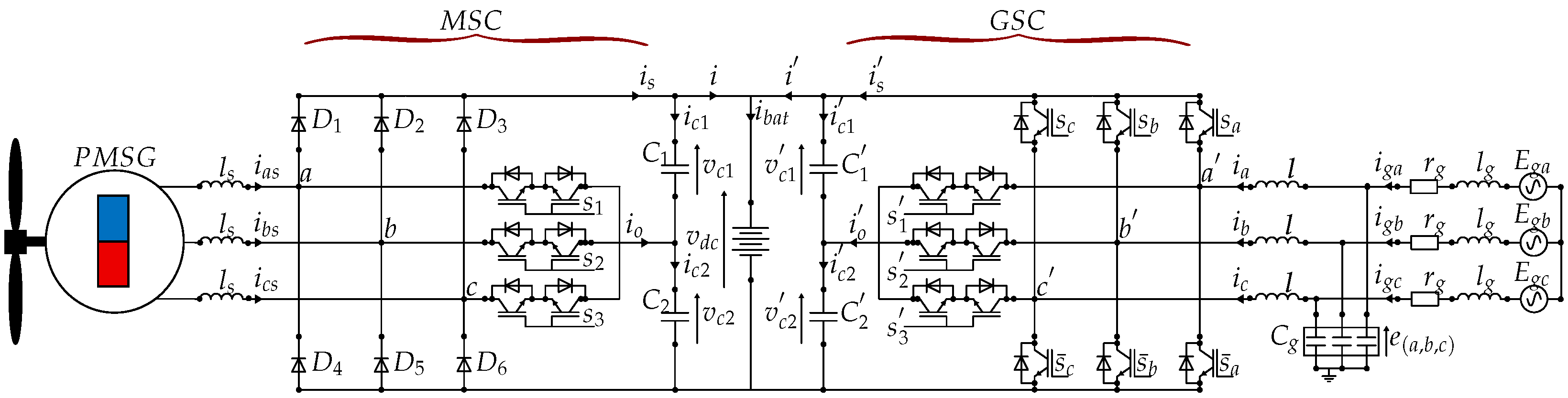
The objective of this work is to propose a promising approach for energy conversion and management aimed at efficiently integrating wind energy into the electrical grid. Specifically, the work focuses on the study of an energy conversion chain consisting of a synchronous aerogenerator, a Vienna rectifier, and a Li-ion storage battery, all coupled to the grid via a bidirectional Vienna rectifier. The schematic diagram of the studied system is presented in Figure 1.

The main objectives of this study are as follows:

• Mathematical Modeling: To better understand the system’s behavior and constraints.
• Definition of Control Objectives: Ensuring efficient energy conversion and stable interaction with the grid.
• Synthesis of Nonlinear Controllers: To improve the system’s dynamic performance and ensure better response to production and consumption variations.
• Development of an Energy Management Algorithm: Optimizing resource utilization while ensuring battery safety and durability.

This paper is organized as follows: Section 2 introduces the mathematical modeling of the system and offers a comprehensive overview of the suggested structure. In Section 3, the control strategy is developed, and stability aspects are thoroughly examined. The observer structure is introduced in Section 4, along with an examination of its convergence behavior. Section 5 centers on the development and implementation of the energy management system. Section 6 highlights and discusses the simulation results. Finally, Section 7 concludes the paper by summarizing the key findings.

2. System Modeling

2.1. The Three-Phase Grid Modeling

Through the application of the Park transformation and Kirchhoff’s laws, the following system of equations provides the mathematical description of the grid in (dq) coordinates [31]:

$$\begin{array}{cc}\hfill {\displaystyle \frac{d{i}_{gd}}{dt}}& =-{\displaystyle \frac{r_g}{l_g}}{i}_{gd}+{\omega }_g{i}_{gq}-{\displaystyle \frac{E_{gd}}{l_g}}+{\displaystyle \frac{e_d}{l_g}}\hfill \end{array}$$

(1a)

$$\begin{array}{cc}\hfill {\displaystyle \frac{d{i}_{gq}}{dt}}& =-{\displaystyle \frac{r_g}{l_g}}{i}_{gq}-{\omega }_g{i}_{gd}-{\displaystyle \frac{E_{gq}}{l_g}}\hfill \end{array}$$

(1b)

$$\begin{array}{cc}\hfill {\displaystyle \frac{d{e}_d}{dt}}& ={\displaystyle \frac{1}{C_g}}(i_{gd}-i_d)\hfill \end{array}$$

(1c)

$$\begin{array}{cc}\hfill {\displaystyle \frac{d{i}_d}{dt}}& =\begin{array}{c}\hfill -{\displaystyle \frac{r}{l}}{i}_d\end{array}+{\omega }_g{i}_q-{\displaystyle \frac{e_d}{l}}+{\displaystyle \frac{v_d}{l}}\hfill \end{array}$$

(1d)

$$\begin{array}{cc}\hfill \begin{array}{c}\hfill {\displaystyle \frac{d{i}_q}{dt}}\end{array}& =-{\displaystyle \frac{r}{l}}{i}_q-{\omega }_g{i}_d-{\displaystyle \frac{v_q}{l}}\hfill \end{array}$$

(1e)

where: ($i_{gd}$,$i_{gq}$) denote respectively the d-axis and q-axis components of the grid current; $l_g$ is the line grid’s inductance; $r_g$ is the grid’s equivalent resistance; ${\omega }_g$ is the grid’s angular frequency; $(E_{gd}$,$E_{gq})$ are, respectively, the grid voltage source components along the d-axis and q-axis; $e_d$ and $e_q$ are the components of the input converter voltage in the (d,q) coordinates; $C_g$ is the filter capacitance; $(r,l)$ is the filter resistance and inductance; $(i_d,i_q)$ are the direct and quadrature components of the converter’s input current; ($v_d$,$v_q$) are the $(v_a^{\prime },v_b^{\prime },v_c^{\prime })$ voltages in ($d,q$) coordinates.

2.2. The PMSG Model

The mathematical model of the synchronous wind turbine generator, in the (dq) coordinates, is given by the following system of equations [10]:

$$\begin{array}{cc}\hfill {\displaystyle \frac{d\Omega }{dt}}& =-{\displaystyle \frac{T_g}{J}}+{\displaystyle \frac{K_{em}}{J}}{i}_{sq}-{\displaystyle \frac{F}{J}}\Omega \hfill \end{array}$$

(2)

$$\begin{array}{cc}\hfill {\displaystyle \frac{d{i}_{sq}}{dt}}& =-{\displaystyle \frac{R_s}{L_s}}{i}_{sq}-p{\displaystyle \frac{{\Phi }_m}{L_s}}\Omega -p{i}_{sd}\Omega +{\displaystyle \frac{v_{sq}}{L_s}}\hfill \end{array}$$

(3)

$$\begin{array}{cc}\hfill {\displaystyle \frac{d{i}_{sd}}{dt}}& =-{\displaystyle \frac{R_s}{L_s}}{i}_{sd}+p\Omega i_{sq}+{\displaystyle \frac{v_{sd}}{Ls}}\hfill \end{array}$$

(4)

($i_{sd},i_{sq}$) and ($v_{sd},v_{sq}$) represent the averaged values of the stator current and voltage in the ($d-q$) reference frame, respectively. ${\varphi }_m$ represents the amplitude of magnetic flux generated by the rotor magnets. $L_s$ and $R_s$ correspond to the stator inductance and resistance. J, F, and p represent the total rotor inertia, the viscous friction coefficient, and the number of poles, respectively. $\Omega$ denotes the rotor speed, while $T_g$ represents the aerodynamic torque. Finally, the electromotive force constant is given by $K_{em}=(3/2)p{\varphi }_m$.

2.3. Vienna Rectifier and Bidirectional Vienna Converter Modeling

The structure of the bidirectional Vienna converter, as shown in Figure 1, consists primarily of six IGBTs with diodes connected in anti-parallel, arranged in a bridge configuration [32,33].

The dynamic of the DC output voltage ($v_{dc}$) on the Grid side converter is expressed by:

$${\displaystyle \frac{d{\left(v_{dc}\right)}^2}{dt}}={\displaystyle \frac{1}{C_0}}(v_d{i}_d+v_q{i}_q-v_{dc}{i}^{\prime })$$

(5)

with: $C_0={\displaystyle \frac{C}{4}}$.

The principle of power conservation results in the following equation:

$$v_d{i}_d+v_q{i}_q=e_d{i}_d-r(i_d^2+i_q^2)$$

(6)

By combining Equations (5) and (6), the state equation of the DC voltage is:

$${\displaystyle \frac{d{\left(v_{dc}\right)}^2}{dt}}={\displaystyle \frac{1}{C_0}}(e_d{i}_d-r(i_d^2+i_q^2)-v_{dc}{i}^{\prime })$$

(7)

Using the same method, we can show that the DC voltage’s dynamics, on the Vienna rectifier side, can be expressed as follows:

$${\displaystyle \frac{d{\left(v_{dc}\right)}^2}{dt}}={\displaystyle \frac{1}{C_0}}(K_{em}{i}_{sq}\Omega -R_s(i_{sd}^2+i_{sq}^2)-v_{dc}i)$$

(8)

Knowing that $i_{bat}=i+i^{\prime }$, and by combining (7) with (8), we can deduce that the dynamics of the DC voltage $v_{dc}$ can be written as follows:

$${\displaystyle \frac{d{\left(v_{dc}\right)}^2}{dt}}={\displaystyle \frac{1}{2C_0}}\left[K_{em}{i}_{sq}\Omega +e_d{i}_d-R_s(i_{sd}^2+i_{sq}^2)-r_g(i_{gd}^2+i_{gq}^2)-v_{dc}{i}_{bat}\right]$$

(9)

2.4. Battery System Modeling

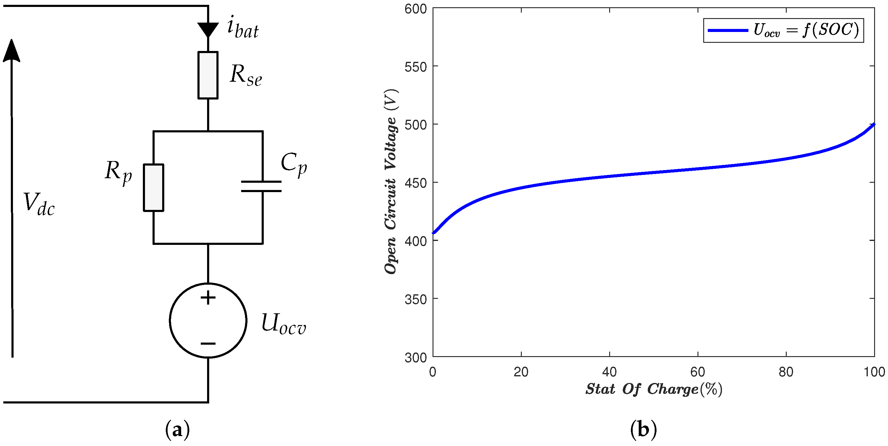
The battery energy storage system (BESS) is represented using a first-order Thevenin equivalent model because it provides a good compromise between modeling simplicity and dynamic accuracy. As depicted in Figure 2a, this model consists of an open-circuit voltage source $U_{ocv}$, a series internal resistance $R_{se}$, and a parallel $RC$ network $(R_p,C_p)$ used to capture the transient polarization effect of the battery. The open-circuit voltage $U_{ocv}$ is a nonlinear function of the battery state of charge (SOC). In this work, this relationship is approximated by the polynomial expression:

$$U_{ocv}={\gamma }_0+{\gamma }_{1}SOC+{\gamma }_{2}SO{C}^2+\dots +{\gamma }_{n}SO{C}^n$$

(10)

where the coefficients $({\gamma }_0,{\gamma }_1,\dots ,{\gamma }_n)$, presented in

Table 1. Coefficients of polynomial function $F(•)$.

${\mathit{\gamma }}_3$	${\mathit{\gamma }}_2$	${\mathit{\gamma }}_1$	${\mathit{\gamma }}_0$
$1.6656\times {10}^{-9}$	$-6.6816\times {10}^{-6}$	$0.0316$	$11.1033$

, are identified from the battery characteristic curve. The dynamic behavior of the polarization voltage $v_p$ is governed by:

$${\displaystyle \frac{d{v}_p}{dt}}={\displaystyle \frac{R_{se}+R_p}{C_p{R}_p}}{i}_{bat}+{\displaystyle \frac{U_{ocv}}{R_p{C}_p}}-{\displaystyle \frac{v_{dc}}{R_p{C}_p}}$$

(11)

while the battery current is given by:

$$i_{bat}={\displaystyle \frac{v_{dc}-v_p-U_{ocv}}{R_{se}}}$$

(12)

These equations show that the battery current depends on the difference between the DC-bus voltage, the open-circuit voltage, and the polarization voltage. Consequently, the battery exchanges power with the DC bus according to:

$$P_{bat}=v_{dc}{i}_{bat}$$

(13)

This relation makes it possible to explicitly interpret the charging and discharging dynamics of the BESS within the proposed energy conversion system. A positive value of $i_{bat}$ corresponds to battery charging, whereas a negative value indicates battery discharging. Therefore, the BESS power dynamics are directly linked to the DC-bus regulation and to the operating mode selected by the energy management strategy.

2.5. The System’s Model

The previously derived state-space equations are integrated to construct a comprehensive model representing the WECS shown in Figure 1. As a result, the unified model is formulated as follows:

$$\begin{array}{cc}\hfill {\dot{x}}_1& =-{\displaystyle \frac{T_g}{J}}+{\displaystyle \frac{K_{em}}{J}}{x}_2-{\displaystyle \frac{F}{J}}{x}_1\hfill \end{array}$$

(14a)

$$\begin{array}{cc}\hfill {\dot{x}}_2& =-{\displaystyle \frac{R_s}{L_s}}{x}_2-p{\displaystyle \frac{{\Phi }_m}{L_s}}{x}_1-p{x}_3{x}_1+{\displaystyle \frac{\sqrt{x_4}}{2L_s}}{u}_q\hfill \end{array}$$

(14b)

$$\begin{array}{cc}\hfill {\dot{x}}_3& =-{\displaystyle \frac{R_s}{L_s}}{x}_3+p{x}_1{x}_2+{\displaystyle \frac{\sqrt{x_4}}{2Ls}}{u}_d\hfill \end{array}$$

(14c)

$$\begin{array}{cc}\hfill {\dot{x}}_4& ={\displaystyle \frac{1}{2C_0}}\left[K_{em}{x}_1{x}_2+x_8{x}_9-R_s(x_2^2+x_3^2)-r_g(x_6^2+x_7^2)-\sqrt{x_4}{i}_{bat}\right]\hfill \end{array}$$

(14d)

$$\begin{array}{cc}\hfill {\dot{x}}_5& =a{i}_{bat}-b{x}_4+b{U}_{ocv}\hfill \end{array}$$

(14e)

$$\begin{array}{cc}\hfill {\dot{x}}_6& =-{\displaystyle \frac{r_g}{l_g}}{x}_6+{\omega }_g{x}_7+{\displaystyle \frac{E_{gd}}{l_g}}-{\displaystyle \frac{x_8}{l_g}}\hfill \end{array}$$

(14f)

$$\begin{array}{cc}\hfill {\dot{x}}_7& =-{\displaystyle \frac{r_g}{lg}}{x}_7-{\omega }_g{x}_6+{\displaystyle \frac{E_{gq}}{l_g}}\hfill \end{array}$$

(14g)

$$\begin{array}{cc}\hfill {\dot{x}}_8& ={\displaystyle \frac{1}{C_g}}(x_6-x_9)\hfill \end{array}$$

(14h)

$$\begin{array}{cc}\hfill {\dot{x}}_9& =-{\displaystyle \frac{r}{l}}{x}_9+{\omega }_g{x}_{10}+{\displaystyle \frac{x_8}{l}}-{\displaystyle \frac{\sqrt{x_4}}{2l}}{u}_d^{\prime }\hfill \end{array}$$

(14i)

$$\begin{array}{cc}\hfill {\dot{x}}_{10}& =-{\displaystyle \frac{r}{l}}{x}_{10}-{\omega }_g{x}_9-{\displaystyle \frac{\sqrt{x_4}}{2l}}{u}_q^{\prime }\hfill \end{array}$$

(14j)

where: $x_1,x_2,x_3,x_4,x_5,x_6$, $x_7$, $x_8$, $x_9$ and $x_{10}$ are, respectively, the averages values of $\Omega$, $i_{sq}$, $i_{sd}$, $v_{dc}^2$, $v_p$, $i_{gd}$, $i_{gq}$, $e_d$, $i_d$ and $i_q$.

3. Controller Design

3.1. Control Objectives

Based on the developed model (14a)–(14j), this section focuses on designing a nonlinear controller to achieve the following control objectives. The key point is that these objectives are dynamically adjusted according to the AC grid state, the SOC of the battery and the wind energy power. Consequently, the controller is required to switch between multiple operating modes, which will be detailed in a subsequent section.

CO1. CV1 mode enforced by the Machine side converter (MSC): When the battery’s state of charge reaches its nominal value, the regulator switches to mode CV1. Here, the converter keeps the battery voltage at a constant value $v_{dc}=v_{dc-max}$ to prevent overvoltage. The charging current gradually decreases as the battery approaches its full capacity, ensuring a safe and complete charge.

CO2. MPPT mode enforced by the MSC: This regulator acts on the wind turbine (via the unidirectional Vienna rectifier) to extract the maximum power from the wind. It continuously adjusts the control parameters (torque and rotational speed) to ensure that the wind turbine operates at its optimal efficiency point. The MPPT ensures that the wind turbine provides as much energy as possible to the converters and the battery, while staying within the system’s safety limits.

CO3. The d-axis current ($i_{sd}$) regulation enforced by the MSC: The regulator controlling the Vienna rectifier has two control outputs. The first ensures either the MPPT mode or the CV1 mode, while the second is reserved for the third control objective. In this objective, the regulator must cancel the direct component of the stator current $i_{sd}$, associated with the magnetic flux, in order to maximize torque and minimize losses.

CO4. CC2 mode enforced by the grid side converter (GSC): If the battery’s state of charge has not yet reached its maximum value, and the grid state indicates an excess of injected power, CC2 mode imposes a fixed current to recharge the battery ($i_{b-ref}=i_{bmax}$) from the grid, while limiting the current to protect the battery.

CO5. The quadratic grid current regulation enforced by the GSC: The goal of this control objective is to regulate the quadratic component of the grid current, to its reference $i_{q-ref}$, to improve the quality of the electrical power, reduce transmission losses, and maximize the utilization of the grid’s capacity.

CO6. Active power regulation enforced by the GSC: This control objective involves maintaining or adjusting the production and consumption of energy to stabilize the frequency and meet demand. More specifically, it aims to control the active power flow so that the electrical grid remains balanced despite variations in load or generation.

CO7. Reactive power regulation enforced by the GSC: The controller should ensure that the reactive power tracks its reference value, determined based on the energy needs of the grid, to ensure the quality of the power supply and the stability of the grid.

3.2. The DC Voltage Regulation (CV1 Mode)

Once the battery reaches its full state of charge ($SOC=100\%$), this control objective aims to force the DC voltage ($v_{dc}$) to track the reference $v_{dc-ref}=\begin{array}{c}\hfill \sqrt{x_4^{*}}\end{array}=500$ V. Using the sliding mode approach, by considering the tracking error $e_1=x_4-x_4^{*}$, and the first sliding surface as follow:

$$s_1=e_1+c_1{\int }_0^t{e}_1\left(\tau \right)d\tau ;c_1>0$$

(15)

Taking into account (14d) and (15), the dynamic of the sliding surface (15) using the virtual input $U_{v1}=x_2$ yields:

$${\dot{s}}_1={\chi }_1(x,t)+{\displaystyle \frac{1}{2C_0}}{K}_{em}{x}_1{U}_{v1}$$

(16)

where:

$${\chi }_1(x,t)={\displaystyle \frac{1}{2C_0}}[x_8{x}_9-R_s(x_2^2+x_3^2)-r_g(x_6^2+x_7^2)-\sqrt{x_4}{i}_{bat}]+c_1{x}_4-c_1{x}_4^{*}-{\dot{x}}_4^{*}$$

(17)

Using the Lyapunov function $v_1=0.5s_1^2$, which may be written as follows, the control input $U_{v1}^{*}$ is aimed at controlling the DC voltage:

$$U_{v1}^{*}=-{\displaystyle \frac{2C_0}{K_{em}{x}_1}}\left({\chi }_1(x,t)+{\beta }_1\mathrm{sign}\left(s_1\right)\right);{\beta }_1>0$$

(18)

Let’s define a new control tracking error $e_2=U_{v1}-U_{v1}^{*}$, taking into account (14b). The following equation gives its time derivative:

$${\dot{e}}_2=-{\displaystyle \frac{R_s}{L_s}}{x}_2-p{\displaystyle \frac{{\varphi }_m}{L_s}}{x}_1-p{x}_3{x}_1-{\dot{U}}_{v1}^{*}+{\displaystyle \frac{\sqrt{x_4}}{2L_s}}(U_{q-eq}+U_{q-sw})$$

(19)

A first-order sliding surface can be expressed as:

$$s_2=e_2+c_2{\int }_0^t{e}_2\left(\tau \right)d\tau ;c_2>0$$

(20)

Differentiating Equation (20) with respect to time yields:

$${\dot{s}}_2={\chi }_2(x,t)+{\displaystyle \frac{\sqrt{x_4}}{2L_s}}(U_{q-eq}+U_{q-sw})$$

(21)

with:

$${\chi }_2(x,t)=-{\displaystyle \frac{R_s}{L_s}}{x}_2-p{\displaystyle \frac{{\varphi }_m}{L_s}}{x}_1-p{x}_1{x}_3+c_2{x}_2-c_2{U}_{v1}^{*}-{\dot{U}}_{v1}^{*}$$

(22)

One way to express the equivalent control input is:

$$U_{q-eq}={\displaystyle \frac{-2L_s}{\sqrt{x_4}}}{\chi }_2(x,t)$$

(23)

Given the dynamics $\left({\dot{v}}_2\right)$ of the Lyapunov function $v_2=0.5s_2^2$. The formula for the battery voltage control input is as follows:

$$U_{q-CV1}=-{\displaystyle \frac{2L_s}{\sqrt{x_4}}}\left({\chi }_2(x,t)+{\beta }_{2}sign\left(s_2\right)\right);{\beta }_2>0$$

(24)

3.3. The MPPT Mode Controller

3.3.1. Reference Speed Optimizer

The development of a speed reference optimizer for MPPT in wind turbines using neural networks is a promising approach to improving energy efficiency. Traditional MPPT methods often rely on fixed algorithms that may not adapt well to varying wind conditions. By integrating neural networks, the optimizer can learn from historical and real-time data to dynamically adjust the speed reference, ensuring optimal power extraction. This intelligent system enhances the turbine’s responsiveness to fluctuations in wind speed, reducing energy losses and increasing overall performance. Moreover, neural networks can handle nonlinearity and uncertainties in wind energy systems, making them a robust solution for MPPT optimization [34].

3.3.2. Speed Regulation for Synchronous Aerogenerator:

The MPPT mode is responsible for transferring the maximum available wind power to the battery and grid through the Vienna converters. To this end, the rotor speed $\Omega$ must track the optimal reference speed ${\Omega }_{ref}$, generated by the neural network optimizer.

Now, let us define the rotor speed tracking error $e_3=\Omega -{\Omega }_{ref}$, and the sliding surface:

$$s_3=e_3+c_3{\int }_0^t{e}_3\left(\tau \right)d\tau ;c_3>0$$

(25)

By differentiating the aforementioned sliding surface and introducing the virtual input $U_{v3}=x_2$, the following expression is obtained:

$${\dot{s}}_3={\chi }_3(x,t)+{\displaystyle \frac{K_{em}}{J}}{U}_{v3}$$

(26)

where:

$${\chi }_3(x,t)=-{\displaystyle \frac{T_g}{J}}-{\displaystyle \frac{F}{J}}{x}_1+c_3{x}_1-{\dot{x}}_1^{*}-c_3{x}_1^{*}$$

(27)

Using the Lyapunov function candidate $v_3=0.5s_3^2$, the virtual control input can be formulated as follows:

$$U_{v3}^{*}=-{\displaystyle \frac{J}{K_{em}}}({\chi }_3(x,t)+{\beta }_{3}sign\left(s_3\right));{\beta }_3>0$$

(28)

the virtual tracking error is defined as: $e_4=U_{v3}-U_{v3}^{*}$, in view of (14b), its time derivative is given by:

$${\dot{e}}_4=-{\displaystyle \frac{R_s}{L_s}}{x}_2-p{\displaystyle \frac{{\varphi }_m}{L_s}}{x}_1-p{x}_1{x}_3+{\displaystyle \frac{\sqrt{x_4}}{2L_s}}(U_{q-eq}+U_{q-sw})$$

(29)

Now let us consider the sliding surface:

$$s_4=e_4+c_4{\int }_0^t{e}_4\left(\tau \right)d\tau ;c_4>0$$

(30)

the dynamic of (30) yields:

$${\dot{s}}_4={\chi }_4(x,t)+{\displaystyle \frac{\sqrt{x_4}}{2L_s}}(U_{q-eq}+U_{q-sw})$$

(31)

where:

$${\chi }_4=-{\displaystyle \frac{R_s}{L_s}}{x}_2-p{\displaystyle \frac{{\varphi }_m}{L_s}}{x}_1-p{x}_1{x}_3+c_4{x}_2-c_4{U}_{v3}^{*}-{\dot{U}}_{v3}^{*}$$

(32)

Using the results from (29) and (31), the expression of the equivalent control input becomes:

$$U_{q-eq}=-{\displaystyle \frac{2L_s}{\sqrt{x_4}}}{\chi }_4(x,t)$$

(33)

The Lyapunov function $v_4$ can be chosen as $v_4=0.5s_4^2$, the speed control law $U_{q-mppt}$ is given by:

$$U_{q-mppt}=-{\displaystyle \frac{2L_s}{\sqrt{x_4}}}({\chi }_4(x,t)+{\beta }_{4}sign\left(s_4\right));{\beta }_4>0$$

(34)

3.4. The D-Axis Current Controller

The aim is to regulate the current $x_3=i_{sd}$, to a reference value $x_3^{*}=i_{sd-ref}=0$. To fulfill this control objective, consider the tracking error $e_5=x_3-x_3^{*}$, and the following sliding surface:

$$s_5=e_5+c_5{\int }_0^t{e}_5\left(\tau \right)d\tau ;c_5>0$$

(35)

In view of (14c), the time derivative of (35) is given by:

$${\dot{s}}_5={\chi }_5(x,t)+{\displaystyle \frac{\sqrt{x_4}}{2L_s}}(U_{d-eq}+U_{d-sw})$$

(36)

where:

$${\chi }_5=-{\displaystyle \frac{R_s}{L_s}}{x}_3+p{x}_1{x}_2+c_5{x}_3$$

(37)

The equivalent control input can be written as:

$$U_{d-eq}=-{\displaystyle \frac{2L_s}{\sqrt{x_4}}}{\chi }_5(x,t)$$

(38)

Now we chose the Lyapunov function $v_5=0.5s_5^2$, taking the derivative of $v_5$, the d-axis control input is given by:

$$U_d=-{\displaystyle \frac{2L_s}{\sqrt{x_4}}}({\chi }_5(x,t)+{\beta }_{5}sign\left(s_5\right));{\beta }_5>0$$

(39)

Proposition 1.

Consider the subsystem defined by (14a), (14c) and (14d), Given the control inputs (24), (34) and (39), and the sliding surfaces (20), (30) and (35), where $(c_i,{\beta }_i)$ are positive design parameters. There exists a Lyapunov function $V_{f1}=0.5{\sum }_{i=1}^5{s}_i^2$ such that:

$${\dot{V}}_{f1}=\sum _{i=1}^5{s}_i{\dot{s}}_i\le -{\mu }_1\sqrt{V_{f1}};with{\mu }_1=min\left({\beta }_i\right)$$

(40)

The finite-time convergence of the closed loop system consequently satisfies the following inequality for any beginning trajectory:

$$T\left(t_0\right)\le 2{\displaystyle \frac{\sqrt{V_{f1}}}{{\mu }_1}}$$

(41)

Proof. 

Take into account the Lyapunov function:

$$V_{f1}=0.5\sum _{i=1}^5{s}_i^2$$

(42)

The dynamic of (42) is given by:

$${\dot{V}}_{f1}=\sum _{i=1}^5{s}_i{\dot{s}}_i$$

(43)

Replacing (18), (24), (28), (34) and (39), respectively, in (16), (21), (26), (31) and (36), the expression (43) yields:

$${\dot{V}}_{f1}=-\sum _{i=1}^5{s}_i\left({\beta }_{i}sign\left(s_i\right)\right)⩽-\sum _{i=1}^5{\beta }_i\left|s_i\right|$$

(44)

by applying the inequality: $0⩽r⩽2$

$${\left(\sum _{i=1}^n{x}_i^2\right)}^{{\displaystyle \frac{r}{2}}}⩽\sum _{i=1}^n{\left|x_i\right|}^r$$

(45)

Inequality (43) becomes:

$${\dot{V}}_{f1}⩽-{\mu }_1\sqrt{V_{f1}}$$

(46)

By integrating (46), the following inequality is obtained:

$$\sqrt{V_{f1}}⩽-{\displaystyle \frac{1}{2}}{\mu }_{1}t+\sqrt{V_{f1}\left(t_0\right)}$$

(47)

The designed controllers ensure the system’s convergence properties, with the the closed-loop’s convergence time is expressed as follows:

$$T\left(t_0\right)⩽2{\displaystyle \frac{\sqrt{V_{f1}\left(t_0\right)}}{{\mu }_1}}$$

(48)

This ends proof of Proposition 1. □

3.5. Control of Battery Charging Current

This section focuses on ensuring that the designed controller compels the current $i_{bat}$ to follow its predetermined reference $i_{bat}^{*}=i_{bat-max}$. We define the current error as: $e_6=i_{bat}-i_{bat}^{*}$.

$$i_{bat}={\displaystyle \frac{1}{R_{se}}}(\sqrt{x_4}-x_7-U_{ocv})$$

(49)

To achieve system stabilization using the virtual control input $U_{v6}=x_9$, the following sliding surface is considered:

$$s_6=e_6+c_6{\int }_0^t{e}_6\left(\tau \right)d\tau ;c_6>0$$

(50)

The dynamic of (50) yields the following equation:

$$\dot{s_6}={\chi }_6(x,t)+{\displaystyle \frac{1}{4R_{se}{C}_0\sqrt{x_4}}}{x}_8(U_{v6-eq}+U_{v6-sw})$$

(51)

where

$$\begin{array}{cc}\hfill {\chi }_6(x,t)=& {\displaystyle \frac{1}{4R_{se}{C}_0\sqrt{x_4}}}\left(K_{em}{x}_1{x}_2-R_s(x_2^2+x_3^2)-r_g(x_6^2+x_7^2)-\sqrt{x_4}{i}_{bat}\right)\hfill \\ \hfill & -{\displaystyle \frac{1}{R_{se}}}\left(-{\displaystyle \frac{r_g}{l_g}}{x}_7-{\omega }_g{x}_6+{\displaystyle \frac{E_{gq}}{l_g}}\right)+c_6{i}_{bat}-{\dot{i}}_{bat}^{*}-c_6{i}_{bat}^{*}.\hfill \end{array}$$

(52)

Using the Lyapunov function $v_6=0.5s_6^2$, the following virtual control input can be derived:

$$U_{v6}^{*}=-{\displaystyle \frac{4}{x_8}}{R}_{se}{C}_0\sqrt{x_4}({\chi }_6(x,t)+{\beta }_{6}sign\left(s_6\right));{\beta }_6>0$$

(53)

To ensure system stabilization, the virtual control regulation error is defined as $e_7=U_{v6}-U_{v6}^{*}$, along with the formulation of the sliding surface:

$$s_7=e_7+c_7{\int }_0^t{e}_7\left(\tau \right)d\tau ;c_7>0$$

(54)

the dynamic of (54) undergoes:

$$\dot{s_7}={\chi }_7(x,t)+{\displaystyle \frac{\sqrt{x_4}}{2l}}(U_{d-eq}+U_{d-sw})$$

(55)

where

$${\chi }_7(x,t)=-{\displaystyle \frac{r}{l}}{x}_9+{\omega }_g{x}_{10}+{\displaystyle \frac{x_8}{l}}+c_7{x}_9-{\dot{U}}_{v6}^{*}-c_7{U}_{v6}^{*}$$

(56)

In light of Equation (55), the equivalent control law can be derived as follows:

$$u_{d-eq}=-{\displaystyle \frac{2l}{\sqrt{x_4}}}{\varphi }_7(x,t)$$

(57)

A Lyapunov function can be selected as $v_7=0.5s_7^2$. Analyzing the dynamics of $v_7$, it leads to the following control input for regulating the charging current:

$$U_{d-i_{bat}}^{\prime }=-{\displaystyle \frac{2l}{\sqrt{x_4}}}({\chi }_7(x,t)+{\beta }_{7}sign\left(s_7\right));{\beta }_7>0$$

(58)

3.6. Quadrature Current Control

The aim of this control objective is to regulate the q-axis current, $i_q=x_{10}$, towards its reference value of $x_{10}^{*}=0$. To facilitate this, the tracking error is defined as $e_8=x_{10}-x_{10}^{*}$, and the corresponding sliding surface is expressed as follows:

$$s_8=e_8+c_8{\int }_0^t{e}_8\left(\tau \right)d\tau ;c_8>0$$

(59)

By incorporating (14j), the time derivative of (59) is determined as follows:

$${\dot{s}}_8={\chi }_8(x,t)-{\displaystyle \frac{\sqrt{x_4}}{2l}}(U_{q-eq}+U_{q-sw})$$

(60)

where:

$${\chi }_8(x,t)=-{\displaystyle \frac{r}{l}}{x}_{10}-w_g{x}_9-{\dot{x}}_{10}^{*}+c_8{x}_{10}-c_8{x}_{10}^{*}$$

(61)

Referring to (60), the equivalent control law is defined as:

$$U_{q-eq}={\displaystyle \frac{2L}{\sqrt{x_4}}}{\chi }_8(x,t)$$

(62)

To achieve stabilization of the $i_q$ loop, we propose the Lyapunov function $v_8=0.5s_8^2$. The time derivative of $v_8$ becomes a negative definite function when the control input $U_{q-sw}$ is selected as follows:

$$U_{q-sw}={\displaystyle \frac{2l}{\sqrt{x_4}}}(-{\beta }_{8}sign\left(s_8\right));{\beta }_8>0$$

(63)

Based on (62) and (63), the control law can be expressed as follows:

$$U_{q-axis}^{\prime }={\displaystyle \frac{2l}{\sqrt{x_4}}}({\chi }_8(x,t)-{\beta }_{8}sign\left(s_8\right))$$

(64)

The subsystem governed by Equations (14d), (14e), and (14j). Utilizing the sliding surface functions defined in (50), (55), and (59), along with the control input given in (53), (58), and (64), and assuming all design parameters ($c_i,{\beta }_i$) are strictly positive, a Lyapunov function $V_{f2}=0.5{\sum }_{i=6}^8{s}_i^2$ can be established, ensuring that:

$$\begin{array}{c}\hfill {\dot{V}}_{f2}=\sum _{i=6}^8{s}_i{\dot{s}}_i⩽-{\mu }_2\sqrt{V_{f2}};with{\mu }_2=min\left({\beta }_i\right)\end{array}$$

(65)

The closed-loop dynamics lead to finite-time convergence, validated through the following inequality:

$$T\left(t_0\right)⩽2{\displaystyle \frac{\sqrt{V_{f2}\left(t_0\right)}}{{\mu }_2}}$$

(66)

3.7. Active Power Control:

The proposed controller is designed to maintain the consumed active power in close alignment with a reference value, $P^{*}$. To accomplish this, we define the tracking error as $e_9=P-P^{*}=x_8{x}_9-P^{*}$. By applying the integral sliding mode method, we select the sliding surface:

$$s_9=e_9+c_9{\int }_0^t{e}_9\left(\tau \right)d\tau ;c_9>0$$

(67)

Taking into account (14h) and (14i), the time derivative of (67) can be expressed as follows:

$$\dot{s_9}={\chi }_9(x,t)+x_8{\displaystyle \frac{\sqrt{x_4}}{2l}}(U_{d-eq}+U_{d-sw})$$

(68)

where

$$\begin{array}{cc}\hfill {\chi }_9(x,t)=& {\displaystyle \frac{x_9}{C_g}}(x_6-x_9)+x_8(-{\displaystyle \frac{r}{l}}{x}_9+{\omega }_g{x}_{10}+{\displaystyle \frac{x_8}{l}})+c_9{x}_8{x}_9-c_9{P}^{*}-{\dot{P}}^{*}\hfill \end{array}$$

(69)

The equivalent control law $U_{d-eq}$ can be determined from Equation (68):

$$U_{d-eq}=-{\displaystyle \frac{2l}{x_8\sqrt{x_4}}}{\chi }_9(x,t)$$

(70)

We propose the Lyapunov function $v_9=0.5s_9^2$. To ensure that ${\dot{v}}_9$ remains negative definite, the discontinuous control input $U_{d-sw}$ is selected as follows:

$$U_{d-sw}=-{\displaystyle \frac{2l}{x_8\sqrt{x_4}}}\left({\beta }_{9}sign\left(s_9\right)\right);{\beta }_9>0$$

(71)

By combining Equations (70) and (71), we derive the integral control input for the active power loop as follows:

$$U_{d-p}^{″}=-{\displaystyle \frac{2l}{x_8\sqrt{x_4}}}({\chi }_9(x,t)+{\beta }_{9}sign\left(s_9\right))$$

(72)

3.8. The Reactive Power Regulation

A controller is designed that drives the power Q to track its reference value $Q^{*}$. The error is defined as $e_{10}=Q-Q^{*}=x_8{x}_{10}-Q^{*}$, and the corresponding sliding surface is established as follows:

$$s_{10}=e_{10}+c_{10}{\int }_0^t{e}_{10}\left(\tau \right)d\tau ;c_{10}>0$$

(73)

Utilizing (14h) and (14j), the dynamic of (73) results in:

$${\dot{s}}_{10}={\chi }_{10}(x,t)+(U_{q-eq}+U_{q-sw})$$

(74)

where:

$$\begin{array}{cc}\hfill {\chi }_{10}(x,t)=& {\displaystyle \frac{x_{10}}{C_g}}(x_6-x_9)+x_8(-{\displaystyle \frac{r}{l}}{x}_{10}-{\omega }_g{x}_9)+c_{10}{x}_8{x}_{10}-c_{10}{Q}^{*}-{\dot{Q}}^{*}\hfill \end{array}$$

(75)

Using Equation (74), the control law $U_{q-eq}$ can be expressed as follows:

$$U_{q-eq}=-{\displaystyle \frac{2l}{x_8\sqrt{x_4}}}{\chi }_{10}(x,t)$$

(76)

To regulate the reactive power, we consider the Lyapunov function candidate $v_{10}=0.5s_{10}^2$. It can be readily verified that its dynamic becomes a negative definite function when the discontinuous control input $U_{q-sw}$ is selected as follows:

$$U_{q-sw}=-{\displaystyle \frac{2l}{x_8\sqrt{x_4}}}\left({\beta }_{10}sign\left(s_{10}\right)\right);{\beta }_{10}>0$$

(77)

By combining (76) and (77), the integral sliding mode (ISM) control input for reactive power loop can be formulated as:

$$U_{q-Q}^{″}=-{\displaystyle \frac{2l}{x_8\sqrt{x_4}}}({\chi }_{10}(x,t)+{\beta }_{10}sign\left(s_{10}\right))$$

(78)

Proposition 2.

The dynamical behavior of the subsystem defined by the state Equations (14h), (14i), and (14j) can be analyzed through the proposed control framework. By implementing the integral sliding surfaces (67) and (73) in conjunction with the control inputs (72) and (78), and under the condition that all design parameters ($c_i$, ${\lambda }_i$) maintain positive values, the closed-loop system exhibits the following dynamic characteristics:

$$\begin{array}{cc}\hfill {\dot{e}}_9& =-{\lambda }_9\left|e_9\right|\hfill \end{array}$$

(79)

$$\begin{array}{cc}\hfill {\dot{e}}_{10}& =-{\lambda }_{10}\left|e_{10}\right|\hfill \end{array}$$

(80)

Regarding the Lyapunov function $V_{c1}=0.5s_9^2+0.5s_{10}^2$, The linear system in question is asymptotically and globally stable.

Proof. 

Expression (79) is derived from Equations (68), (71), and (72), while Equation (80) is gotten from (74), (77), and (78). These respectively result in the following:

$${\dot{V}}_{c1}=-{\lambda }_9{e}_9^2-{\lambda }_{10}{e}_{10}^2$$

(81)

The error system demonstrates global and asymptotic stability, as $\dot{V}c1$ is a negative definite function with respect to the state vector ($e_9,e_{10}$). Although the system is linear, achieving asymptotic stability inherently guarantees exponential stability. □

4. Adaptive Observer Design

Battery lifetime is a critical factor in energy storage systems, and protecting it from overcharging and deep discharge can significantly extend its lifespan. This underscores the importance of accurately estimating the SOC. However, as illustrated in Figure 2b, the correlation between the SOC and the $U_{ocv}$ exhibits nonlinear behavior. The inherent nonlinear relationship between SOC and terminal voltage ($V_{dc}$) introduces significant challenges in obtaining accurate SOC estimates through voltage measurements alone. To address this limitation, a nonlinear observer design incorporating both voltage and current measurements ($V_{dc}$, $i_{bat}$) can be employed to enhance SOC estimation accuracy. This approach leverages the complementary information from multiple measurements to overcome the observability constraints present in voltage-only estimation methods [35].

4.1. The Battery’S Dynamical Model

The compact form of the battery’s dynamic model is presented in the subsequent proposition.

Proposition 3.

Let us consider the state vector $\varphi ={[{\varphi }_1,{\varphi }_2,{\varphi }_3]}^T={[v_{dc},v_p,U_{ocv}]}^T$ and the battery system of Equations (9) and (11). Its the simplified form can be expressed as follows:

$$\left\{\begin{array}{cc}\hfill \dot{\varphi }& =A\varphi +\psi (h(x,t),{\varphi }_1))+D\zeta \left(t\right)\hfill \\ \hfill y& =C\varphi \hfill \end{array}\right.$$

(82)

The system matrices are specified as follows:

$$A=\left(\begin{array}{ccc}-k_1& k_1& k_1\\ 0& -k_2& -k_3\\ 0& 0& 0\end{array}\right) ; \Psi \left(t\right)=\left(\begin{array}{c}h(x,t)\\ k_3{\varphi }_1\\ 0\end{array}\right) ; D=\left(\begin{array}{c}0\\ 0\\ 1\end{array}\right);C=\left(\begin{array}{ccc}1& 0& 0\end{array}\right)$$

where, $k_1={\displaystyle \frac{1}{2C{R}_{se}}}$ ; $k_2={\displaystyle \frac{1}{C_p}}{\displaystyle \frac{R_p+R_{se}}{R_p{R}_{se}}}$; $k_3={\displaystyle \frac{1}{C_{p}Rse}}$.

The signal $h(x,t)$ represents the measured output, while $\zeta \left(t\right)$ denotes a bounded function characterized by the following properties:

$$\left|\zeta \left(t\right)\right|⩽{\zeta }_0$$

(83)

${\zeta }_0>0$ is a real constant.

Proof. 

Considering Equation (9), and the fact that the battery power is given by $P_{bat}=v_{dc}{i}_{bat}$ we can derive the following expression by combining (9) with (11):

$$\begin{array}{cc}\hfill {\displaystyle \frac{d{v}_{dc}}{dt}}& =-k_1{v}_{dc}+k_1{v}_p+k_1{U}_{ocv}+h(x,t)\hfill \end{array}$$

(84)

$$\begin{array}{cc}\hfill {\displaystyle \frac{d{v}_p}{dt}}& =k_3{v}_{dc}-k_2{v}_p-k_3{U}_{ocv}\hfill \end{array}$$

(85)

$$\begin{array}{cc}\hfill {\displaystyle \frac{d{U}_{ocv}}{dt}}& =\zeta \left(t\right)\hfill \end{array}$$

(86)

The battery’s state of charge and open-circuit voltage ($U_{ocv}$) exhibit a nonlinear relationship, with limited dynamics. This implies that:

$${\displaystyle \frac{d{U}_{ocv}}{dt}}=\zeta \left(t\right)$$

(87)

where, $\left|\zeta \left(t\right)\right|⩽{\zeta }_0$. □

4.2. Design Methodology for Battery Charge State Observation

The designed observer enables the estimation of the open-circuit voltage $U_{ocv}$. Utilizing the polynomial point-by-point interpolation technique (

Table 2. Observer parameters.

${\mathit{l}}_3$	${\mathit{l}}_2$	${\mathit{l}}_1$
150	120	100

), the following equation is derived to define the relationship between SOC and $U_{ocv}$.

$$SOC=f\left(U_{ocv}\right)={\alpha }_n{U}_{ocv}^n+{\alpha }_{n-1}{U}_{ocv}^{(n-1)}+\dots +{\alpha }_1{U}_{ocv}+{\alpha }_0$$

(88)

The coefficients of the polynomial function $f\left(x\right)$ are denoted as (${\alpha }_0,{\alpha }_1,\dots ,{\alpha }_n$).

Theorem 1.

Assuming the boundedness of $\zeta \left(t\right)$ such that $\parallel \zeta \left(t\right)\parallel ⩽{\zeta }_0$, and referring to the system in (82), the following results can be derived:

• The system presented below functions as an observer for (82). The gain ($L\in {\mathbb{R}}^3$) is selected to ensure that ($A-LC$) possesses eigenvalues with negative real parts, confirming its Hurwitz stability.

  $$\left\{\begin{array}{cc}\hfill \dot{\widehat{\varphi }}& =A\widehat{\varphi }+\psi (g(x,t),\widehat{{\varphi }_1}))-LC(\widehat{\varphi }-\varphi )\hfill \\ \hfill y& =C\widehat{\varphi }\hfill \end{array}\right.$$

  (89)
• Let ρ be an arbitrary positive real number, where $\rho >{\rho }_0$, and independent of the initial condition $z\left(t_0\right)$, there exist positive real constants $(n_1,n_2,n_3)$ ensuring that $z\left(t\right)=\widehat{\varphi }-\varphi$ exhibits global convergence and adheres to the following inequality:

  $$\parallel z\left(t\right)\parallel \le n_1\parallel z\left(t_0\right)\parallel e^{-n_2(t-t_0)}+{\displaystyle \frac{n_3}{n_2}}$$

  (90)

Hence, irrespective of the initial conditions, $z\left(t\right)$ will converge to a specific limit. Moreover, by selecting a sufficiently large value for ρ, the error can be minimized further.

Proof. 

The demonstration of the theorem is detailed in Section 4.2 of my previous article [32]. □

5. Energies Management System

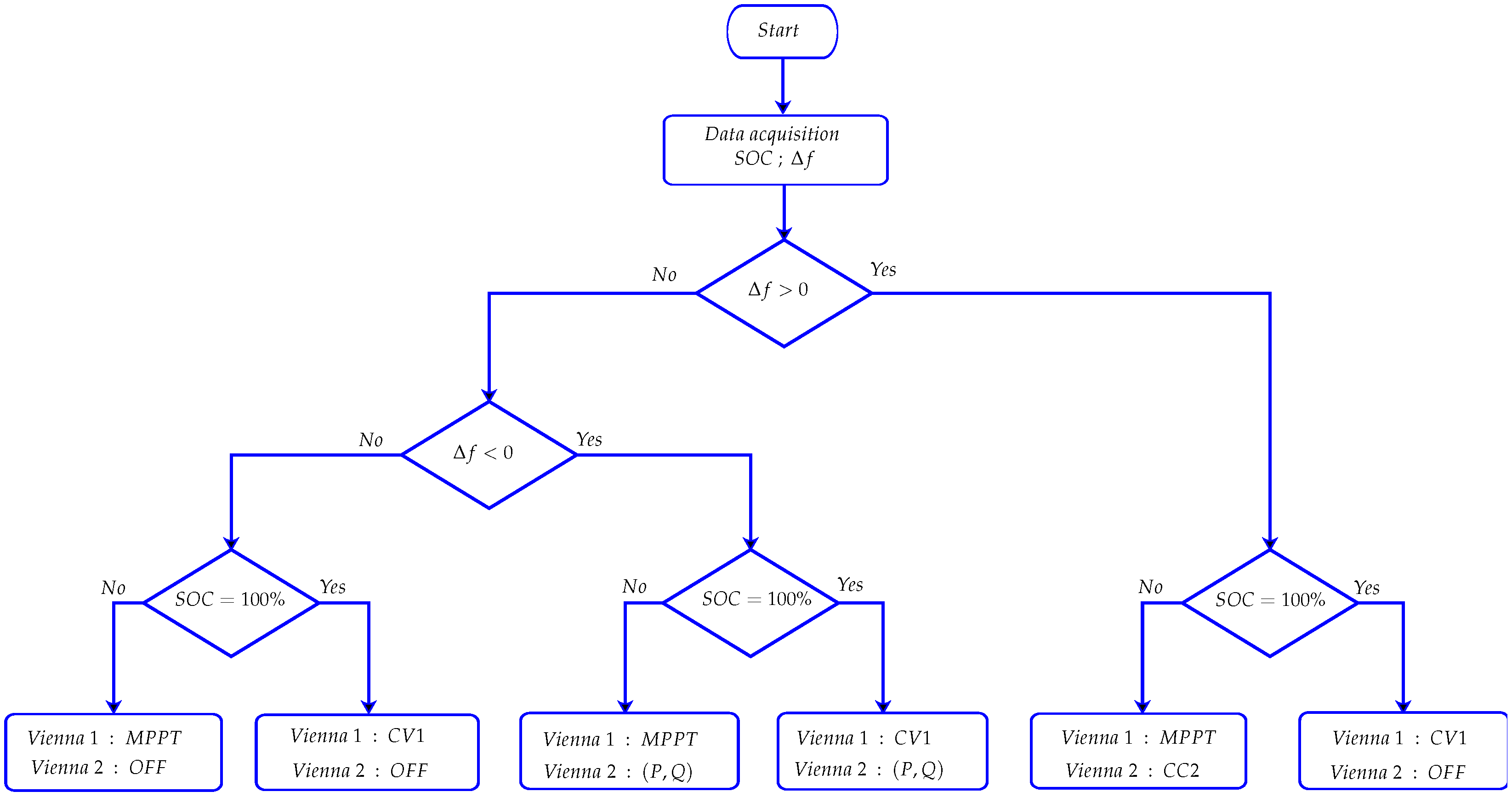
The studied energy conversion system is based on a synchronous wind generator connected to the electrical grid through a conversion architecture comprising two Vienna rectifiers: a unidirectional one (MSC) and a bidirectional one (GSC). The energy management algorithm, illustrated in Figure 3, aims to efficiently coordinate the various conditions. The energy management of this system relies on analyzing grid frequency variations ($\Delta f$) and the battery’s ($SOC$), enabling the adoption of the most appropriate operating mode.

When the grid frequency increases $(\Delta f>0)$, it indicates a surplus of injected power. Provided that the battery is not yet at 100% SOC, the MSC operates in MPPT mode, while the GSC operates in CC2 mode to limit the battery charging current to $i_{b-max}$. Conversely, if $SOC=100\%$, the MSC switches to CV1 mode, and the GSC disconnects (OFF) to avoid overcharging.

If the grid frequency decreases ($\Delta f<0$), it indicates a deficit of injected power. When the battery is partially charged, the MSC remains in MPPT mode to maximize wind power production, and the GSC continues to regulate grid power in $(P,Q)$ mode. If the battery reaches its maximum level $(SOC=100\%)$, the MSC switches to CV1 mode, while the GSC ensures the regulation of active and reactive power in the grid using $(P,Q)$ mode.

Finally, when the frequency is stable ($\Delta f=0$), the system adjusts its modes based on the battery’s state of charge: the MSC operates either in MPPT mode (if the battery is not full) or in CV1 mode (if the battery is charged), while the GSC remains disconnected from the grid ($OFF$).

This management scheme optimizes the utilization of wind energy while ensuring grid energy stability and efficient charging of the storage battery.

6. Simulation Result

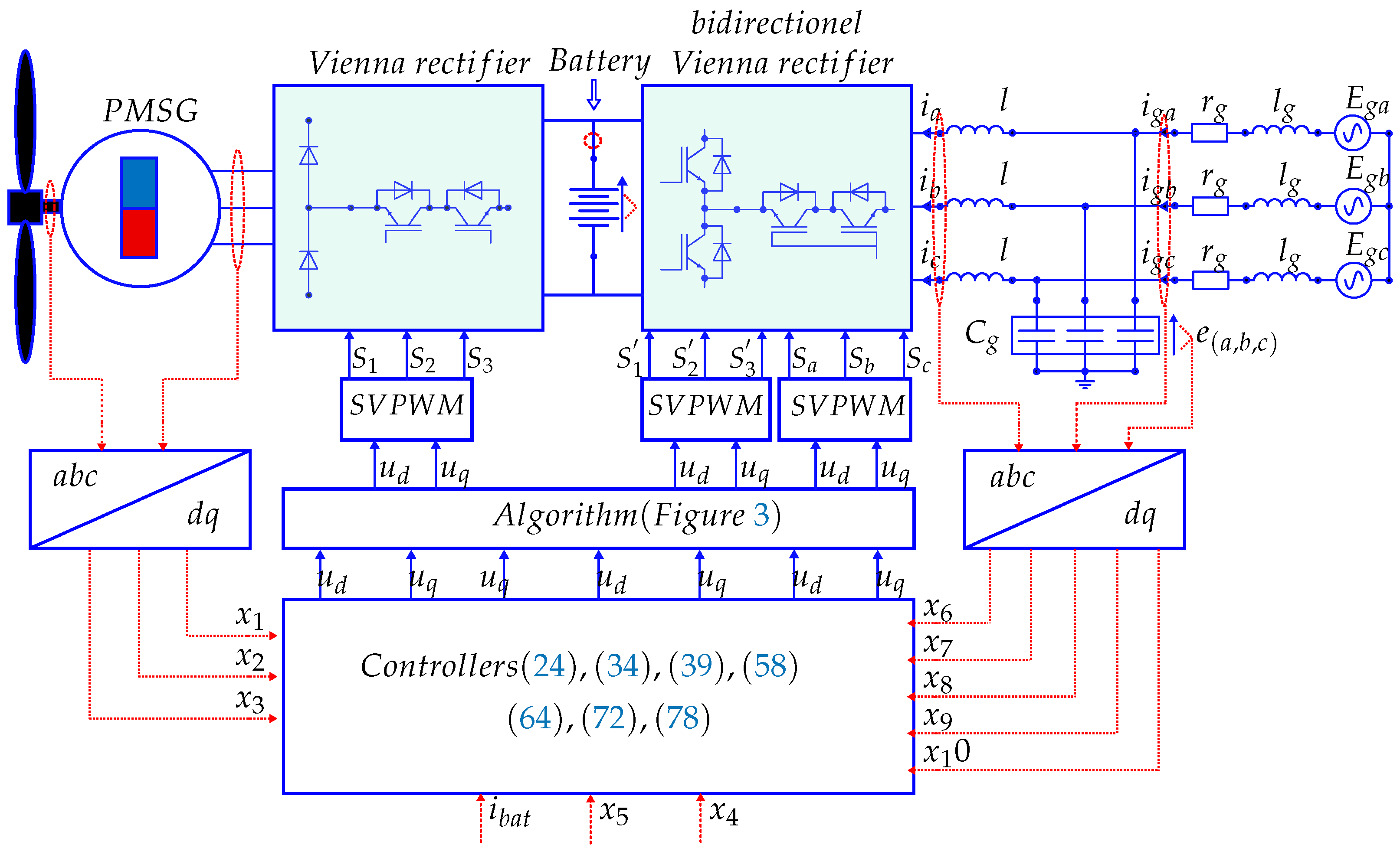
The simulation scheme is described in Figure 4. The controllers (24), (34), (39), (58), (64), (72), and (78), as well as the energy management algorithm (Figure 3), will be evaluated in the MATLAB/SIMULINK 2021 environment. The design parameters and the electromechanical characteristics of the simulated system are presented respectively in

Table 3. Simulation Parameters.

Characteristics	Values	Characteristics	Values
Wind Turbine		Power Line
Nominal Power	$P_t=25$ KW	Line Resistance	$r_g=0.6\Omega$
Rotor Radius	$R_t=6.5$ m	Line Inductance	$l_g=0.009$ H
Blade Pitch Angle	β = 2°	LC Filter
Aerogenerator	Filter Inductance	$l=0.001$ H
Nominal Power	$P_n=25$ KW	Filter Capacitance	$C_g=470$ uF
Number of Pole Pairs	$p=6$	Li-ion Battery
Nominal Speed	${\Omega }_n=60$ rad/s	Internal Resistance	$R_{se}=0.05\Omega$
Stator Resistance	$R_s=0.09\Omega$	Bias Resistance	$R_p=6$ K$\Omega$
Stator Cyclic Inductance	$L_s=0.00985$ H	Bias Capacitance	$C_p=10,000$ F
Rotoric Flux	${\varphi }_m=1.5$ Wb	Nominal Capacity	$Q_n=100$ Ah
Total Inertia	J = 0.55 Nm/rad/s2	Vienna Rectifier
Total Viscous Friction	$f=0.1$ Kg·m2·s−1	Capacitances	$C_1=47$   mF, $C_2=47$ mF
Modulation Frequency	$F_m=20$ Khz		$C_1=47$   mF, $C_2=47$ mF

and

Table 4. Controller design parameters.

${\mathit{c}}_1$	${\mathit{c}}_2$	${\mathit{c}}_3$	${\mathit{c}}_4$	${\mathit{c}}_5$	${\mathit{c}}_6$	${\mathit{c}}_7$	${\mathit{c}}_8$	${\mathit{c}}_9$	${\mathit{c}}_{10}$
15	40	20	30	40	20	100	70	48	100
${\beta }_1$	${\beta }_2$	${\beta }_3$	${\beta }_4$	${\beta }_5$	${\beta }_6$	${\beta }_7$	${\beta }_8$	${\beta }_9$	${\beta }_{10}$
60	60	60	60	60	60	60	60	60	60

.

6.1. The Control Strategy Performances

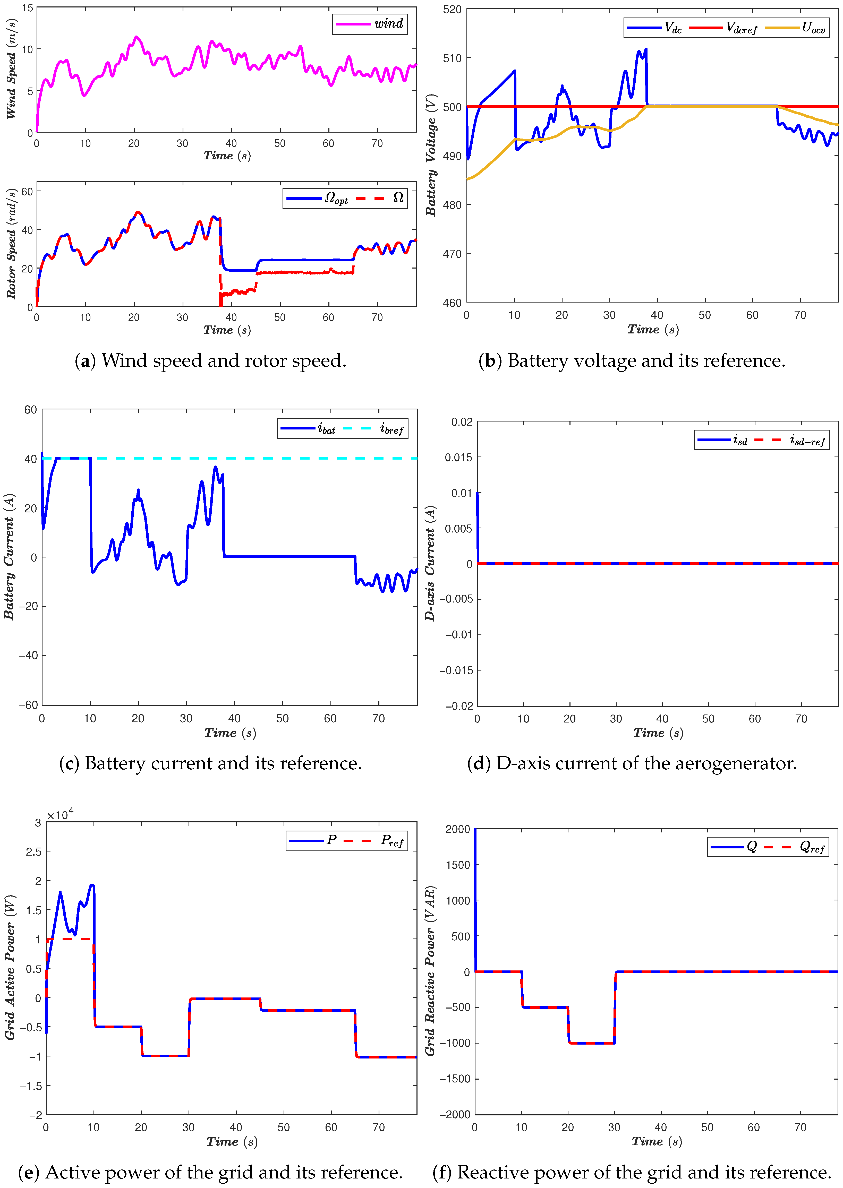
In order to evaluate the performance of the nonlinear controllers defined in Equations (24), (34), (39), (58), (64), (72), and (78), a random wind profile has been considered in this subsection. Figure 5a (top) illustrates the variations in wind speed, ranging from 0 m/s to 15 m/s, over the time interval [0, 78] s. Figure 5a (bottom) shows the evolution of the synchronous generator speed ($\Omega$) along with the optimal reference speed (${\Omega }_{opt}$).

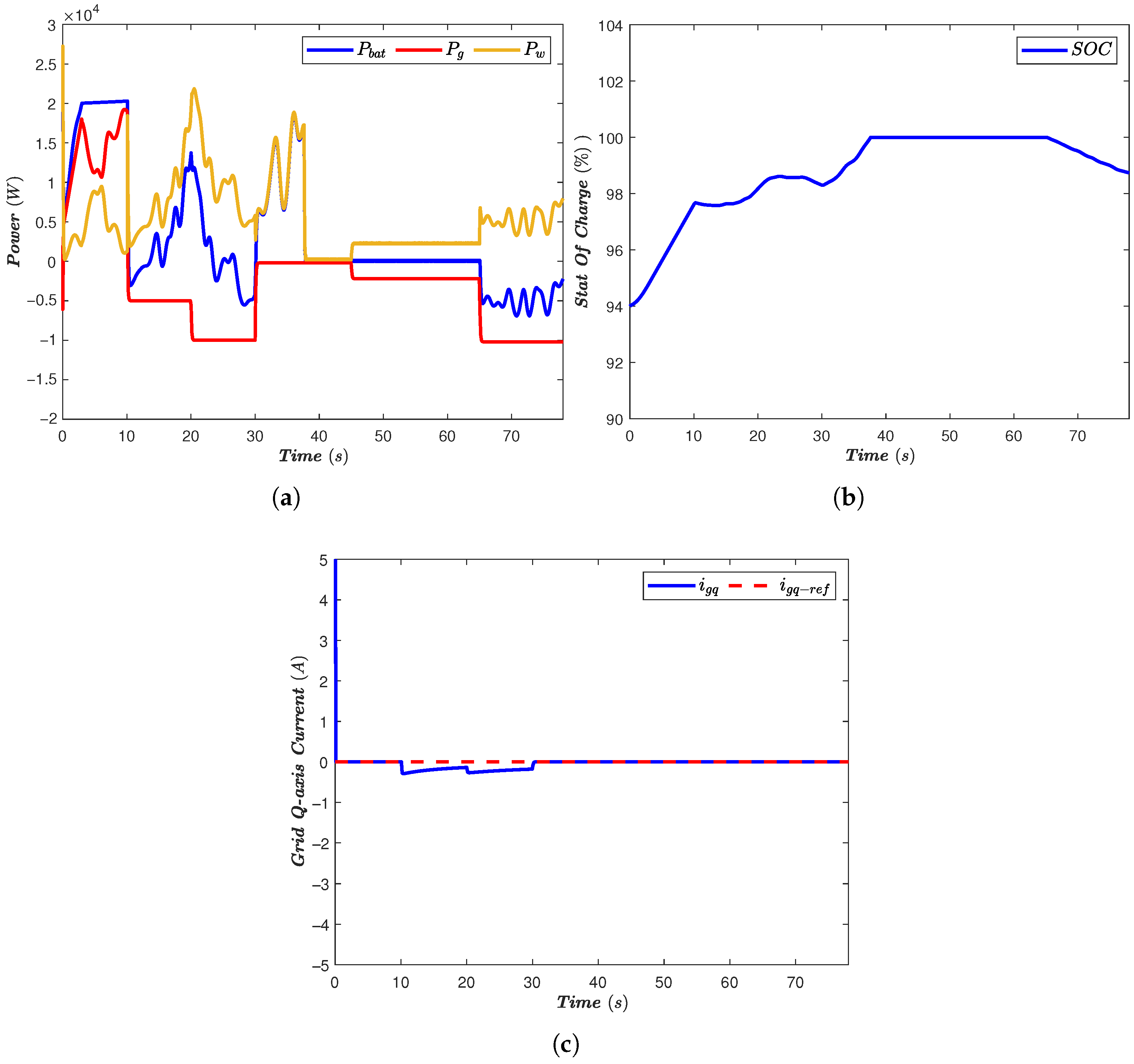
The reference values for the closed-loop current and voltage are set to $i_{b-ref}=40$ A and $v_{b-ref}=500$ V, respectively. Figure 5c,d illustrate the battery’s current and voltage curves, respectively, while the state of charge is presented in Figure 6b.

Throughout the interval [0, 10] s, the battery is not fully charged, the grid is able to supply power, resulting in a current flow. In this phase, the MPPT mode and CC2 mode are active, and it is observed that the synchronous generator speed ($\Omega$) perfectly aligns with the optimal speed ${\Omega }_{opt}$ provided by the optimizer. The battery charges at the maximum current $i_{bat}=i_{b-ref}$.

During the time interval [10, 38] s, the grid demands power, and the algorithm switches to MPPT and power regulation mode. The speed $\Omega$ accurately follows its optimal reference (${\Omega }_{opt}$), and the power regulator forces the active and reactive power to match their respective references $P_{ref}$ and $Q_{ref}$ (Figure 5e,f).

At t = 37 s, the battery becomes fully charged (Figure 6b), and the algorithm switches to constant voltage mode (CV1) maintaining the battery voltage at its maximum value $v_{b-ref}=500V$, and since we have a power balance in the network, the GSC disconnects the battery (OFF).

At t = 44 s, we observe a low power demand from the grid, the MSC remains in MPPT mode, and as long as the power extracted is sufficient to meet the network’s needs, the battery always remains charged and the GSC switches to CV1 mode.

The instant t = 65 s marks a strong demand from the network, the MSC continues in MPPT mode, the GSC switches to power regulation mode (P, Q) and the battery provides the power difference and the SOC decreases.

The performance of the other nonlinear controller for the direct current of the aerogenerator and the grid quadrature current is illustrated in Figure 5d and Figure 6c, where it is observed that $i_{sd}$ is regulated to its reference ($i_{sd-ref}=0$). In parallel with the CC2 mode, the $i_{gq}$ current regulator ensures that it aligns with its reference $i_{gq-ref}=0$.

6.2. The Observer Performances

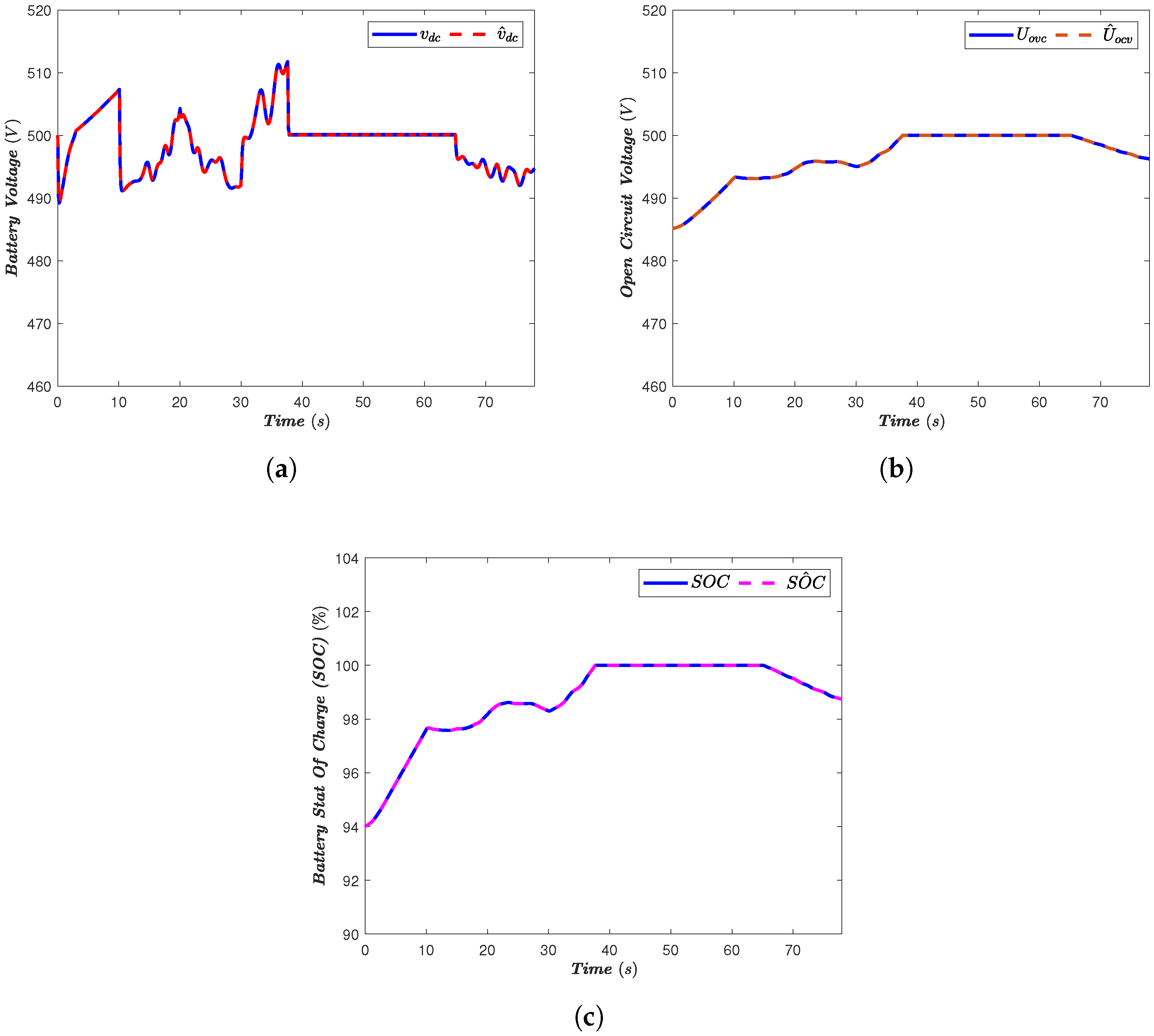
The performance of the proposed observer is demonstrated in Figure 7. In Figure 7a, the battery voltage ($v_{dc}$) is compablack with the observer’s estimated voltage (${\widehat{v}}_{dc}$), showing a perfect match between the two. Figure 7b presents the open-circuit voltage ($U_{ocv}$) alongside its estimated value (${\widehat{U}}_{ocv}$), highlighting the observer’s high estimation accuracy. The battery’s state of charge, calculated using a polynomial P as a function of $U_{ocv}$, is illustrated in Figure 7c. These results strongly confirm the high accuracy and reliability of the proposed observer.

6.3. Quantitative Performance Comparison

For a quantitative performance assessment, the proposed method is compared with a conventional PI controller over the time interval $[10\mathrm{s},38\mathrm{s}]$. The comparison is carried out using the tracking errors associated with the grid active power, the grid reactive power, and the rotor speed, respectively defined as

$$e_1\left(t\right)=P\left(t\right)-P_{ref}\left(t\right),$$

(91)

$$e_2\left(t\right)=Q\left(t\right)-Q_{ref}\left(t\right),$$

(92)

and

$$e_3\left(t\right)=\Omega \left(t\right)-{\Omega }_{opt}\left(t\right).$$

(93)

To evaluate the control performance, two standard integral criteria are considered, namely the Integral Absolute Error (IAE) and the Integral Squared Error (ISE), given by

$$IA{E}_i={\int }_{10}^{38}\left|e_i\left(t\right)\right|dt,i=1,2,3$$

(94)

and

$$IS{E}_i={\int }_{10}^{38}{e}_i^2\left(t\right)dt,i=1,2,3.$$

(95)

These indices make it possible to quantitatively compare the two control approaches in terms of tracking accuracy and overall dynamic performance.

Table 5. Comparative analysis between the PI controller and the proposed method over the time interval $[10\mathrm{s},38\mathrm{s}]$.

	PI Control		Proposed Method
	IAE	ISE	IAE	ISE
$e_1=P-P_{ref}$	0.8421	0.6914	0.3617	0.2486
$e_2=Q-Q_{ref}$	0.7685	0.6243	0.3294	0.2218
$e_3=\Omega -{\Omega }_{\mathrm{opt}}$	0.9158	0.7826	0.4021	0.2874
Mean	0.8421	0.6994	0.3644	0.2526

shows that the proposed method outperforms the conventional PI controller for all considered variables over the interval $[10\mathrm{s},38\mathrm{s}]$. Indeed, both the IAE and ISE values are significantly reduced for the grid active power, grid reactive power, and rotor speed errors when the proposed controller is used. This indicates that the proposed strategy ensures more accurate reference tracking and smaller accumulated deviations than the PI-based approach. The improvement is particularly visible in the rotor speed response, which confirms the better dynamic behavior of the proposed nonlinear controller under operating variations. Overall, these results demonstrate the superior control performance and robustness of the proposed method in comparison with the conventional PI controller.

7. Conclusions

This paper presented a robust solution for integrating wind power into the grid, tackling intermittency and battery management challenges. The system combined a PMSG wind turbine, Vienna rectifiers, and a Li-ion battery, all controlled by a sophisticated adaptive nonlinear control scheme.

Key contributions include:

• A comprehensive model of the entire wind–energy–storage system.
• A suite of sliding mode controllers that ensure stable operation under various conditions, including MPPT, voltage regulation, and precise grid power injection.
• An accurate observer for estimating the battery’s state of charge to protect its health.
• An intelligent energy management algorithm that dynamically coordinates operation based on grid frequency and battery SOC.

Simulation results demonstrated the system’s excellence in maintaining stability, maximizing power extraction, and providing grid support. This work provides a reliable framework for increasing the share of wind energy in modern power systems while ensuring grid stability and prolonging battery life. Future work will focus on experimental validation.

References

1. Hassan, Q.; Viktor, P.; J. Al-Musawi, T.; Mahmood Ali, B.; Algburi, S.; Alzoubi, H.M.; Khudhair Al-Jiboory, A.; Zuhair Sameen, A.; Salman, H.M.; Jaszczur, M. The renewable energy role in the global energy Transformations. Renew. Energy Focus 2024, 48, 100545. [Google Scholar] [CrossRef]
2. Dong, K.; Jiang, Q.; Liu, Y.; Shen, Z.; Vardanyan, M. Is energy aid allocated fairly? A global energy vulnerability perspective. World Dev. 2024, 173, 106409. [Google Scholar] [CrossRef]
3. Mansouri, A.; Ammar, A.; El Magri, A.; Lajouad, R.; Giri, F. Efficiency enhancement through hybrid integration of five-phase PMSG with photovoltaic generator with Vienna rectifier. Sci. Afr. 2024, 26, e02376. [Google Scholar] [CrossRef]
4. Elaadouli, N.; Lajouad, R.; El Magri, A.; Watil, A.; Mansouri, A.; El Myasse, I. An improved control for a stand-alone WEC system involving a Vienna rectifier with battery energy storage management. J. Energy Storage 2024, 76, 109716. [Google Scholar] [CrossRef]
5. Song, T.; Teh, J. Coordinated integration of wind energy in microgrids: A dual strategy approach leveraging dynamic thermal line rating and electric vehicle scheduling. Sustain. Energy Grids Netw. 2024, 38, 101299. [Google Scholar] [CrossRef]
6. Mansouri, A.; El-Bakkouri, J.; El Magri, A.; Elaadouli, N.; El Myasse, I.; Lajouad, R.; Giri, F. Theoretical Development and Experimental Evaluation of a Nonlinear Observer for Sensorless WECS; Elsevier: Amsterdam, The Netherlands, 2024; Volume 58, pp. 1–6. [Google Scholar] [CrossRef]
7. Petersen, C.; Reguant, M.; Segura, L. Measuring the impact of wind power and intermittency. Energy Econ. 2024, 129, 107200. [Google Scholar] [CrossRef]
8. El Khlifi, Y.; El Magri, A.; Mansouri, A.; Lajouad, R.; Chakir, H.E.; Elaadouli, N. Nonlinear Control Design of MFCI for PMSG WECS with Low Voltage Ride-Through Enhancement. Lect. Notes Electr. Eng. 2024, 1141, 519–531. [Google Scholar] [CrossRef]
9. Lajouad, R.; Magri, A.E.; Fadili, A.E.; Chaoui, F.Z.; Giri, F. Adaptive Nonlinear Control of Wind Energy Conversion System Involving Induction Generator. Asian J. Control 2015, 17, 1365–1376. [Google Scholar] [CrossRef]
10. El Magri, A.; Giri, F.; Besançon, G.; El Fadili, A.; Dugard, L.; Chaoui, F. Sensorless adaptive output feedback control of wind energy systems with PMS generators. Control Eng. Pract. 2013, 21, 530–543. [Google Scholar] [CrossRef]
11. Njoka, G.M.; Mogaka, L.; Wangai, A. Impact of variable renewable energy sources on the power system frequency stability and system inertia. Energy Rep. 2024, 12, 4983–4997. [Google Scholar] [CrossRef]
12. Malik, F.H.; Khan, M.W.; Rahman, T.U.; Ehtisham, M.; Faheem, M.; Haider, Z.M.; Lehtonen, M. A Comprehensive Review on Voltage Stability in Wind-Integrated Power Systems. Energies 2024, 17, 644. [Google Scholar] [CrossRef]
13. Mansouri, A.; Elaadouli, N.; Magri, A.E.; Lajouad, R.; Giri, F. Adaptive nonlinear control and observation for grid-connected wind-BESS systems with unknown demand. Unconv. Resour. 2026, 9, 100271. [Google Scholar] [CrossRef]
14. Yang, Z.; Liu, H.; Yuan, Y.; Li, M. Can renewable energy development facilitate China’s sustainable energy transition? Perspective from Energy Trilemma. Energy 2024, 304, 132160. [Google Scholar] [CrossRef]
15. Pan, Y.; Yang, M.Y. Research on the impact of digital infrastructure on the allocation efficiency of green resources in the service industry. Am. J. Econ. Sociol. 2024, 83, 223–247. [Google Scholar] [CrossRef]
16. Alajrash, B.H.; Salem, M.; Swadi, M.; Senjyu, T.; Kamarol, M.; Motahhir, S. A comprehensive review of FACTS devices in modern power systems: Addressing power quality, optimal placement, and stability with renewable energy penetration. Energy Rep. 2024, 11, 5350–5371. [Google Scholar] [CrossRef]
17. El Zoghby, H.M.; Ramadan, H.S. Isolated microgrid stability reinforcement using optimally controlled STATCOM. Sustain. Energy Technol. Assess. 2022, 50, 101883. [Google Scholar] [CrossRef]
18. Khlifi, Y.E.; Magri, A.E.; Mansouri, A.; Lajouad, R. Enhanced low voltage ride-through control of multilevel flying capacitor inverter based wind generation. Indones. J. Electr. Eng. Comput. Sci. 2024, 33, 854–861. [Google Scholar] [CrossRef]
19. Saleem, M.I.; Saha, S.; Roy, T.K.; Ghosh, S.K. Assessment and management of frequency stability in low inertia renewable energy rich power grids. IET Gener. Transm. Distrib. 2024, 18, 1372–1390. [Google Scholar] [CrossRef]
20. Aljarrah, R.; Fawaz, B.B.; Salem, Q.; Karimi, M.; Marzooghi, H.; Azizipanah-Abarghooee, R. Issues and Challenges of Grid-Following Converters Interfacing Renewable Energy Sources in Low Inertia Systems: A Review. IEEE Access 2024, 12, 5534–5561. [Google Scholar] [CrossRef]
21. Singh, P.; Arora, K.; Rathore, U.C.; Joshi, G.P.; Cho, W. Comparative study of controllers in battery energy storage system integrated with doubly fed induction generator-based wind energy conversion system for power quality improvement. Energy Rep. 2024, 11, 4587–4600. [Google Scholar] [CrossRef]
22. Saleem, M.S.; Abas, N. Optimizing renewable polygeneration: A synergetic approach harnessing solar and wind energy systems. Results Eng. 2024, 21, 101743. [Google Scholar] [CrossRef]
23. Akinsooto, O.; Ogundipe, O.B.; Ikemba, S. Regulatory policies for enhancing grid stability through the integration of renewable energy and battery energy storage systems (BESS). Int. J. Frontline Res. Rev 2024, 2, 022–044. [Google Scholar] [CrossRef]
24. Jain, D.; Saxena, D. Comprehensive review on control schemes and stability investigation of hybrid AC-DC microgrid. Electr. Power Syst. Res. 2023, 218, 109182. [Google Scholar] [CrossRef]
25. Yu, C.; Xu, H.; Liu, C.; Chen, C.; Sun, M.; Zhang, X. Research on Modeling, Stability and Dynamic Characteristics of Voltage-controlled Grid-connected Energy Storage Inverters Under High Penetration. Int. J. Electr. Power Energy Syst. 2022, 143, 108397. [Google Scholar] [CrossRef]
26. Jang, Y.; Sun, Z.; Ji, S.; Lee, C.; Jeong, D.; Choung, S.; Bae, S. Grid-Connected Inverter for a PV-Powered Electric Vehicle Charging Station to Enhance the Stability of a Microgrid. Sustainability 2021, 13, 14022. [Google Scholar] [CrossRef]
27. Pelosi, D.; Gallorini, F.; Alessandri, G.; Barelli, L. A Hybrid Energy Storage System Integrated with a Wave Energy Converter: Data-Driven Stochastic Power Management for Output Power Smoothing. Energies 2024, 17, 1167. [Google Scholar] [CrossRef]
28. Martorana, P.; Castellano, A.; Cammalleri, M.; Franzitta, V. Electro-Mechanical WEC Stabilization for Onshore Wave Energy Exploitation. In Proceedings of the OCEANS 2024—Singapore; IEEE: Piscataway, NJ, USA, 2024; pp. 1–6. [Google Scholar] [CrossRef]
29. Xiong, L.; Huang, S.; Li, P.; Wang, Z.; Khan, M.W.; Niu, T. Hidden Markov Jump System Based Robust Control of Inverter-Fed Power Systems With Asynchronous Sliding Mode Observer. IEEE Trans. Ind. Electron. 2025, 72, 13287–13299. [Google Scholar] [CrossRef]
30. Xiong, L.; Li, T.; Huang, S.; Li, P.; Wang, Z.; Sun, Z.; Niu, T. Optimized Sizing of ESSs in Non-Array Formed Wind Farm for Frequency Support Considering Multi-Directional Wake Effect. IEEE Trans. Sustain. Energy 2026, 17, 1878–1893. [Google Scholar] [CrossRef]
31. Elaadouli, N.; Lajouad, R.; El Magri, A.; Mansouri, A.; Elmezdi, K. Efficiency optimization and power flow control in a wind energy conversion system with storage via vienna rectifier. IFAC-PapersOnLine 2024, 58, 454–459. [Google Scholar] [CrossRef]
32. Elaadouli, N.; Lajouad, R.; Magri, A.E.; Mansouri, A.; Elmezdi, K. Adaptive control strategy for energy management in a grid-connected Battery Energy Storage System using a bidirectional Vienna rectifier. J. Energy Storage 2024, 104, 114382. [Google Scholar] [CrossRef]
33. Lu, X.; Xie, Y.; Chen, L. Feedback Linearization and Sliding Mode Control for VIENNA Rectifier Based on Differential Geometry Theory. Math. Probl. Eng. 2015, 2015, 573016. [Google Scholar] [CrossRef]
34. El Mezdi, K.; El Magri, A.; Watil, A.; El Myasse, I.; Bahatti, L.; Lajouad, R.; Ouabi, H. Nonlinear control design and stability analysis of hybrid grid-connected photovoltaic-Battery energy storage system with ANN-MPPT method. J. Energy Storage 2023, 72, 108747. [Google Scholar] [CrossRef]
35. El Myasse, I.; El Magri, A.; Watil, A.; Ashfaq, S.; Kissaoui, M.; Lajouad, R. Improvement of real-time state estimation performance in hvdc systems using an adaptive nonlinear observer. IFAC J. Syst. Control 2024, 27, 100244. [Google Scholar] [CrossRef]
Figure 1. Proposed WECS with grid-connected BESS using Vienna rectifier and bidirectional Vienna rectifier.
Energies 19 01941 g001
Figure 2. (a) The battery open circuit voltage. (b) The battery model and the U o c v .
Energies 19 01941 g002
Figure 3. Flowchart of the proposed energy management strategy.
Energies 19 01941 g003
Figure 4. The proposed control strategy.
Energies 19 01941 g004
Figure 5. Performance of the energy management system with a random wind profile.
Energies 19 01941 g005
Figure 6. Observer performances. (a) Power of the grid, battery, and aerogenerator. (b) State of charge of the battery. (c) Grid quadrature current.
Energies 19 01941 g006
Figure 7. Observer performances. (a) The true Battery Voltage (Blue) and its estimate (red). (b) The Open Circuit Voltage (Blue) and its estimate (orange). (c) The State of Charge (Blue) and its estimate (purple).
Energies 19 01941 g007