Coordinated Optimization of Cross-Line Electric Bus Scheduling and Photovoltaic–Storage–Charging Depot Configuration

Abstract

Amid the global decarbonization of urban transportation, the large-scale deployment of electric buses faces major challenges, including concentrated charging demand, increased peak electricity demand, and inefficient energy utilization at transit depots. Existing studies usually optimize depot energy system configuration and bus scheduling separately, which often leads to biased system-level decisions. To address this limitation, this study proposes a collaborative optimization framework that integrates cross-line scheduling with the configuration of photovoltaic–storage–charging systems at depots to improve overall resource utilization. Specifically, this study formulates a mixed-integer linear programming (MILP) model to minimize the total daily system cost. The proposed model comprehensively captures multiple factors, including the costs of bus investment, charging infrastructure, photovoltaic deployment, energy storage deployment, and carbon emissions. In this study, Benders decomposition is used as a solution framework to handle the coupling structure of the model. Case studies show that, compared with conventional operation modes, the combination of cross-line scheduling and fast charging technology produces a significant synergistic effect. This combination reduces the required fleet size from 17 to 14 buses and substantially lowers investment in depot infrastructure, thereby minimizing the total system cost. Sensitivity analysis further shows that the deployment scale of photovoltaic systems has a clear threshold effect on electricity costs, whereas the core economic value of energy storage systems depends on peak shaving and arbitrage under time-of-use electricity pricing. Overall, this study demonstrates the critical role of integrated planning in improving the economic efficiency and operational feasibility of electric bus systems. It provides important theoretical support and practical guidance for depot design and resource scheduling in low-carbon public transportation networks.

1. Introduction

Climate change mitigation requires deep and sustained emission reductions over the coming decades, making low-carbon transitions in both the energy sector and end-use sectors a common priority [1]. In China, the power system is rapidly moving toward cleaner generation, with wind and solar accounting for most newly installed capacity in recent years [2]. At the same time, road transport remains a major source of energy-related emissions, and electrification is widely viewed as a key pathway for mitigation [3,4]. Among electrified public transport options, battery electric buses are particularly attractive because of their fixed routes, high passenger throughput, and strong per-bus emission reduction potential. Their relatively predictable timetables and centralized depot operations also create favorable conditions for coordinated charging management. By the end of 2024, China had 658,200 public buses and trolleybuses, of which 487,500 were pure electric buses, accounting for 69.4% of the total fleet [5].

Despite these advantages, the large-scale deployment of BEBs introduces new operational and planning challenges for urban distribution networks and depot energy systems. Depot charging is often concentrated and high-power, and the simultaneous charging of multiple buses can therefore create sharp load peaks and increase exposure to demand charges [6]. In addition, charging demand is often temporally misaligned with distributed photovoltaic (PV) generation, which reduces on-site renewable energy utilization and may increase system balancing costs [7]. This situation has driven the transition of traditional charging depots toward integrated energy hubs that combine PV, energy storage, and chargers, and may even provide flexibility value to the power system [8]. A central research question thus emerges: how should a BEB depot be planned and operated to satisfy transport service requirements while jointly minimizing investment cost, electricity cost, and carbon cost?

Existing studies related to BEB depots can be broadly grouped into three streams. The first stream focuses on depot configuration optimization, which typically determines the capacities of PV systems and battery energy storage systems, as well as the number of chargers, under cost minimization or life-cycle objectives. Recent studies no longer treat depot configuration as a stand-alone sizing problem; instead, they increasingly co-optimize charging infrastructure, bus charging schedules, and local PV–storage resources under time-varying energy supply conditions and, in some cases, distribution-network constraints [9,10,11,12], while others improve PV model fidelity through equivalent-circuit modeling and genetic-algorithm-based parameter identification under real outdoor conditions [13]. Charging modes are also differentiated. Comparative analyses suggest that fast charging can increase unit infrastructure cost and sometimes electricity expenditure, but it may also reduce the required fleet size by improving bus turnover, thereby lowering the total system cost under certain conditions [14,15,16]. Engineering details such as conversion efficiency and battery degradation have been incorporated to improve realism and to avoid uneconomic operation patterns [17,18]. However, most configuration studies treat the charging demand profile on the transport side as exogenous. Timetables, bus assignments, and charging windows are often assumed to be fixed, so the configuration solution may not remain optimal when operating organization changes or when the charging strategy shifts.

The second research stream examines bus scheduling and charging operation from the perspectives of transportation science and operations research. Foundational support for this stream is provided by classical bus scheduling models and related review studies [19,20]. Traditional route-based scheduling limits resource sharing across lines and may lead to idle time and bus redundancy when demand differs among routes [21]. To address this limitation, cross-line dispatching has therefore been proposed to improve bus utilization, and recent studies have reported substantial reductions in fleet size, including in electrified bus networks [22,23]. Further extensions consider travel-time variability, passenger-oriented objectives, and tailored solution algorithms [24,25]. For electric buses, scheduling must also account for battery range, charging time windows, and charger availability. This motivates integrated scheduling–charging formulations and efficient algorithms such as branch-and-price or column generation for large-scale instances [26,27,28,29,30,31]. However, these studies mainly focus on operational coordination under given infrastructure conditions. Although charging feasibility is explicitly modeled, depot-side energy-system configuration, such as PV capacity, ESS sizing, and charger planning, is usually not optimized simultaneously with vehicle trip organization. These studies collectively imply that the charging demand profile is not a fixed input but is shaped by dispatching decisions and charging modes.

The third research stream explores joint optimization, as depot investment and bus scheduling are inherently interdependent. As a result, a sequential paradigm may lead to suboptimal decisions. Some studies integrate charger planning and scheduling decisions into unified models and show that joint planning can reduce annualized or life-cycle cost [32]. Under opportunity charging, several studies simultaneously optimize battery size, service frequency, and fleet size to improve economic performance [33,34]. More recently, joint optimization has evolved from coupling charger deployment with bus scheduling to broader transportation–energy coordination frameworks that also incorporate PV, battery storage, grid impacts, carbon objectives, and uncertainty [35]. Nevertheless, in most of these integrated studies, the scheduling layer mainly refers to charging scheduling or charging operation, while vehicle trip organization, bus assignment, and cross-line task chaining remain exogenous or are only simplistically represented. Therefore, cross-line dispatching and depot-side renewable configuration are still seldom modeled simultaneously within one unified optimization framework.

This leaves two practical gaps. First, the economic implications of charging mode selection, fast charging versus slow charging, should be evaluated together with both scheduling and PV–storage sizing, rather than in isolation. Second, cross-line dispatching can reduce fleet size and reshape the time distribution of depot charging demand, which may fundamentally alter the optimal configuration of PV, storage, and chargers, as well as the resulting exposure to demand charges.

To address these gaps, this paper develops a unified optimization framework for bus depots that jointly plans fleet size and task-chain dispatching, charger quantity under fast and slow charging options, and the capacities of PV systems and battery energy storage systems, while accounting for time-of-use pricing, demand charge, and carbon trading cost. Cross-line dispatching is explicitly modeled to enable bus resource sharing across multiple routes. Using the same input data and constraints, four operating scenarios are compared, namely, conventional versus cross-line dispatching and slow versus fast charging, to quantify how operating organization and charging strategy reshape the optimal configuration and cost structure. The results show that cross-line dispatching reduces fleet redundancy and total cost, and that fast charging can further reduce system cost by improving bus turnover even with higher charger unit cost. In addition, PV adoption exhibits a clear threshold effect with respect to levelized PV cost, while energy storage remains valuable mainly for time shifting and peak-related cost mitigation under operational constraints. These findings provide actionable guidance for integrated planning of PV–storage–charging bus depots and for coordinated selection of dispatching and charging strategies.

The main contributions of this study are summarized as follows:

• A unified optimization framework is developed to jointly determine cross-line bus task chaining and depot energy system configuration, thereby coupling bus operations with PV capacity planning, ESS sizing, and charger deployment to coordinate transport service and energy management at the system level.
• A compact MILP formulation is developed to represent cross-line task chaining and heterogeneous charging strategies in an integrated planning setting. The model uses task-level charging variables to capture charging feasibility while avoiding the dimensional expansion caused by trip-pair–time indexed charging decisions.
• A comprehensive cost model is established to capture the economic interactions between fleet operation and depot energy planning. The objective function includes bus and charger investment costs, PV and ESS costs, electricity purchase costs, peak-demand charges, and carbon trading costs, thereby enabling a realistic assessment.
• Scenario-based analyses are conducted across four combinations of scheduling and charging strategies. The results quantify clear synergistic effects: cross-line operation reduces fleet redundancy and the required fleet size, while fast charging improves bus turnover and infrastructure utilization, jointly leading to a notable reduction in total cost.
• Sensitivity analyses on PV and ESS capital costs are performed to identify configuration thresholds. PV adoption exhibits tariff-linked breakpoints, whereas ESS value is mainly driven by time shifting and peak-demand mitigation, providing guidance for planning under evolving technology costs.

2. Proposed Model Description

This section presents the proposed coordinated optimization model for an electric bus depot integrating PV generation, energy storage, and charging facilities. The model jointly considers bus scheduling decisions and depot energy system configuration to minimize the total system cost while satisfying operational and energy constraints.

2.1. System Overview and Problem Description

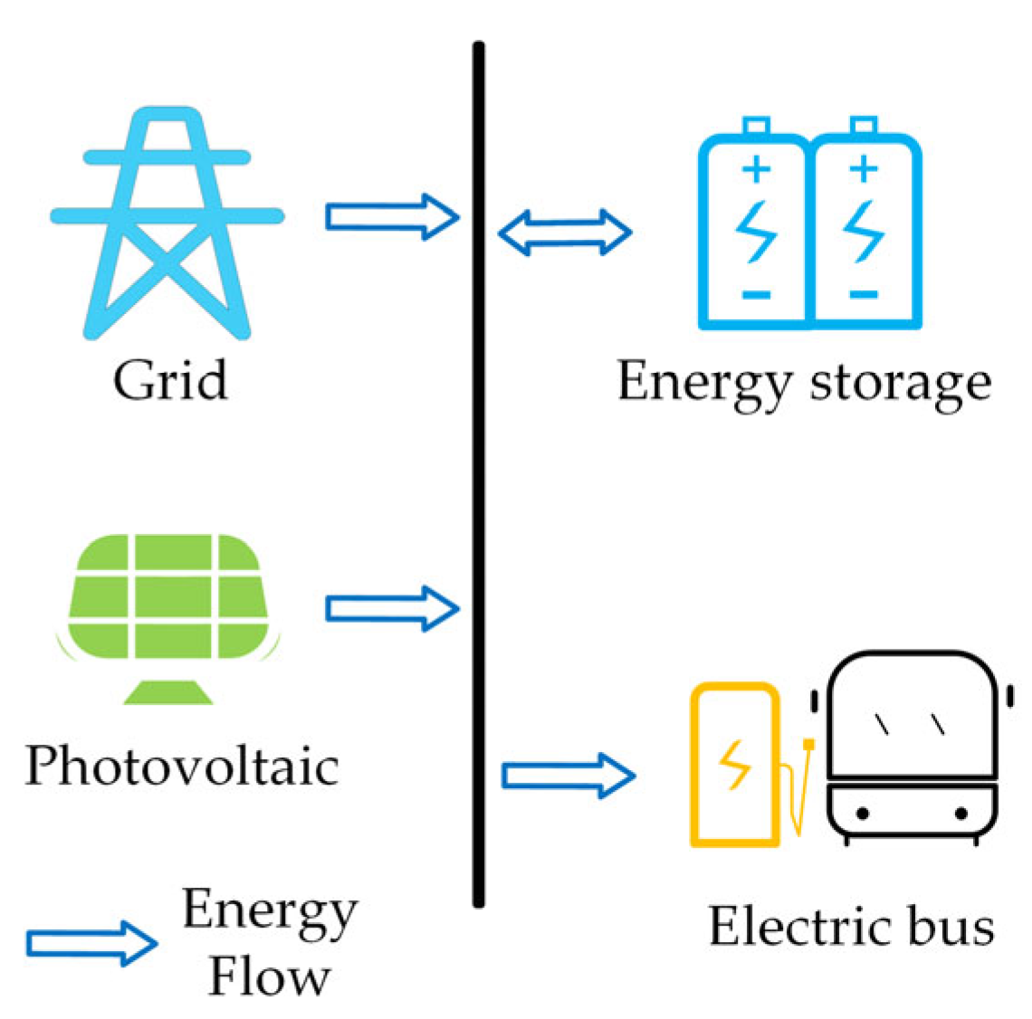
The electric bus depot considered in this study consists of four main components: electric buses, charging infrastructure, a PV system, and an energy storage system. As shown in Figure 1, the depot is connected to the external power grid and can purchase electricity, but does not export power.

From a decision-making perspective, the system involves two tightly coupled subsystems. The bus side subsystem determines bus assignment and scheduling, defining the number of buses required for all scheduled trips and the temporal distribution of charging demand. The depot-side subsystem determines charging infrastructure, PV capacity, and ESS capacity, which affect electricity procurement, peak demand, and renewable energy utilization.

Optimizing bus scheduling and depot configuration separately may lead to mismatches between transport operations and energy system planning. Bus oriented optimization may underestimate infrastructure requirements, whereas depot-oriented optimization may rely on fixed charging patterns that overlook operational flexibility, such as cross-line scheduling and fast charging. Therefore, a unified framework is required to capture the interactions between bus operations and depot energy supply.

This study introduces cross-line scheduling to allow electric buses to operate across multiple routes within a scheduling horizon. Enabling buses to serve successive trips from different routes reduces bus idle time and redundancy. Meanwhile, fast and slow charging modes represent different strategies, affecting charging duration, power demand, and infrastructure utilization.

2.2. Objective Function

The optimization objective is to minimize the daily total system cost, which consists of six components: (1) annualized investment and maintenance costs of electric buses, (2) investment and maintenance costs of charging infrastructure, (3) investment and maintenance costs of the PV system, (4) investment and maintenance costs of the ESS, (5) electricity purchase costs from the grid, including both energy charges and peak demand charges, and (6) carbon emission costs associated with grid electricity consumption. The formulas for the total cost are as follows:

$$\mathrm{m}\mathrm{i}\mathrm{n}\mathrm{C}\mathrm{t}\mathrm{o}\mathrm{t}\mathrm{a}\mathrm{l}=C_{\mathrm{e}\mathrm{b}}+C_{\mathrm{p}\mathrm{v}}+C_{\mathrm{e}\mathrm{s}\mathrm{s}}+C_{\mathrm{c}\mathrm{p}}+C_{\mathrm{g}\mathrm{r}\mathrm{i}\mathrm{d}}+C_{\mathrm{c}\mathrm{a}\mathrm{r}\mathrm{b}\mathrm{o}\mathrm{n}}$$

(1)

The bus-related cost $C_{\mathrm{e}\mathrm{b}}$ accounts for the annualized capital investment and maintenance cost of electric buses. Let $L$ denote the required fleet size, $U_{\mathrm{e}\mathrm{b}}$ the unit purchase cost of an electric bus, and $O_{\mathrm{e}\mathrm{b}}$ the annual maintenance cost per bus. Using a discount rate r and a service life of $y_{\mathrm{e}\mathrm{b}}$ years, the corresponding daily cost is expressed as:

$$C_{\mathrm{e}\mathrm{b}}={\displaystyle \frac{L}{365}}·{\displaystyle \frac{r{(1+r)}^{y_{\mathrm{e}\mathrm{b}}}}{{(1+r)}^{y_{\mathrm{e}\mathrm{b}}}-1}}{U}_{\mathrm{e}\mathrm{b}}+{\displaystyle \frac{L}{365}}·O_{\mathrm{e}\mathrm{b}}$$

(2)

The PV system cost $C_{\mathrm{p}\mathrm{v}}$ consists of the annualized investment cost and operation and maintenance cost of the installed PV capacity. Let $P_{\mathrm{p}\mathrm{v}}^{\mathrm{m}\mathrm{a}\mathrm{x}}$ be the installed PV capacity (kW), $U_{\mathrm{p}\mathrm{v}}$ the unit investment cost, and $O_{\mathrm{p}\mathrm{v}}$ the annual maintenance cost per unit capacity. With a service life of $y_{\mathrm{p}\mathrm{v}}$ years, the daily PV-related cost is:

$$C_{\mathrm{p}\mathrm{v}}={\displaystyle \frac{P_{\mathrm{p}\mathrm{v}}^{\mathrm{m}\mathrm{a}\mathrm{x}}}{365}}·{\displaystyle \frac{r{(1+r)}^{y_{\mathrm{p}\mathrm{v}}}}{{(1+r)}^{y_{\mathrm{p}\mathrm{v}}}-1}}{U}_{pv}+{\displaystyle \frac{P_{\mathrm{p}\mathrm{v}}^{\mathrm{m}\mathrm{a}\mathrm{x}}}{365}}·O_{\mathrm{p}\mathrm{v}}$$

(3)

Similarly, the energy storage system cost $C_{\mathrm{e}\mathrm{s}\mathrm{s}}$ includes the annualized investment and maintenance costs of the ESS. Let $E_{\mathrm{p}\mathrm{v}}^{\mathrm{m}\mathrm{a}\mathrm{x}}$ denote the installed energy capacity of the ESS (kWh), $U_{\mathrm{e}\mathrm{s}\mathrm{s}}$ the unit investment cost, and $O_{\mathrm{e}\mathrm{s}\mathrm{s}}$ the annual maintenance cost per unit capacity. With a service life of $y_{\mathrm{e}\mathrm{s}\mathrm{s}}$ years, the daily ESS cost is given by:

$$C_{\mathrm{e}\mathrm{s}\mathrm{s}}={\displaystyle \frac{E_{\mathrm{e}\mathrm{s}\mathrm{s}}^{\mathrm{m}\mathrm{a}\mathrm{x}}}{365}}·{\displaystyle \frac{r{(1+r)}^{y_{\mathrm{e}\mathrm{s}\mathrm{s}}}}{{(1+r)}^{y_{\mathrm{e}\mathrm{s}\mathrm{s}}}-1}}{U}_{\mathrm{e}\mathrm{s}\mathrm{s}}+{\displaystyle \frac{E_{\mathrm{e}\mathrm{s}\mathrm{s}}^{\mathrm{m}\mathrm{a}\mathrm{x}}}{365}}·O_{\mathrm{e}\mathrm{s}\mathrm{s}}$$

(4)

The charging infrastructure cost $C_{\mathrm{c}\mathrm{p}}$ represents the annualized investment and maintenance cost of the charging piles. Let K be the number of installed charging piles, $U_{\mathrm{c}\mathrm{p}}$ the unit investment cost per charger, and $O_{\mathrm{c}\mathrm{p}}$ the annual maintenance cost. With a service life of $y_{\mathrm{c}\mathrm{p}}$ years, the daily charging infrastructure cost is expressed as:

$$C_{\mathrm{c}\mathrm{p}}={\displaystyle \frac{K}{365}}·{\displaystyle \frac{r{(1+r)}^{y_{\mathrm{c}\mathrm{p}}}}{{(1+r)}^{y_{\mathrm{c}\mathrm{p}}}-1}}{U}_{\mathrm{c}\mathrm{p}}+{\displaystyle \frac{K}{365}}·O_{\mathrm{c}\mathrm{p}}$$

(5)

The electricity purchase cost $C_{\mathrm{g}\mathrm{r}\mathrm{i}\mathrm{d}}$ includes both the energy charge and the peak demand charge. The operation horizon is discretized into a set of time slots $t\in \mathrm{T}$, each with a duration of $∆t$ hours. Let $p_t^{\mathrm{g}\mathrm{r}\mathrm{i}\mathrm{d}}$ denote the grid electricity purchase power (kW) at time slot $t$, and $U_t^{\mathrm{g}\mathrm{r}\mathrm{i}\mathrm{d}}$ the corresponding time-of-use electricity price (CNY/kWh). The purchased energy is given by $E_t^{\mathrm{g}\mathrm{r}\mathrm{i}\mathrm{d}}=p_t^{\mathrm{g}\mathrm{r}\mathrm{i}\mathrm{d}}∆t$. An auxiliary variable $P_{\mathrm{p}\mathrm{e}\mathrm{a}\mathrm{k}}^{\mathrm{g}\mathrm{r}\mathrm{i}\mathrm{d}}$ is introduced to represent the maximum grid purchase power over the day, and $U_{\mathrm{d}\mathrm{e}\mathrm{m}}$ denotes the demand charge rate. The grid electricity cost is calculated as:

$$C_{\mathrm{g}\mathrm{r}\mathrm{i}\mathrm{d}}=\sum _{t\in \mathrm{T}}{E}_t^{\mathrm{g}\mathrm{r}\mathrm{i}\mathrm{d}}{U}_t^{\mathrm{g}\mathrm{r}\mathrm{i}\mathrm{d}}+P_{\mathrm{p}\mathrm{e}\mathrm{a}\mathrm{k}}^{\mathrm{g}\mathrm{r}\mathrm{i}\mathrm{d}}{U}_{\mathrm{d}\mathrm{e}\mathrm{m}}$$

(6)

Finally, the carbon trading cost $C_{\mathrm{c}\mathrm{a}\mathrm{r}\mathrm{b}\mathrm{o}\mathrm{n}}$ is associated with carbon emissions from grid electricity consumption. Let α be the grid emission factor (kg/kWh), $R_{base}$ denotes the carbon emission baseline, which is defined as the carbon emissions of a fuel bus traveling the same distance (kg), and $U_{\mathrm{c}\mathrm{a}\mathrm{r}\mathrm{b}\mathrm{o}\mathrm{n}}$ is the carbon trading price (CNY/kg). The carbon trading quantity is defined as the difference between the actual carbon emissions caused by electricity purchase and the carbon emission baseline. If this value is greater than zero, the depot must purchase additional carbon allowances; if it is less than zero, the depot can sell the surplus allowances, resulting in carbon trading revenue. The carbon cost is expressed as:

$$C_{carbon}=(\sum _{t\in \mathrm{T}}\mathsf{\alpha }{E}_t^{\mathrm{g}\mathrm{r}\mathrm{i}\mathrm{d}}-R_{base})U_{\mathrm{c}\mathrm{a}\mathrm{r}\mathrm{b}\mathrm{o}\mathrm{n}}$$

(7)

2.3. Model Constraints

This section formulates the interlining scheduling problem as assigning all trip tasks to buses while satisfying operational constraints. A bus oriented modeling perspective requires characterizing task transfer relationships for each bus. However, interlining increases potential transfer combinations, leading to excessive decision variables. To address this, tasks executed by each bus are represented as ordered trip chains defining sequential relationships between adjacent tasks. Consequently, all trip tasks are organized into several non-overlapping sequences where each task belongs to exactly one chain corresponding to a single bus.

2.3.1. Trip Connection Constraints

The following constraints ensure that bus trips can be connected into feasible operating chains.

$$(e_i-s_j)x_{ij}\le 0$$

(8)

$$x_{0j}+\sum _{i\in \mathrm{N}}{x}_{ij}=1$$

(9)

$$x_{i,N+1}+\sum _{j\in \mathrm{N}}{x}_{ij}=1$$

(10)

$$L=\sum _{j\in \mathrm{N}}{x}_{0j}$$

(11)

where N denotes the set of all trips; 0 and N + 1 represent the virtual source and sink; $x_{ij}$ is a binary variable indicating whether trip j is served immediately after trip i; $s_i$ and $s_j$ denote the start and end time slots of trip i; and L is the required number of electric buses.

Equation (8) ensures a bus can serve trip j after trip i only if the end time of trip i does not exceed the start time of trip j. Equations (9) and (10) require each trip to have exactly one predecessor and one successor, forming continuous operating chains from a virtual source to a virtual sink. Equation (11) defines the fleet size as the number of trip chains initiated from the virtual source.

2.3.2. Bus Charging Power Constraints

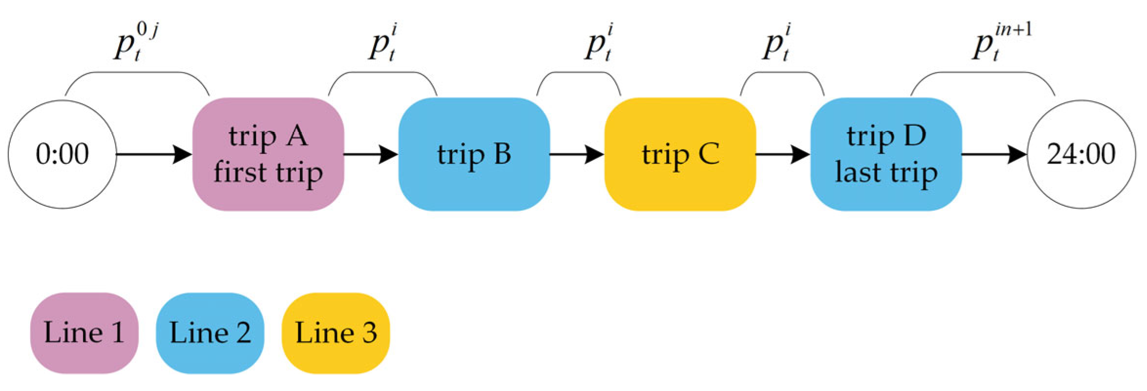
In this study, buses are allowed to charge whenever they are parked at the depot during an available charging window, including not only overnight parking periods but also inter-trip layovers during daytime operation. The following constraints govern bus charging behavior and charging infrastructure capacity. Rather than tracking individual buses, the model defines charging power at the task-time level through $p_t^i$. Since charging is only allowed during idle periods between consecutive tasks, and feasible task chaining and temporal precedence are enforced by the dispatching constraints, $p_t^i$ is sufficient to represent charging allocation during available charging windows. This treatment avoids unnecessary dimensional expansion and keeps the integrated model tractable. Therefore, charging is restricted to the idle intervals between adjacent tasks, as well as the idle time before the first task and after the final task, as illustrated in Figure 2.

$$\left\{\begin{array}{c}0\le p_t^i\le P_{eb}^{max}\\ p_t^i=0\end{array}\right.{\displaystyle \genfrac{}{}{0pt}{}{,t\in [e_i,\sum _{j\in N}{s}_j{x}_{ij}]}{,t\notin [e_i,\sum _{j\in N}{s}_j{x}_{ij}]}}$$

(12)

$$0\le p_t^{0j}\le P_{eb}^{max}{\tau }_t^{0j}·x_{0j}$$

(13)

$$0\le p_t^{i,N+1}\le P_{eb}^{max}{\tau }_t^{i,N+1}·x_{i,N+1}$$

(14)

$$\sum _{i\in \mathrm{N}}(p_t^i+p_t^{0j}+p_t^{i,N+1})\le K{P}_{cp}^{max}$$

(15)

where $p_t^i$ denotes the charging power (kW) of the bus associated with trip i at time slot t, when the bus is idle and available for charging during the scheduling horizon; $p_t^{0j}$ denotes the charging power (kW) at time slot t for a bus whose first assigned trip of the day is trip j. This variable captures the charging behavior during the idle period before the execution of the first trip; $p_t^{i,N+1}$ denotes the charging power (kW) at time slot t for a bus whose last assigned trip of the day is trip i. This variable represents charging during the idle period after completing the final trip; $P_{eb}^{max}$ is the maximum charging power of a bus; ${\tau }_t^{0j}$ is a binary indicator that equals 1 if a bus whose first assigned trip is j is available for charging at time slot t; otherwise, it equals 0. This variable is used to activate charging power variables only during feasible idle periods; ${\tau }_t^{i,N+1}$ indicates whether a bus whose last assigned trip is i is available for charging at time slot t.

Equation (12) associates charging opportunities with the idle intervals between adjacent tasks, while Equation (13) maps these opportunities to the idle periods preceding the first task. Similarly, Equation (14) identifies charging opportunities during the idle time following the final task. Equation (15) restricts the aggregate charging power of all buses during each time period based on the total installed capacity of the charging piles.

2.3.3. Battery Energy Constraints for Buses

The energy feasibility of bus operations is ensured by the following constraints:

$$Q_j=E_{eb}^{ini}{x}_{0j}+\sum _{t\in T}{p}_t^{0j}∆t+\sum _{i\in N}{x}_{ij}(Q_i-h_i+\sum _{t\in T}{p}_t^i∆t)$$

(16)

$$E_{eb}^{min}\le Q_j\le E_{eb}^{max}$$

(17)

where $Q_i$ is the battery energy at the beginning of trip i; $h_i$ is the energy consumption of trip i; $E_{eb}^{min}$ and $E_{eb}^{max}$ are the minimum and maximum allowable battery energy; $E_{eb}^{ini}$ is the initial battery energy at the beginning of the day. Equation (16) describes the energy transition between consecutive trips, accounting for trip energy consumption and charging during idle periods. Equation (17) ensures that the battery energy at the beginning of each trip lies within allowable limits.

In addition, this paper constrains the battery to maintain the same state of charge at the start and end time slots of intraday scheduling, thereby ensuring the comparability and feasibility of the intraday scheduling results:

$$Q_i^{\mathrm{e}\mathrm{n}\mathrm{d}}=E_{eb}^{ini}{x}_{0j}+\sum _{t\in T}{p}_t^{i,N+1}∆t+x_{i,N+1}(Q_i-h_i)$$

(18)

$$Q_i^{\mathrm{e}\mathrm{n}\mathrm{d}}=E_{eb}^{ini}{x}_{i,N+1}$$

(19)

where $Q_i^{\mathrm{e}\mathrm{n}\mathrm{d}}$ is the battery energy at the end of the day when task i is the last task. Equation (18) is used to calculate $Q_i^{\mathrm{e}\mathrm{n}\mathrm{d}}$, and Equation (19) enforces daily cycling of the bus by requiring the final energy level to equal the initial value.

2.3.4. Energy Storage System Constraints

The relationship between the charging and discharging power and energy of the energy storage system should satisfy the following constraints:

$$-P_{ess}^{max}\le p_t^{ess}\le P_{ess}^{max}$$

(20)

$$E_{ess}^{min}\le E_t^{ess}\le E_{ess}^{max}$$

(21)

$$E_t^{ess}=E_{t-1}^{ess}+p_t^{ess}∆t$$

(22)

$$E_T^{ess}=E_{ess}^{ini}$$

(23)

where $p_t^{ess}$ is the ESS power; $E_t^{ess}$ is the stored energy; $P_{ess}^{max}$ is the ESS power limit; $E_{ess}^{min}$ and $E_{ess}^{max}$ are the minimum and maximum allowable battery energy; $E_{ess}^{ini}$ is the initial battery energy at the beginning of the day. Equations (20)–(22) limit the charging and discharging power of the ESS, bound its stored energy, and describe its inter-temporal energy balance. Equation (23) enforces daily cycling of the ESS by requiring the final energy level to equal the initial value.

2.3.5. PV and Power Balance Constraints

PV are only allowed to be installed within the area of the charging station, and the installation area shall not exceed 80% of the total area of the charging station:

$$\delta P_{\mathrm{p}\mathrm{v}}^{\mathrm{m}\mathrm{a}\mathrm{x}}\le {0.8S}^{max}$$

(24)

where $\delta$ is the PV area requirement per unit capacity; $S^{max}$ is the available area; Equation (24) limits the installed PV capacity according to the available installation area.

$$p_t^{\mathrm{g}\mathrm{r}\mathrm{i}\mathrm{d}}+p_t^{\mathrm{p}\mathrm{v}}-p_t^{\mathrm{e}\mathrm{s}\mathrm{s}}=\sum _{i\in \mathrm{N}}(p_t^i+p_t^{0j}+p_t^{i,N+1})$$

(25)

$$P_{\mathrm{p}\mathrm{e}\mathrm{a}\mathrm{k}}^{\mathrm{g}\mathrm{r}\mathrm{i}\mathrm{d}}\ge p_t^{\mathrm{g}\mathrm{r}\mathrm{i}\mathrm{d}}$$

(26)

where $p_t^{\mathrm{p}\mathrm{v}}$ is the PV output power. Equation (25) enforces the power balance at each time slot, ensuring that total charging demand is met by grid electricity, PV generation, and ESS discharging. Equation (26) defines the peak grid power used to calculate the demand charge.

2.3.6. Linearization

Several constraints involve products of binary and continuous variables. To preserve the MILP structure, these nonlinear expressions are reformulated using standard big-M linearization with auxiliary variables.

$$\sum _{t\in T}{b}_{it}=\sum _{j\in N}{s}_j{x}_{ij}$$

(27)

$$b_{it+1}\le b_{it}$$

(28)

$$\left\{\begin{array}{cc}0\le p_t^i\le b_{it}{P}_{eb}^{max}& ,t<e_i\\ p_t^i=0& ,t\ge e_i\end{array}\right.$$

(29)

$$Q_j=E_{\mathrm{e}\mathrm{b}}^{\mathrm{i}\mathrm{n}\mathrm{i}}{x}_{0j}+\sum _{t\in T}{p}_t^{0j}∆t+\sum _{i\in N}{u}_{ij}$$

(30)

$$u_{ij}\le Q_i-h_i+\sum _{t\in T}{p}_t^i∆t+M(1-x_{ij})$$

(31)

$$u_{ij}\ge Q_i-h_i+\sum _{t\in T}{p}_t^i∆t-M(1-x_{ij})$$

(32)

$$0\le u_{ij}\le M{x}_{ij}$$

(33)

$$Q_i^{\mathrm{e}\mathrm{n}\mathrm{d}}=E_{\mathrm{e}\mathrm{b}}^{\mathrm{i}\mathrm{n}\mathrm{i}}{x}_{0j}+\sum _{t\in T}{p}_t^{i,N+1}∆t+u_i^{\mathrm{e}\mathrm{n}\mathrm{d}}$$

(34)

$$u_i^{\mathrm{e}\mathrm{n}\mathrm{d}}\le Q_i-h_i+M\left({1-x}_{i,N+1}\right)$$

(35)

$$u_i^{\mathrm{e}\mathrm{n}\mathrm{d}}\ge Q_i-h_i-M\left({1-x}_{i,N+1}\right)$$

(36)

$$0\le u_i^{\mathrm{e}\mathrm{n}\mathrm{d}}\le M{x}_{i,N+1}$$

(37)

where $b_{it}$, $u_{ij}$, $u_i^{\mathrm{e}\mathrm{n}\mathrm{d}}$ and M are auxiliary variables introduced. Equations (27)–(29) provide the linearized equivalent of Equation (12); Equations (30)–(33) correspond to the linearization of Equation (16); and Equations (34)–(37) are derived to linearize Equation (18). These reformulations ensure that the original logical implications are exactly enforced while maintaining linearity, enabling efficient solution by commercial MILP solvers.

2.3.7. Solution Algorithm Based on Benders Decomposition

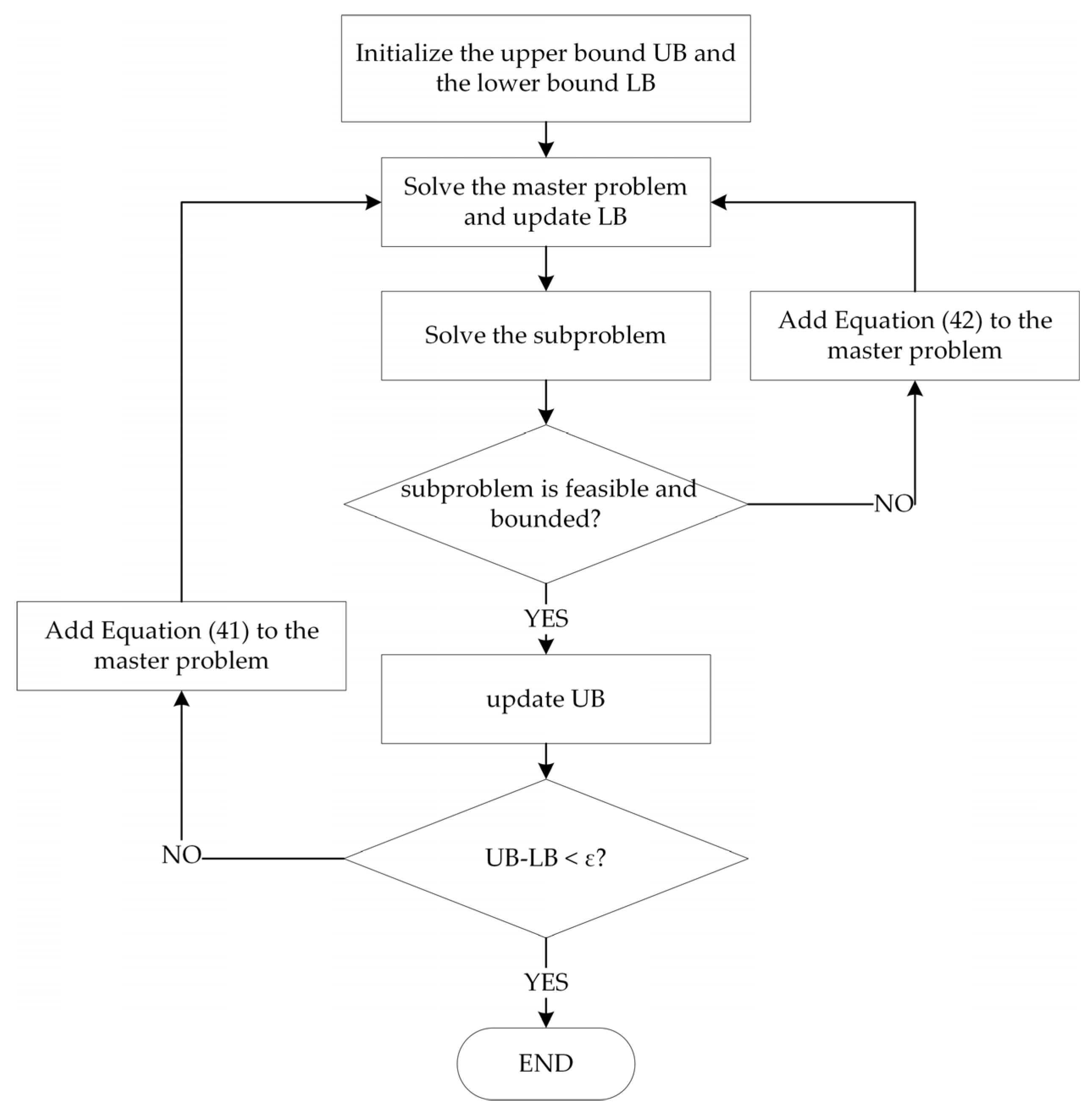
The Benders decomposition algorithm serves as an effective method for solving large-scale MILP models. As established in the preceding sections, the proposed model is a MILP formulation that presents significant computational challenges when applied to large-scale instances. Consequently, this study employs the Benders decomposition algorithm to decouple the configuration optimization model into a master problem and subproblems, which are subsequently resolved through an iterative solution process.

The proposed configuration optimization model incorporates binary variables for bus task assignment and integer variables for the number of charging piles, both of which are classified as hard variables. When these variables are fixed, the remaining subproblem transforms into the minimization of PV and energy storage configuration costs, charging costs, and carbon emission costs based on a predetermined bus operation schedule, as expressed in Equation (38).

$$\begin{gathered} \mathrm{m}\mathrm{i}\mathrm{n}{C}_{\mathrm{p}\mathrm{v}}+C_{\mathrm{e}\mathrm{s}\mathrm{s}}+C_{\mathrm{g}\mathrm{r}\mathrm{i}\mathrm{d}}+C_{\mathrm{c}\mathrm{a}\mathrm{r}\mathrm{b}\mathrm{o}\mathrm{n}} \\ s.t.\left(12\right)-\left(37\right) \end{gathered}$$

(38)

The compact matrix expression is given in Equation (39).

$$\begin{gathered} min{\mathbf{d}}^{\mathrm{T}}\mathbf{y} \\ s.t.\mathbf{T}\mathbf{y}\ge \mathbf{h}-\mathbf{W}\widehat{\mathbf{z}} \end{gathered}$$

(39)

where $\mathbf{y}=[p_t^i,p_t^{0j},p_t^{i,N+1},p_t^{ess},p_t^{\mathrm{g}\mathrm{r}\mathrm{i}\mathrm{d}},Q_j,Q_i^{\mathrm{e}\mathrm{n}\mathrm{d}},E_t^{ess},P_{\mathrm{p}\mathrm{v}}^{\mathrm{m}\mathrm{a}\mathrm{x}},E_{ess}^{max}]$, is variable of the subproblem. $\mathbf{z}=[x_{0j},x_{i,N+1},x_{ij},K]$, is variable of the master problem., $\widehat{\mathbf{z}}$ represents the fixed master problem variable, while d denotes the vector of objective coefficients. The terms T, h, and W are the coefficient matrices of the constraints. Let $\mathsf{\pi }$ be the dual variables associated with the constraints. The dual subproblem is expressed as Equation (40). When the dual subproblem yields a bounded feasible solution, an extreme point ${\mathsf{\pi }}_{*}$ is obtained. Conversely, if the dual subproblem is unbounded, it generates an extreme ray ${\mathsf{\pi }}_{\mathit{\omega }}$.

$$\begin{gathered} \mathrm{m}\mathrm{a}\mathrm{x}{\mathsf{\pi }}^{\mathrm{T}}(\mathbf{h}-\mathbf{W}\widehat{\mathbf{z}}) \\ s.t.{\mathbf{T}}^{\mathrm{T}}\mathsf{\pi }\le \mathbf{d} \end{gathered}$$

(40)

The master problem is transformed into an optimization problem that minimizes the costs associated with buses and charging piles, where $\theta$ is introduced as a lower bound approximation of the optimal cost of the subproblem, formulated as:

$$\begin{gathered} \mathrm{m}\mathrm{i}\mathrm{n}{C}_{\mathrm{e}\mathrm{b}}+C_{\mathrm{c}\mathrm{p}}+\theta \\ s.t.\left(8\right)-\left(11\right)\left(15\right) \end{gathered}$$

(41)

$$\theta \ge {{\mathsf{\pi }}_{*}}^{\mathrm{T}}(\mathbf{h}-\mathbf{W}\mathbf{z})$$

(42)

$$0\ge {{\mathsf{\pi }}_{\mathit{\omega }}}^{\mathrm{T}}(\mathbf{h}-\mathbf{W}\mathbf{z})$$

(43)

where Equation (42) defines the optimality cut constraints, Equation (43) specifies the feasibility cut constraints.

In this study, the iterative process terminates when the gap between the upper and lower bounds satisfies the convergence tolerance $\epsilon$. Upon satisfaction of either condition, the algorithm outputs the optimal feasible solution identified throughout the iterative procedure. The detailed implementation logic is illustrated in Figure 3.

3. Results

This section presents and discusses the numerical results of the proposed coordinated optimization model. The analysis focuses on how different scheduling and charging strategies affect fleet size, infrastructure configuration, energy management behavior, and overall system cost. Four representative scenarios are constructed by combining conventional or cross-line scheduling with slow or fast charging strategies, enabling a systematic comparison of their operational and economic performance.

The proposed model is implemented on a Python 3.12-based platform, and the Benders decomposition procedure is solved using Gurobi 12.0.1. The termination criterion of the decomposition algorithm is a minimum optimality gap of 0.001%. All numerical experiments are conducted on a desktop computer equipped with an Intel Core i9-13900K processor and 32 GB RAM. These settings are reported to improve the transparency of the solution process.

3.1. Experimental Setup and Scenario Description

The case study is conducted based on a real-world electric bus depot serving multiple urban routes. All trips and energy variables are discretized over a unified 24 h horizon with a 15 min time slot to ensure consistent coupling between bus scheduling and the depot energy management problem. Taking a bus depot in Shanghai as a case study,

Table 1. Bus route operation data.

Route	Operating Hours	Headway	Avg. Trip Duration	Avg. Trip Energy
Route 1	6:00–23:00	15 min	44 min	24 kWh
Route 2	6:30–22:30	15 min	60 min	34 kWh
Route 3	6:30–22:00	30 min	58 min	33 kWh
Route 4	6:15–22:00	30 min	105 min	57 kWh

summarizes the daily operating schedules of all routes, including operating hours, departure headways, average one-way trip duration, and average energy consumption.

The key techno-economic parameters of buses, chargers, the PV system, and the energy storage system are listed in

Table 2. Techno-economic parameters of depot equipment.

Item	Unit Price	Lifetime	O&M Cost	Max Power
Electric bus	0.85 million CNY/unit	13 years	1000 CNY/year	350 kW
Fast charger	0.22 million CNY/unit	20 years	1500 CNY/year	350 kW
Slow charger	0.096 million CNY/unit	20 years	1000 CNY/year	120 kW
PV system	2900 CNY/kW	20 years	46 CNY/(kW·year)	-
ESS	640 CNY/kWh	20 years	15 CNY/(kW·year)	300 kW

[36,37].

The time-of-use electricity tariff in Shanghai and the demand charge based on maximum demand are presented in

Table 3. Time-of-use tariff and demand charge.

Period	Time Window	Energy Price (CNY/kWh)
Peak	8–11, 13–15, 18–21	0.916
Flat	6–8, 11–13, 15–18, 21–22	0.567
Valley	22–6 (next day)	0.213
Demand charge	-	1.134

.

In addition, the electric bus has a battery capacity of 200 kWh, the discount rate is 3.5%, the carbon price is set to 0.06 CNY/kg and the average grid carbon emission factor is 0.5834 kg/kWh [38]. The maximum available depot area is 5000 m², and the PV area coefficient is 7.14 m²/kW [39]. These settings are used consistently across all compared scenarios to ensure a fair evaluation of different operating and charging strategies. The PV installation area is limited to 50–80% of the total depot area. The battery starts with zero initial energy. To facilitate model formulation and numerical solution, the following assumptions are adopted:

• The daily bus operation schedule is deterministic and known in advance. Trip departure times, durations, and energy consumption are fixed;
• All electric buses start the day with the same initial state of charge, and the end-of-day state of charge is constrained to return to this initial level;
• Charging and discharging efficiencies of buses and the energy storage system are assumed to be constant;
• The current cost model is based on daily-equivalent cost allocation under assumed service lifetimes and does not explicitly consider bus battery degradation caused by different charging rates or cycling behaviors;
• The PV generation profile is treated as known and deterministic, and reverse power flow to the grid is not allowed.

3.2. Results and Discussion

The evaluation framework consists of four scenarios defined by the integration of bus scheduling strategies and charging infrastructure. Scenario 1 represents non-interlining scheduling where the depot is equipped with slow charging piles, while Scenario 2 utilizes fast charging piles under the same scheduling approach. Scenarios 3 and 4 transition to interlining scheduling, employing slow and fast charging piles respectively to assess the impact of operational flexibility and charging power on system efficiency.

3.2.1. Configuration and Cost Evaluation Across Diverse Scenarios

The specific configurations and costs of each scenario are summarized in

Table 4. Charging station configurations for different scenarios.

Category	Scenario 1	Scenario 2	Scenario 3	Scenario 4
Electric buses (unit)	17	16	16	14
Charging piles (unit)	4	2	4	1
PV system (kW)	560	560	560	560
ESS (kWh)	1543	1700	1700	1800
Carbon (kg)	2740.5	2740.5	2740.5	2740.5
Electricity (kWh)	4364.13	4364.13	4364.13	4364.13
Demand charge (kW)	709.98	709.98	709.98	650

and

Table 5. Daily Comprehensive Cost in Different Scenarios (CNY).

Category	Scenario 1	Scenario 2	Scenario 3	Scenario 4
Electric buses	3888.47	3659.47	3659.47	3202.27
Charging piles	84.82	92.92	84.82	46.45
PV system	362.17	362.17	362.17	362.17
ESS	253.82	279.64	279.64	295.95
Carbon trading	−164.43	−164.43	−164.43	−164.43
Electricity cost	929.56	929.56	929.56	1056.1
Demand charge	805.11	805.11	805.11	737

. In terms of daily total cost, Scenario 4 achieves the lowest value at RMB 5535.32, whereas Scenario 1 has the highest cost at RMB 6159.53. The primary source of cost reduction arises from the bus side. Cross-line scheduling improves task continuity across routes and reduces idle time, thereby lowering fleet redundancy. This effect becomes more pronounced when combined with fast charging, because shorter charging interruptions make it easier for buses to serve denser task chains. As a result, Scenario 4 requires the fewest buses.

Fast charging also significantly reduces charger demand. Its value lies not only in delivering higher charging power, but also in shortening charger occupation time and improving charger turnover. When combined with cross-line scheduling, charging resources can satisfy the same transport demand with far fewer chargers. PV capacity remains unchanged across all scenarios, indicating that under the current tariff, carbon cost, and depot-area settings, PV is consistently economical and insensitive to differences in scheduling strategy. By contrast, ESS capacity increases in Scenario 4. This suggests that when fleet redundancy is reduced, greater flexibility must be provided by depot-side storage to support energy shifting and peak regulation.

Although Scenario 4 incurs slightly higher electricity and storage costs, these increases are offset by much larger reductions in bus cost, charger cost, and demand charges. Therefore, the superiority of Scenario 4 arises from system-wide coordination rather than from minimizing any single cost component.

3.2.2. Analysis of Task Scheduling Across Diverse Scenarios

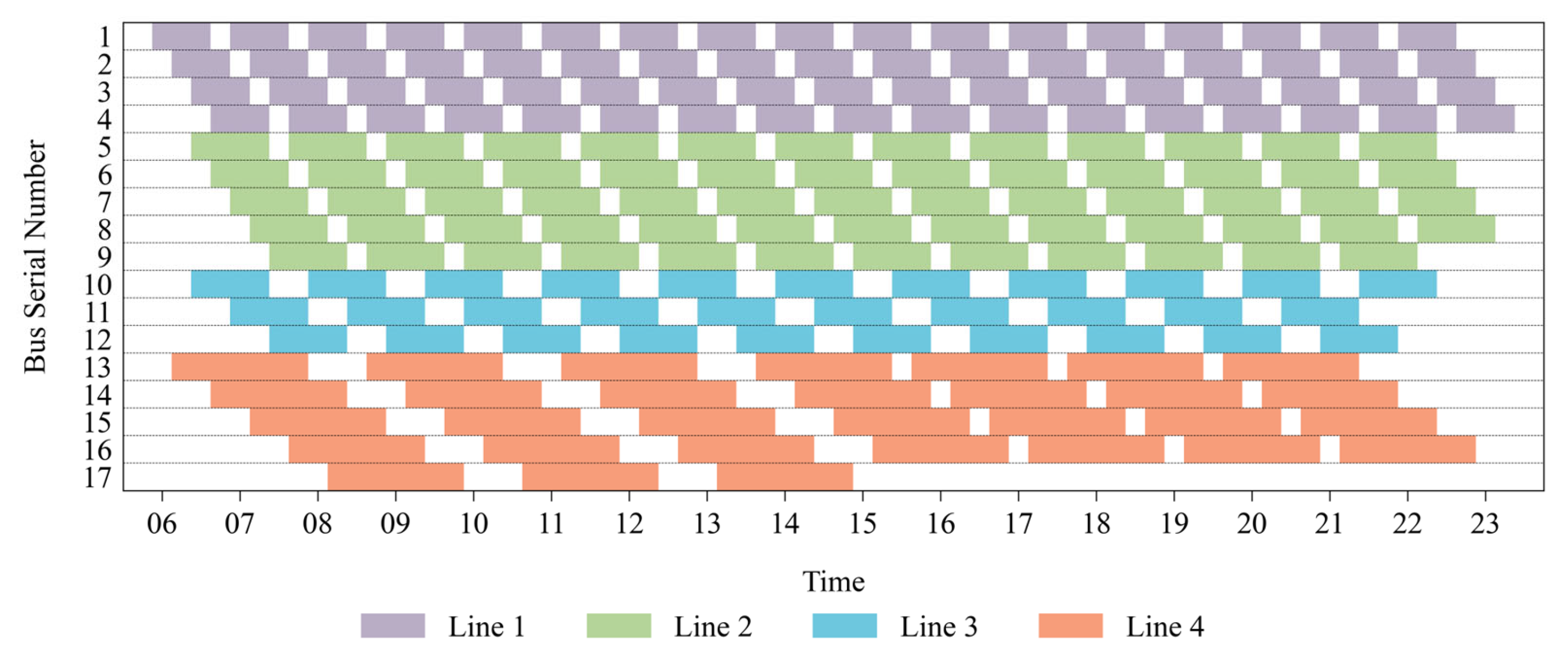
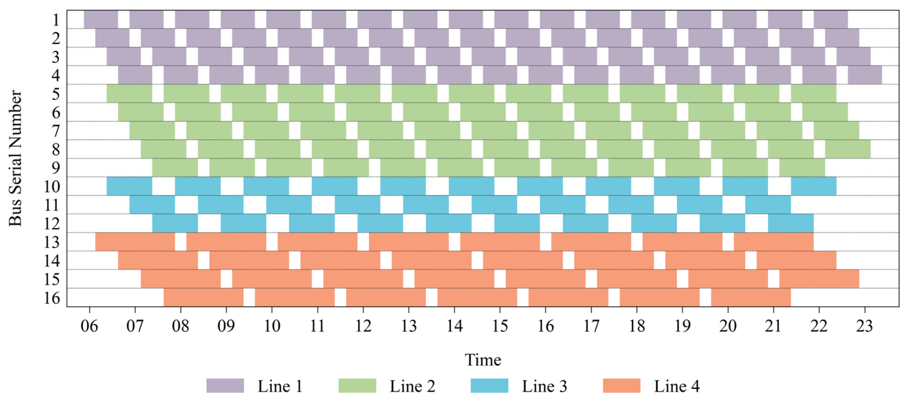
The scheduling pattern in Figure 4 reflects the structural inefficiency of route-fixed operation under slow charging. Because each bus is confined to a single route, idle periods created by headway differences and uneven trip durations cannot be shared across routes. This is particularly evident for Route 4, which has the longest average trip duration and the highest energy consumption among all routes. Under slow charging, buses assigned to this route require longer recovery and charging windows, so additional standby vehicles are needed to preserve timetable feasibility. In contrast, shorter routes exhibit fragmented idle intervals that remain underutilized because they cannot be transferred to support other lines.

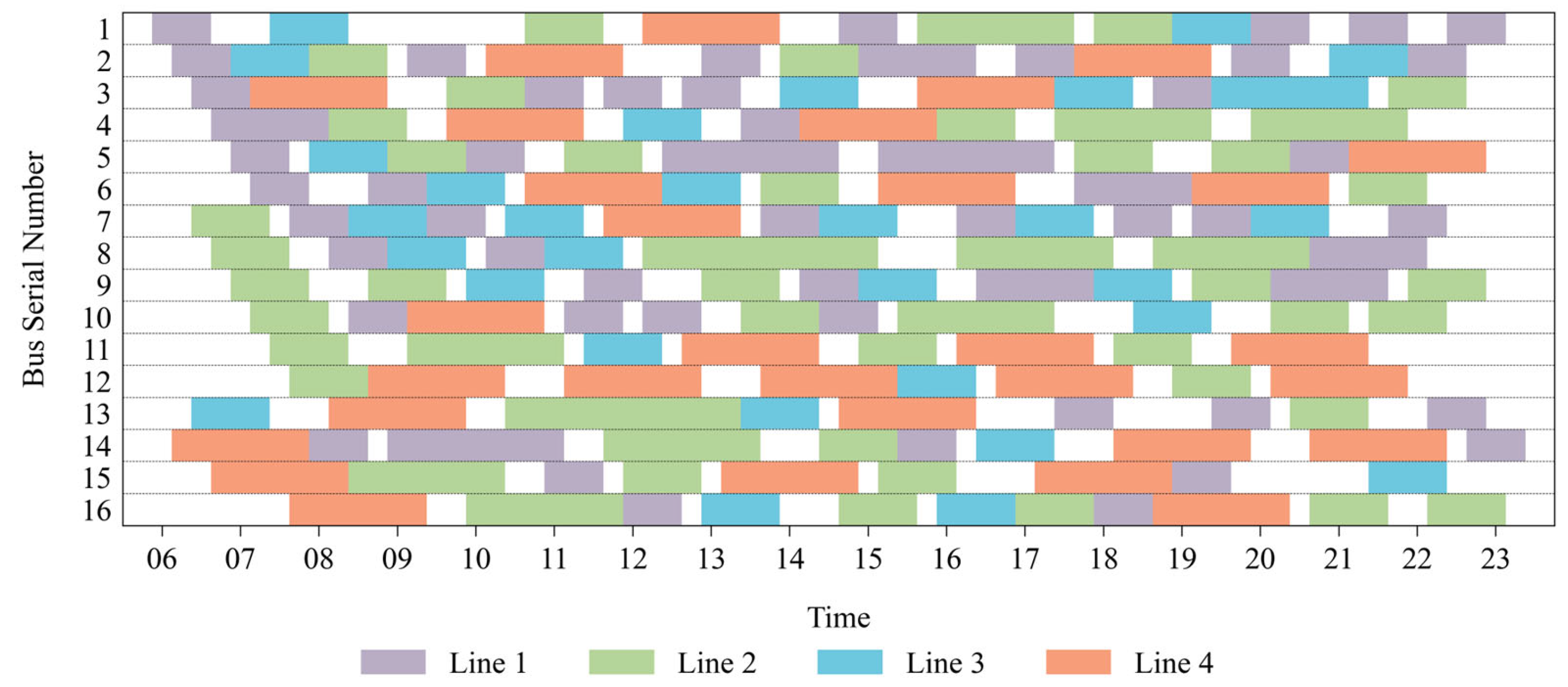
Figure 5 shows that the benefit of fast charging is not uniform across all routes, but is most pronounced on energy-intensive and long-cycle services. Relative to Scenario 1, the reduction in dwell time directly enlarges the feasible task set that a single bus can cover within the operating day. This effect is especially significant for Route 4, where long trip times and high energy consumption previously forced the model to reserve more vehicles under slow charging. Once charging time is compressed, the operational bottleneck shifts from charging duration to timetable connectivity, allowing the same service demand to be met with fewer buses. This indicates that fast charging improves system efficiency not simply by increasing charging power, but by relaxing the time-coupling constraint between successive trips and energy replenishment.

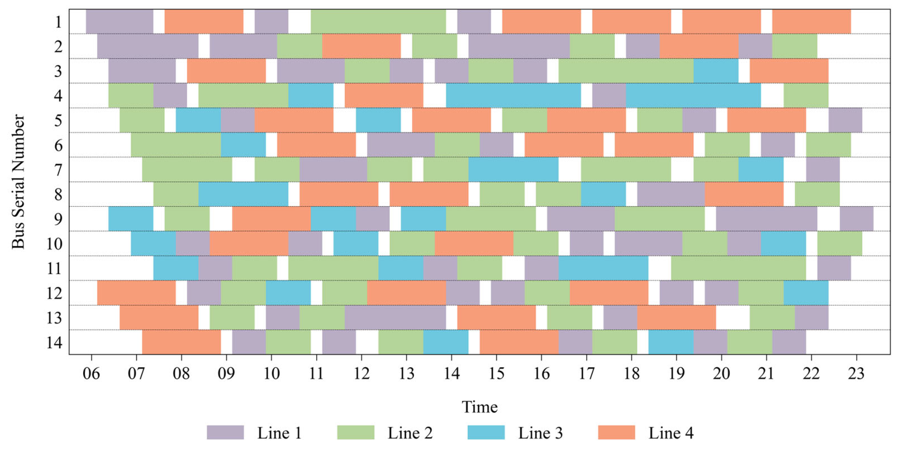
The pattern in Figure 6 indicates that the main contribution of cross-line scheduling lies in converting route-specific idle time into system-wide dispatchable capacity. Under conventional operation, temporal gaps between trips on one route cannot be used to serve demand on another route, even when these gaps are operationally feasible. By allowing route switching, Scenario 3 enables the optimizer to connect trips from different lines into longer and denser task chains, thereby exploiting temporal complementarity across routes. In essence, cross-line scheduling does not reduce service demand itself; instead, it reduces the amount of duplicated reserve capacity required to hedge against route-level temporal mismatches.

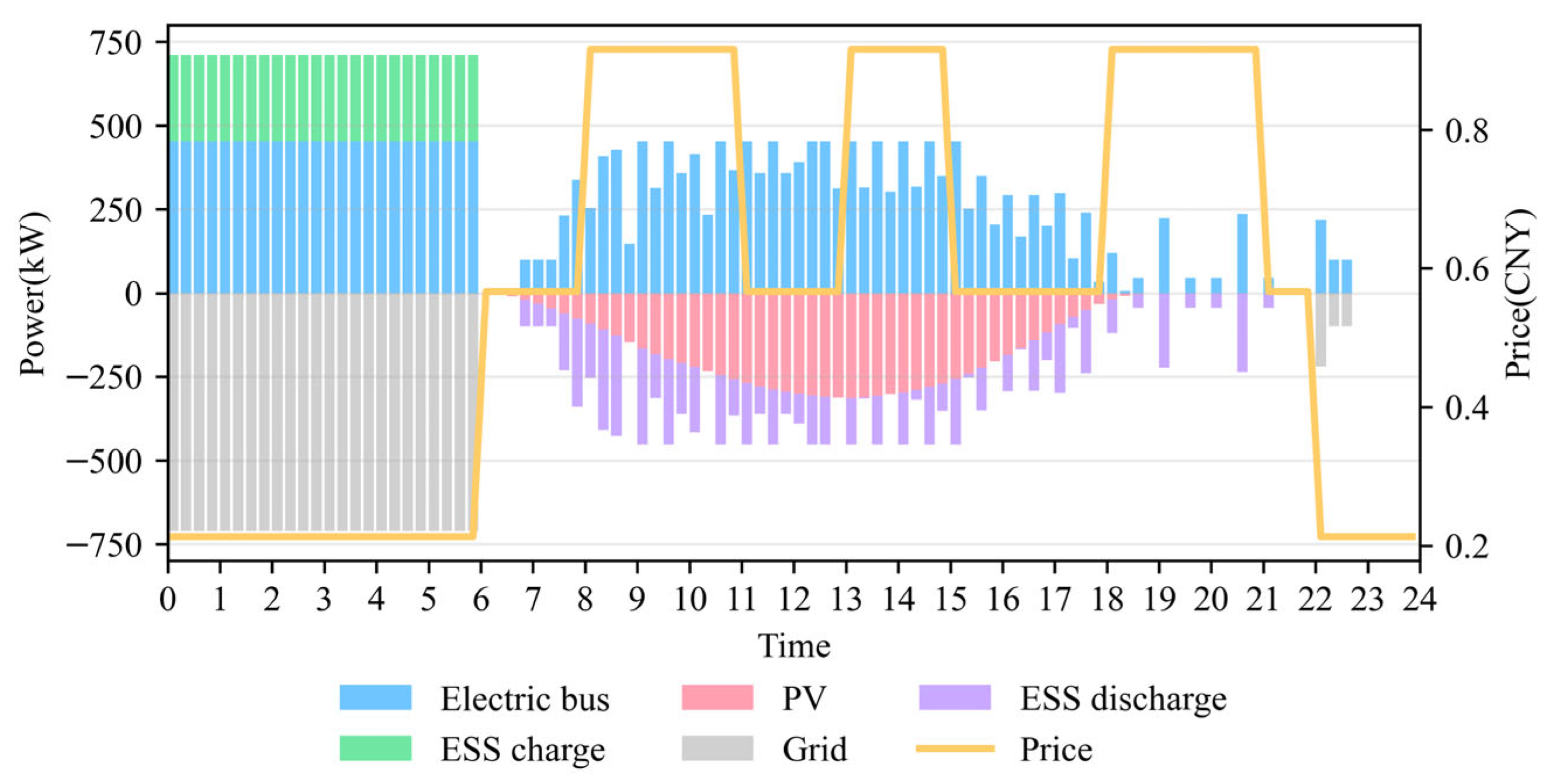
Figure 7 demonstrates the synergistic effect of combining cross-line scheduling with fast charging. Cross-line operation expands the feasible set of task connections across routes, while fast charging shortens the recovery time required between successive duties. When these two mechanisms are implemented simultaneously, the optimizer can construct longer and more compact task chains with fewer interruption periods. Therefore, the improvement observed in Scenario 4 is not a simple sum of the separate benefits seen in Scenarios 2 and 3. Instead, fast charging strengthens the practical value of interlining by increasing the number of cross-route connections that remain energy-feasible, while interlining in turn allows the time saved by fast charging to be translated into actual fleet-size reduction.

3.2.3. Analysis of Charging Station Power Profiles Across Diverse Scenarios

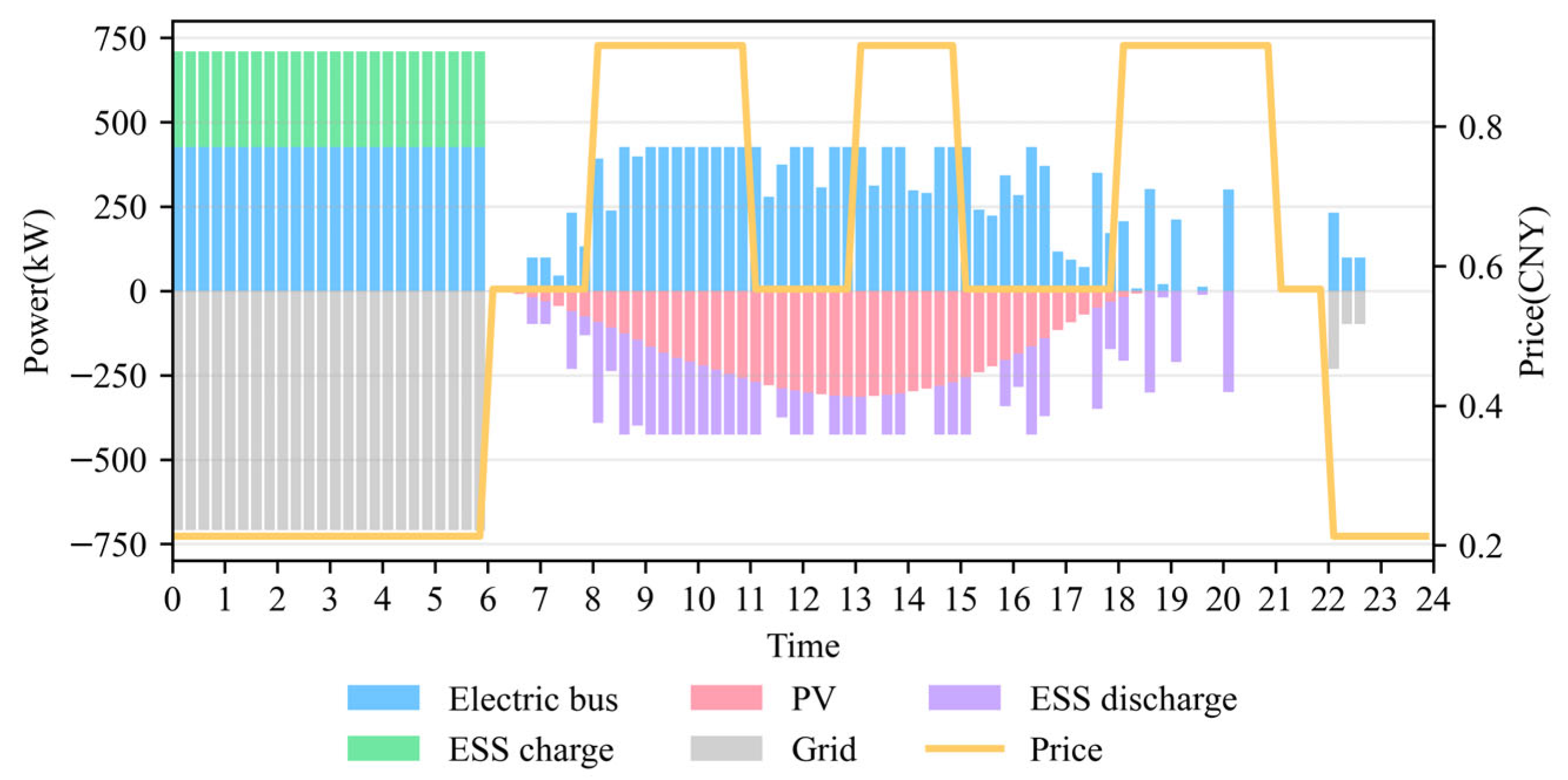
Figure 8 illustrates the power fluctuations of the charging station in Scenario 1. During the period from 0:00 to 6:00, the purchasing power at the bus station remains at a high level. This trend occurs because electricity prices are lower during these hours, encouraging buses and energy storage systems to maintain high state-of-charge levels to satisfy the energy demands of the following day. Consequently, the station minimizes its reliance on the power grid during daytime operations. Throughout the operational hours, the charging requirements of the buses are primarily met by energy storage and PV output. Only after 22:00, when the low-price period begins, do buses draw a small amount of power from the grid to support subsequent energy needs. Scenario 1 achieves lower energy costs by concentrating slow charging for a large number of buses during the nocturnal low-price period, which eliminates the need to purchase electricity from the grid during the day. However, the peak charging load at night reaches approximately 710 kW, resulting in substantial maximum demand costs.

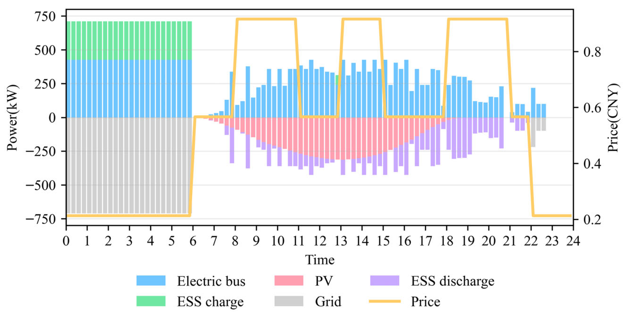
Although Scenarios 2 and 3 exhibit a broadly similar valley-charging pattern to Scenario 1, the underlying drivers differ, as shown in Figure 9 and Figure 10. In Scenario 2, fast charging reduces the duration of individual charging sessions, which improves charger turnover but does not fundamentally change the incentive to concentrate charging during low-tariff hours. In Scenario 3, cross-line scheduling modifies the temporal distribution of vehicle returns to the depot, making charging opportunities more flexible across routes. However, because slow charging is still adopted, the system continues to rely heavily on overnight charging to ensure sufficient energy for the next day.

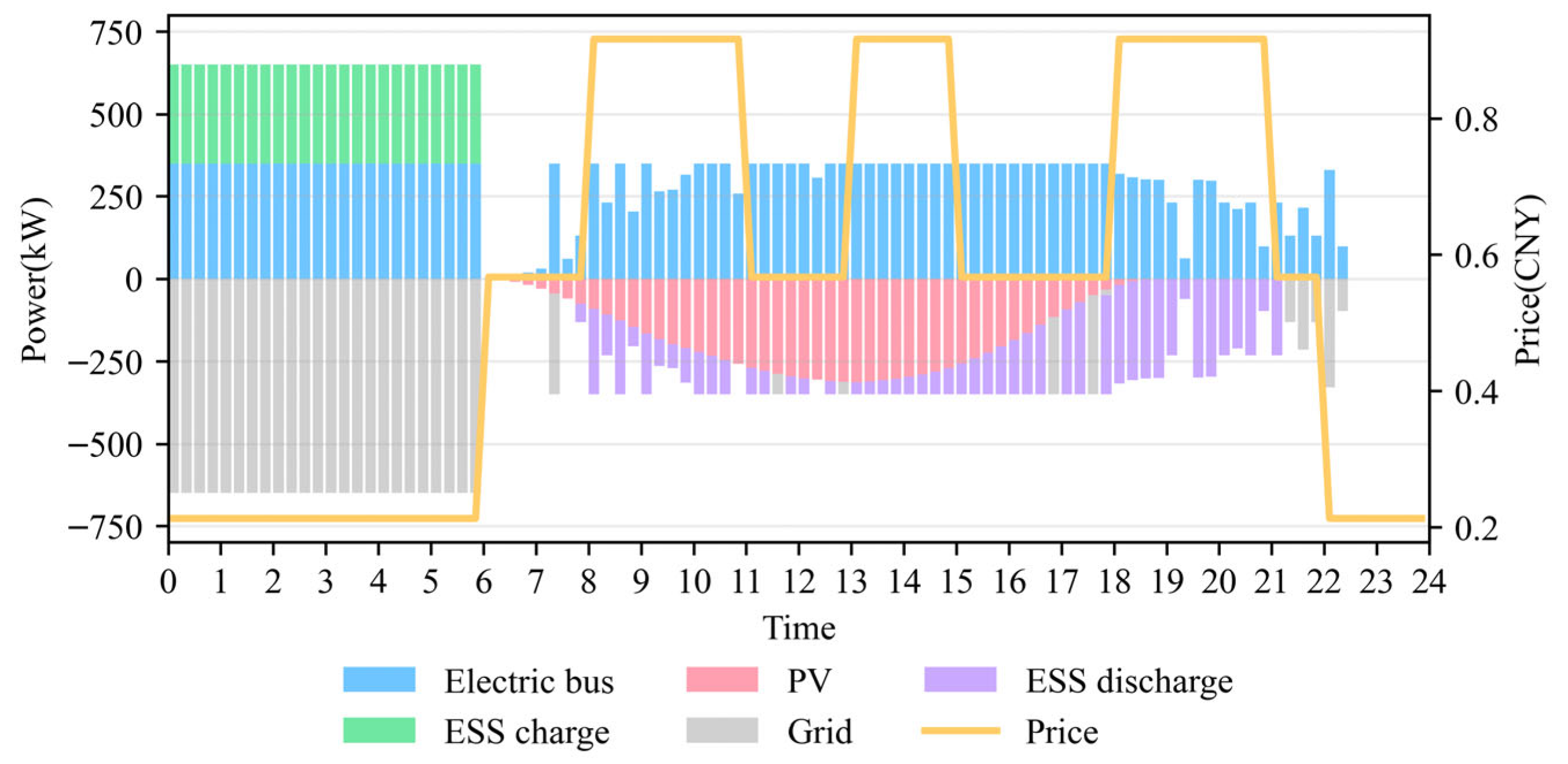
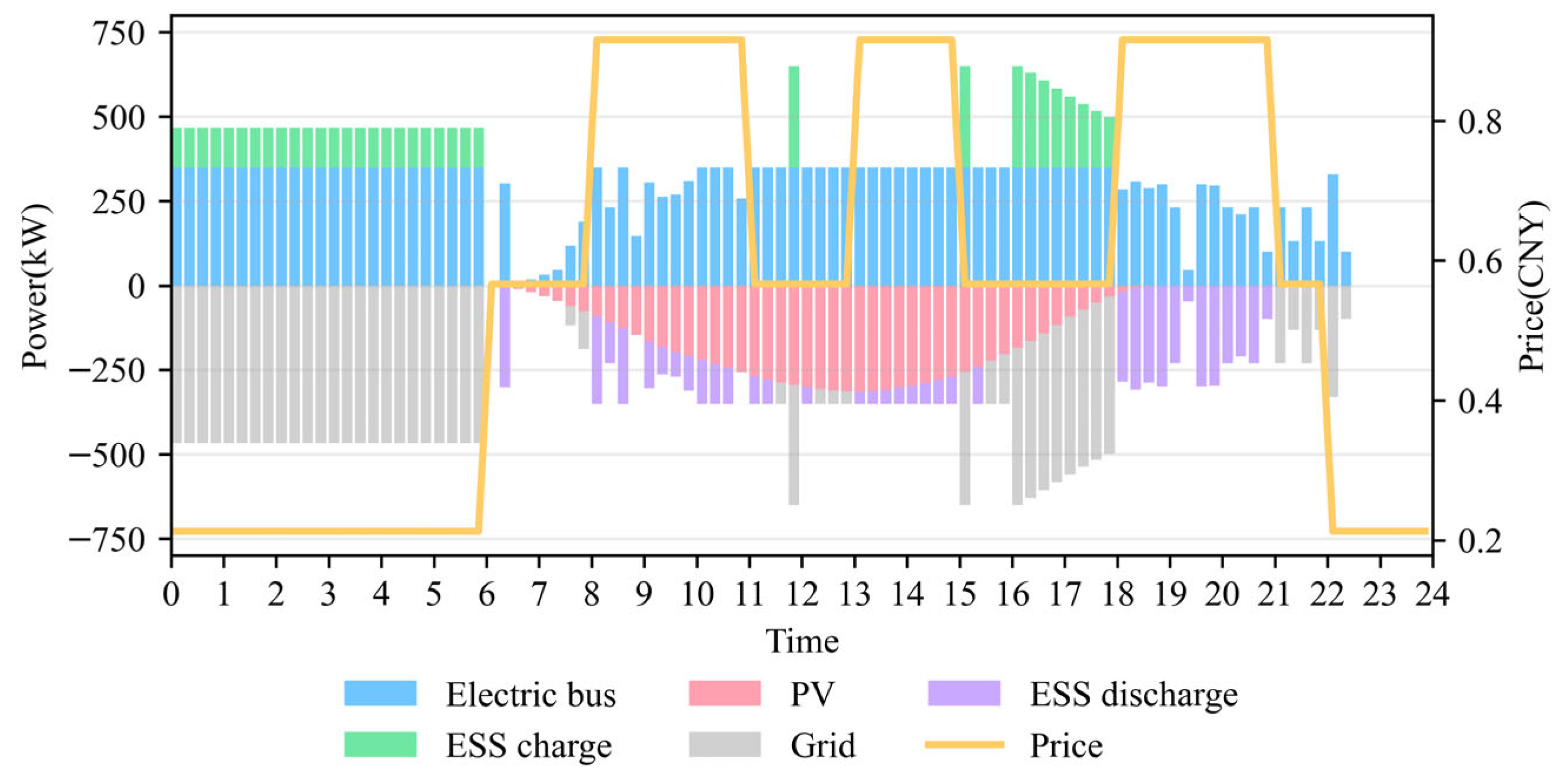
Figure 11 illustrates the power profile of the charging station in Scenario 4. Owing to the reduced fleet size, the peak nighttime charging power decreases to approximately 650 kW, thereby lowering the maximum demand cost. Although the need for supplementary charging during daytime flat-price periods leads to a slight increase in electricity procurement cost, the coordinated operation of PV and energy storage during peak-price periods effectively avoids grid electricity purchases when prices are high. In Scenario 4, the smaller fleet size means that each bus is assigned more transport tasks, which in turn leads to higher average daily energy consumption per bus. As a result, the combination of nighttime charging and PV generation can no longer fully satisfy the total daily energy demand, making additional daytime grid electricity purchases necessary. By contrast, the other scenarios employ larger fleets, which allow transport tasks to be distributed more evenly and result in lower average energy consumption per bus. This enables buses to complete charging and store sufficient energy during low-price nighttime periods to support the entire day of operation, thereby eliminating the need for additional grid electricity purchases during the daytime. As shown in Table 4, the electricity procurement cost in Scenario 4 is higher than that in other scenarios. Nevertheless, Scenario 4 achieves the lowest total system cost by balancing a slight increase in procurement cost against substantial reductions in bus investment, charging infrastructure investment, and maximum demand cost.

4. Discussion

4.1. Integrated Analysis of Joint Scheduling and Charging Strategy

These findings are broadly consistent with recent studies while also highlighting the specific value of the present integrated framework. Existing studies on cross-line or interlining operations have shown that greater route-sharing flexibility can improve vehicle utilization and reduce fleet size [22,23]. Studies on charger planning and charging scheduling have likewise reported that charging power and infrastructure decisions should be coordinated rather than optimized separately [12,14,32]. In addition, recent integrated transportation–energy studies have emphasized the growing importance of jointly considering charging facilities, storage, and broader depot energy systems [17,18,35]. Compared with these studies, the results of this paper further show that when cross-line task chaining and charging mode selection are optimized together with PV–ESS–charger configuration, the benefits are not limited to bus-side fleet reduction, but also extend to charger deployment, demand-charge mitigation, and the overall cost structure of the depot. In particular, the superiority of Scenario 4 indicates that the interaction between operational reorganization and depot energy planning can produce stronger system-level gains than optimizing either side in isolation.

4.2. Sensitivity Analysis of Photovoltaic and Energy Storage Costs

This section investigates how variations in capital costs for PV panels and battery energy storage influence the system’s optimal configuration and economic performance. Using Scenario 4 as the baseline, we conduct a sensitivity analysis by adjusting unit investment costs for PV and storage to observe shifts in optimal installed capacities and charging strategies. The objective is to identify cost threshold effects, such as determining specific PV cost levels where grid reliance outweighs expanding solar capacity. Furthermore, we examine how rising battery costs reduce storage deployment and transition charging patterns from concentrated sessions during valley periods toward more dispersed charging throughout off-peak hours. This analysis clarifies how PV and battery price fluctuations dictate planning decisions, ensuring the robustness and economic viability of configurations under future cost scenarios.

4.2.1. Sensitivity Analysis of Photovoltaic Cost

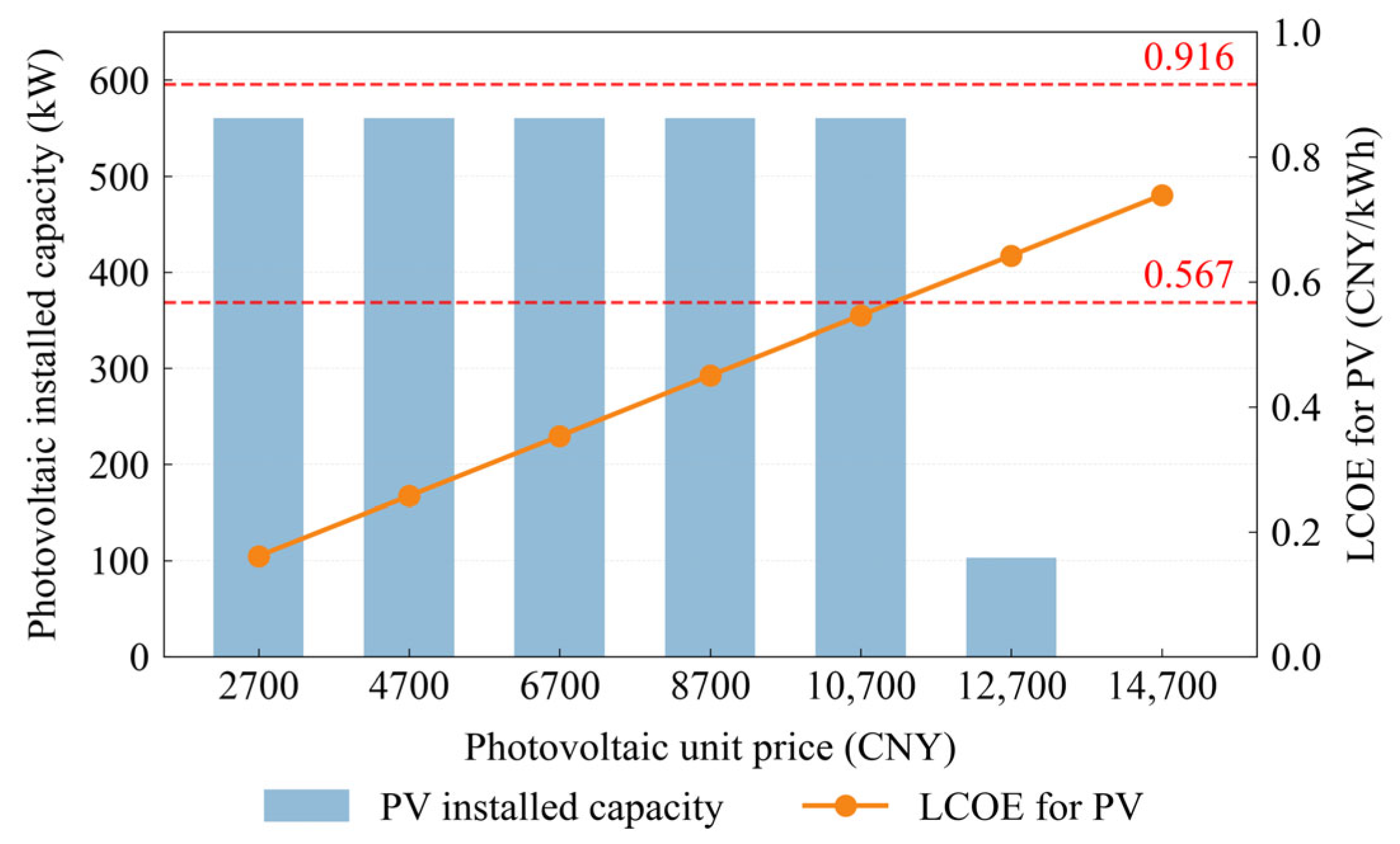
Figure 12 illustrates the variations in installed PV capacity relative to price fluctuations. Changes in the levelized cost of energy (LCOE) for PV trigger adjustments in the optimal installed capacity, revealing a specific economic threshold. When the PV LCOE exceeds 0.567 yuan, the installed capacity begins to decline, and the charging station subsequently increases grid power purchases during parity periods to compensate for the reduction in solar output. The underlying reason is that PV generation concentrates during daylight hours, while the minimum electricity price for grid interaction during the same period is precisely 0.567 CNY. This price serves as the marginal benchmark for comparing PV generation against grid purchases. Once the LCOE surpasses this baseline, the economic advantage of solar power diminishes, prompting the model to gradually reduce the PV installation scale to minimize total system costs. Notably, the optimal capacity does not immediately drop to zero when the LCOE exceeds the electricity price because the cost function incorporates maximum demand charges. A further reduction in capacity forces the station to increase both the power and volume of grid purchases, which potentially raises peak power and elevates maximum demand costs. Consequently, the optimal configuration of PV requires a comprehensive trade-off between solar generation costs and grid maximum demand expenses.

4.2.2. Sensitivity Analysis of Energy Storage Cost

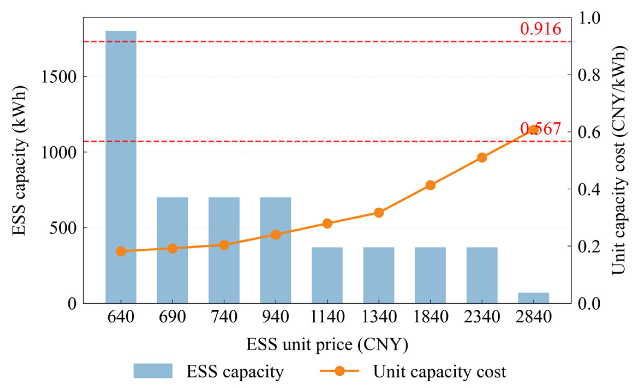
Figure 13 illustrates energy storage capacity variations relative to price fluctuations. Configured capacity remains relatively stable across several cost intervals before declining sharply, indicating strategic shifts at critical price thresholds.

The economic attractiveness of energy storage is determined by the combined effects of three factors: time-of-use arbitrage potential, demand-charge mitigation, and storage investment cost. On the one hand, energy storage enables temporal shifting by charging during valley-price periods and discharging during flat- or peak-price periods, and its arbitrage value depends directly on the electricity price spread. On the other hand, storage operation also reshapes the depot power procurement profile and may either reduce or increase the maximum grid demand, thereby affecting capacity-based electricity charges. Therefore, energy storage becomes economically attractive when it can simultaneously provide sufficient arbitrage revenue and peak-load regulation benefits to offset its capital cost.

This threshold effect can be observed in the case results. When the storage price is relatively low, such as 640 CNY/kWh, the model installs approximately 1800 kWh of storage because large-capacity storage can effectively exploit charging during valley-price periods and discharging during flat- and peak-price periods. Under this condition, the unit energy supply cost is about 0.213 + 0.189 + 0.164 = 0.566 CNY/kWh, which is significantly lower than the flat and peak electricity tariffs, making storage highly economical. However, when the storage price increases to 690 CNY/kWh, the unit energy supply cost rises to 0.213 + 0.189 + 0.174 = 0.576 CNY/kWh. At this point, discharging during flat-price periods no longer provides sufficient marginal benefit, and the role of storage shifts from broad energy arbitrage toward more selective use in high-value peak-price periods. As a result, the optimal storage capacity decreases sharply, which is also reflected in the power variation shown in Figure 14.

As costs rise further, the arbitrage space continues to narrow. When returns fail to cover both equipment investment and the incremental capacity tariffs, marginal economic efficiency drops significantly, leading to further downward adjustments in storage scale. For instance, at a unit price of 1140 CNY/kWh, the optimal configuration capacity decreases markedly, suggesting that large-scale deployment is no longer feasible at this cost level. Overall, energy storage configuration exhibits a stepwise decreasing trend as costs increase, reflecting the dynamic relationship between TOU price spreads, capacity tariffs, and investment costs, which triggers strategic turning points at specific cost thresholds.

4.3. Recommendations and Future Work

Despite the effectiveness of the proposed framework, several directions deserve further study. First, vehicle-to-grid (V2G) technologies could be incorporated to assess the potential of electric bus fleets to provide bidirectional flexibility, such as peak shaving and ancillary services, and to examine their interactions with depot-level storage and charging strategies. Second, the current analysis is limited to a single depot. Extending the model to a multi-depot context would enable coordinated vehicle dispatch and energy sharing across depots, capturing spatial heterogeneity in demand, renewable availability, and grid constraints in large urban bus networks. Incorporating renewable generation uncertainty and real-time operational adjustments would further enhance the robustness and practical applicability of the proposed framework. In future research, degradation cost associated with charging rate, depth of discharge, and operating frequency will be incorporated into the unified optimization framework to improve its long-term economic accuracy and practical applicability.

5. Conclusions

This study develops a coordinated optimization framework for electric bus depots to minimize total costs while satisfying operational and energy constraints. We formulate a MILP model integrating cross-line bus scheduling with PV, energy storage, and charging system configurations. Evaluated using real-world data across four scenarios, the model includes a sensitivity analysis on equipment costs. Several primary conclusions are derived. Integrating cross-line dispatching and fast charging significantly reduces fleet size and infrastructure compared to conventional operations. Scenario analysis demonstrates this joint approach minimizes daily comprehensive costs by offsetting slight increases in electricity procurement with substantial bus and infrastructure savings.

Coordinated energy management shifts charging loads to off-peak periods, reducing maximum demand charges and mitigating peak grid stress. Synergy between nighttime grid charging and daytime PV utilization, supported by energy storage, minimizes reliance on high-tariff electricity. Optimal deployment of PV and energy storage systems exhibits economic thresholds dictated by time-of-use tariffs and capacity charges. Specifically, PV capacity decreases when levelized costs exceed the flat grid price of 0.567 CNY/kWh, while optimal storage capacity declines stepwise as unit investment costs constrain peak-valley arbitrage profitability.

This framework provides transportation planners with a practical tool for designing cost-effective, low-carbon depots by capturing the coupling between bus operations and energy management. A notable limitation is the focus on a single depot and exclusion of bidirectional energy flows. Future research will incorporate vehicle-to-grid technologies for grid flexibility and extend optimization to multi-depot networks considering renewable generation uncertainties.

References

1. UNFCCC. Nationally Determined Contributions Under the Paris Agreement; Synthesis Report by the Secretariat. 2024. Available online: https://unfccc.int/documents/641792 (accessed on 18 November 2025).
2. Zhao, F.; Bai, F.; Liu, X.; Liu, Z. A Review on Renewable Energy Transition under China’s Carbon Neutrality Target. Sustainability 2022, 14, 15006. [Google Scholar] [CrossRef]
3. Zhao, F.; Liu, X.; Zhang, H.; Liu, Z. Automobile Industry under China’s Carbon Peaking and Carbon Neutrality Goals: Challenges, Opportunities, and Coping Strategies. J. Adv. Transp. 2022, 2022, 5834707. [Google Scholar] [CrossRef]
4. Lei, X.; Zhong, J.; Chen, Y.; Shao, Z.; Jian, L. Grid Integration of Electric Vehicles within Electricity and Carbon Markets: A Comprehensive Overview. eTransportation 2025, 25, 100435. [Google Scholar] [CrossRef]
5. Ministry of Transport of the People’s Republic of China. Statistical Bulletin on the Development of the Transportation Industry in 2024; Ministry of Transport of the People’s Republic of China: Beijing, China, 2025. Available online: https://xxgk.mot.gov.cn/2020/jigou/zhghs/202506/t20250610_4170228.html (accessed on 18 November 2025).
6. Alamatsaz, K.; Hussain, S.; Lai, C.; Eicker, U. Electric Bus Scheduling and Timetabling, Fast Charging Infrastructure Planning, and Their Impact on the Grid: A Review. Energies 2022, 15, 7919. [Google Scholar] [CrossRef]
7. Liu, Z.; Ma, X.; Zhuo, S.; Liu, X. Optimizing Shared Charging Services at Sustainable Bus Charging Hubs: A Queue Theory Integration Approach. Renew. Energy 2024, 237, 121860. [Google Scholar] [CrossRef]
8. Liu, X.; Plötz, P.; Yeh, S.; Liu, Z.; Liu, X.C.; Ma, X. Transforming Public Transport Depots into Profitable Energy Hubs. Nat. Energy 2024, 9, 1206–1219. [Google Scholar] [CrossRef]
9. Liu, X.; Yeh, S.; Plötz, P.; Ma, W.; Li, F.; Ma, X. Electric bus charging scheduling problem considering charging infrastructure integrated with solar photovoltaic and energy storage systems. Transp. Res. Part E 2024, 187, 103572. [Google Scholar] [CrossRef]
10. Ji, Y.; Zhang, X.; He, P.; Wang, S.; Liu, X.; Li, C. Optimization Configuration of the Whole Life Cycle of Photovoltaic and Storage System Considering Carbon Emission and Improved Line Loss Rate Calculation Model. Electr. Power Syst. Res. 2026, 252, 112383. [Google Scholar] [CrossRef]
11. Barzegari, V.; Nourinejad, M. Transit Electrification through Charger Deployment, Fleet Type Selection, and Charging Schedule Optimization. Energy 2025, 340, 139181. [Google Scholar] [CrossRef]
12. Najafi, A.; Gao, K.; Parishwad, O.; Tsaousoglou, G.; Jin, S.; Yi, W. Integrated Optimization of Charging Infrastructure, Electric Bus Scheduling and Energy Systems. Transp. Res. Part D Transp. Environ. 2025, 141, 104664. [Google Scholar] [CrossRef]
13. Adar, M.; Babay, M.A.; Boussif, M.; Khaouch, Z.; Abbassi, Z.; Najih, Y.; Mabrouki, M. Optimization of Photovoltaic System Modelling: A Comparative Study and Experimental Validation Using Bond Graph Methodology and a Genetic Algorithm. In Applied Mathematics, Modeling and Computer Simulation; IOS Press: Amsterdam, The Netherlands, 2024; pp. 723–730. [Google Scholar] [CrossRef]
14. Gkiotsalitis, K.; Rizopoulos, D.; Merakou, M.; Iliopoulou, C.; Liu, T.; Cats, O. Electric bus charging station location selection problem with slow and fast charging. Appl. Energy 2025, 382, 125242. [Google Scholar] [CrossRef]
15. Zhou, Y.; Wang, H.; Wang, Y.; Liu, R. Robust Optimization for Integrated Planning of Electric-Bus Charger Deployment and Charging Scheduling. Transp. Res. Part D Transp. Environ. 2022, 110, 103410. [Google Scholar] [CrossRef]
16. Wang, X.; Song, Z.; Xu, H.; Wang, H. En-Route Fast Charging Infrastructure Planning and Scheduling for Battery Electric Bus Systems. Transp. Res. Part D Transp. Environ. 2023, 117, 103659. [Google Scholar] [CrossRef]
17. Fan, S.; Zhang, W.; Li, Y.; Shi, J.; Guo, Z.; Bao, Y. Joint Optimization of Bus Fast-Charging Station and Energy Storage Sizing Considering the Variation of Energy Conversion Efficiency. Electr. Power Syst. Res. 2026, 250, 112132. [Google Scholar] [CrossRef]
18. Wang, Y.; Liao, F.; Bi, J.; Liu, R. Optimal Battery Electric Bus System Planning Considering Heterogeneous Vehicles, Opportunity Charging, and Battery Degradation. Renew. Energy 2024, 237, 121596. [Google Scholar] [CrossRef]
19. Zhou, Y.; Wang, H.; Wang, Y.; Yu, B.; Tang, T. Charging facility planning and scheduling problems for battery electric bus systems: A comprehensive review. Transp. Res. Part E 2024, 183, 103463. [Google Scholar] [CrossRef]
20. Bunte, S.; Kliewer, N. An Overview on Vehicle Scheduling Models. Public Transp. 2009, 1, 299–317. [Google Scholar] [CrossRef]
21. Weng, J.; Wang, M.; Lin, P.; Ma, S.; Xu, L.; Liang, F. Cross-line Combined Bus Scheduling Optimization Method Based on Passenger Flow Characteristic Identification. J. South China Univ. Technol. (Nat. Sci. Ed.) 2022, 50, 39–48. (In Chinese) [Google Scholar] [CrossRef]
22. Keshavarzian, K.; Moradi Amani, A.; Jalili, M. Optimal Fleet Size for Cross-Route Dispatching in Electrified Bus Networks. IEEE Trans. Netw. Sci. Eng. 2024, 11, 1567–1579. [Google Scholar] [CrossRef]
23. Li, X.; Zhang, S.; Yuan, Y. Multi-Line Cooperative Cross-Line Bus Dispatch Optimization under Time-Varying Environment. J. Transp. Eng. Inf. 2025, 23, 119–134. (In Chinese) [Google Scholar] [CrossRef]
24. Gao, W.; Lu, S.; Zhao, Y.; Liu, K. Integrated Optimization of Electric Bus Timetabling and Vehicle Scheduling Considering Segmented Charging Strategies. J. Transp. Syst. Eng. Inf. Technol. 2025, 25, 239–248. (In Chinese) [Google Scholar] [CrossRef]
25. Gkiotsalitis, K.; Wu, Z.; Cats, O. A Cost-Minimization Model for Bus Fleet Allocation Featuring the Tactical Generation of Short-Turning and Interlining Options. Transp. Res. Part C Emerg. Technol. 2019, 98, 14–36. [Google Scholar] [CrossRef]
26. Bie, Y.; Qin, W.; Wu, J. Optimal electric bus scheduling method under hybrid energy supply mode of photovoltaic-energy storage system-power grid. Appl. Energy 2024, 372, 123774. [Google Scholar] [CrossRef]
27. Wang, C.; Song, Y.; Fan, G.; Jin, H.; Su, L.; Zhang, F.; Wang, X. Optimizing Cross-Line Dispatching for Minimum Electric Bus Fleet. IEEE Trans. Mob. Comput. 2021, 22, 2307–2322. [Google Scholar] [CrossRef]
28. Jiang, M.; Zhang, Y. A Branch-and-Price Algorithm for Large-Scale Multidepot Electric Bus Scheduling. IEEE Trans. Intell. Transp. Syst. 2022, 24, 15355–15368. [Google Scholar] [CrossRef]
29. Liang, J.; Zhuang, C.; Liu, H.; Gao, Z. Demand-Driven Timetabling and Vehicle Scheduling Optimization for Electric Bus Transit Lines. Transp. Res. Part C Emerg. Technol. 2026, 183, 105482. [Google Scholar] [CrossRef]
30. Duan, M.; Liao, F.; Qi, G.; Guan, W. Integrated Optimization of Electric Bus Scheduling and Charging Planning Incorporating Flexible Charging and Timetable Shifting Strategies. Transp. Res. Part C Emerg. Technol. 2023, 152, 104175. [Google Scholar] [CrossRef]
31. Lu, Z.; Xing, T.; Li, Y. Optimization of Electric Bus Vehicle Scheduling and Charging Strategies under Time-of-Use Electricity Price. Transp. Res. Part E Logist. Transp. Rev. 2025, 196, 104021. [Google Scholar] [CrossRef]
32. Zeng, Z.; Wang, S.; Qu, X. Consolidating Bus Charger Deployment and Fleet Management for Public Transit Electrification: A Life-Cycle Cost Analysis Framework. Engineering 2023, 21, 45–60. [Google Scholar] [CrossRef]
33. Wang, Y.; Liao, F.; Lu, C. Integrated Optimization of Charger Deployment and Fleet Scheduling for Battery Electric Buses. Transp. Res. Part D Transp. Environ. 2022, 109, 103382. [Google Scholar] [CrossRef]
34. Liu, J.; Zhang, J.; Dong, C.; He, Q. Optimizing Battery Electric Bus Allocations: An Integrated Approach to Cost Minimization and Evolutionary Game Theory. Transp. Lett. 2025, 18, 636–669. [Google Scholar] [CrossRef]
35. Ma, X.; Ma, W.; Tao, Y.; Gao, K.; Liu, X. Optimizing bus charging infrastructure by incorporating private car charging demands and uncertain solar photovoltaic generation. npj Sustain. Mobil. Transp. 2025, 2, 6. [Google Scholar] [CrossRef]
36. China Photovoltaic Industry Association. 2024–2025 China Photovoltaic Industry Development Roadmap. 2025. Available online: https://www.chinapv.org.cn/Industry/resource_1405.html (accessed on 18 November 2025).
37. Xiao, G.; Xiao, Y.; Shu, Y.; Ni, A.; Jiang, Z. Technical and economic analysis of battery electric buses with different charging rates. Transp. Res. Part D Transp. Environ. 2024, 132, 104254. [Google Scholar] [CrossRef]
38. National Center for Climate Change Strategy and International Cooperation. National Greenhouse Gas Emission Factor Database (First Edition). 2025. Available online: https://data.ncsc.org.cn/factories/index (accessed on 6 February 2026).
39. Consortium Led by the Solar Energy Research Institute of Singapore (SERIS). UPDATE of the Solar Photovoltaic (PV) Roadmap for Singapore [R/OL]. March 2020. Available online: https://www.seris.nus.edu.sg/wp-content/uploads/2023/07/Update-of-the-Solar-Roadmap-for-Singapore-March-2020.pdf (accessed on 18 November 2025).
Figure 1. Typical bus charging station model.
Energies 19 01791 g001
Figure 2. Charging stations under cross-line operation.
Energies 19 01791 g002
Figure 3. Algorithm Flowchart for Problem Solving.
Energies 19 01791 g003
Figure 4. The detailed daily operational schedule obtained for Scenario 1.
Energies 19 01791 g004
Figure 5. The detailed daily operational schedule obtained for Scenario 2.
Energies 19 01791 g005
Figure 6. The detailed daily operational schedule obtained for Scenario 3.
Energies 19 01791 g006
Figure 7. The detailed daily operational schedule obtained for Scenario 4.
Energies 19 01791 g007
Figure 8. Power status of charging stations in Scenario 1.
Energies 19 01791 g008
Figure 9. Power status of charging stations in Scenario 2.
Energies 19 01791 g009
Figure 10. Power status of charging stations in Scenario 3.
Energies 19 01791 g010
Figure 11. Power status of charging stations in Scenario 4.
Energies 19 01791 g011
Figure 12. Configuration under different photovoltaic prices.
Energies 19 01791 g012
Figure 13. Configuration under different energy storage prices.
Energies 19 01791 g013
Figure 14. Charging power profile of the depot under a storage unit cost of 690 CNY/kWh.
Energies 19 01791 g014