SCADA Data-Driven Remaining Useful Life Estimation of Wind Turbine Generators

Abstract

Generator faults are among the most expensive events in utility-scale wind turbines, and the remaining useful life (RUL) of a generator is strongly influenced by long-term thermal loading on windings and bearings. Although wind farms continuously log multi-point generator temperatures and operating variables via SCADA, these data are rarely converted into an actionable, quantitative RUL trajectory that can be used directly for maintenance planning. This study proposes a field-oriented RUL estimation framework that transforms multi-year SCADA records into degradation-focused indicators and converts them into a physically plausible, decision-ready RUL curve. First, SCADA data are cleaned and filtered by operating conditions, and temperature rises relative to ambient are extracted. Next, abnormal operation is detected and summarised using an abnormal operation index (AOI), and thermal severity indicators are aggregated into a health index (HI) that reflects both proximity to engineering limits and signal variability. The HI is then mapped to lifetime consumption to update an effective age relative to the generator’s designed lifetime, followed by smoothing and monotonicity enforcement to ensure a stable, non-increasing RUL trajectory. Field validation shows a highly smooth RUL profile (98.2%) and a near-linear long-term decreasing trend ($R^2=0.985$). The results demonstrate that SCADA temperature–operation data can support reliable online generator RUL prognostic monitoring without the need for additional sensors.

1. Introduction

Wind energy has become one of the most rapidly expanding renewable energy sources worldwide, driven by the demand for low-carbon electricity generation. As wind turbine fleets age and scale up, operation and maintenance (O&M) costs increasingly dominate the total cost of energy [1]. Among turbine subsystems, the generator is a high-value, mission-critical component, with unexpected failures often resulting in prolonged downtime, costly repairs, and substantial revenue losses. Consequently, the ability to predict the remaining useful life (RUL) of wind turbine generators has become a key enabler for condition-based maintenance and long-term asset management strategies [2]. In practical operation, generator degradation is strongly associated with long-term thermal loading of windings, insulation systems, and bearings. Elevated temperatures and repeated thermal cycling accelerate insulation ageing and material fatigue, ultimately reducing the effective lifetime of the generator. Modern wind turbines continuously record multiple generator temperature signals—such as stator winding, bearing, and cooling system temperatures—through supervisory control and data acquisition (SCADA) systems. These multi-point thermal measurements provide valuable, yet often underutilised, information on cumulative thermal stress and operational severity, making SCADA-based temperature data a promising foundation for generator RUL modelling.

One of the main factors influencing generator ageing is thermal loading: bearings and structural components are affected by frictional heating, lubrication conditions, and local hot spots, while stator windings’ cumulative exposure to high temperatures and thermal cycling accelerate insulation degradation. In addition to operating factors like power, speed, and wind conditions, which implicitly carry information regarding lifespan consumption, modern turbines continually record generator temperatures [3]. However, the majority of prognostics and health-management studies in the literature still concentrate on gearboxes and main bearings, and these measures are mostly employed in contemporary industrial practice for threshold-based protection and straightforward trend graphs [4,5]. This creates a gap for generator-focused RUL models that provide RUL trajectories that are both physically and statistically feasible for direct use in maintenance planning, while clearly connecting long-term temperature and operation histories to lifetime utilisation [6,7].

Numerous studies have used temperature and operating data for RUL at the drivetrain level, but primarily focus on bearings or gearboxes [8,9]. For wind turbine bearings, Hu et al. proposed a performance degradation model and real-time RUL prediction based on temperature, using smoothed temperature series and a Wiener process with an inverse Gaussian RUL distribution; this provides a sound probabilistic framework and accounts for wind-condition uncertainty, but the target is only the bearing and a single temperature channel, without addressing generator ageing or the long-term temperature–operation–design-life link [10]. Rezamand et al. improved bearing RUL by clustering operating conditions using kernel fuzzy C-means and building regime-specific adaptive models, highlighting the importance of handling varying operating regimes; however, the method remains limited to drivetrain bearings, relies on well-labelled degradation data, and does not address the generator’s long-horizon RUL behaviour [11]. More recently, Vieira et al. proposed a main-bearing RUL framework based on monitoring-system temperatures, using regression models on raw bearing temperatures to estimate RUL in two real wind farms. However, it uses only operational data and relies on a single bearing temperature channel. It does not analyse in detail the shape of the RUL trajectory or its response to abnormal phases [12]. Other predictive-maintenance works for main bearings use ambient temperature, rotor speed, and power to detect anomalies, but typically stop at risk/status classification rather than constructing long-term, design-life-related RUL trajectories [13].

For gearbox RUL, Carroll et al. used SCADA data and vibration data with machine learning models to predict failures and RUL, achieving good accuracy but at the cost of additional sensors and large, labelled datasets, and without explicitly targeting a smooth, near-linear RUL trajectory [14]. More recent works define temperature-based indices from long-term operating data to estimate end-of-life for drivetrain and generator bearings. Yet, the authors note that RUL from routine data alone remains highly uncertain and should be treated only as a supporting indicator [15,16]. At generator level, Schamboeck et al. classified anomalies, mapped them to a health index, and extrapolated this index with ARIMA to a failure threshold, thus using existing data but inferring RUL only indirectly, without an explicit temperature–operation–design-life link or analysis of RUL-curve properties [17]. These limitations motivate a generator RUL model that exploits available temperature and operating data while explicitly checking the shape and consistency of the RUL trajectory against the machine’s designed lifetime [18,19].

In this study, the term “online prognostics” refers to the continuous updating of the generator RUL trajectory as new SCADA data become available. The proposed framework is intended for long-term health monitoring and maintenance planning, rather than instantaneous transient-fault detection. Therefore, the RUL output is updated in an online causal manner using historical observations only. Rather than focusing on fault detection or short-term anomaly flags, the objective is to construct an RUL trajectory that reflects the generator’s long-term consumption over its designed lifetime and can be used directly for maintenance planning. Historical generator temperatures and operating variables are treated as a degradation signal, and an RUL model is formulated to map these time histories to the remaining calendar time until primary generator intervention. Emphasis is placed on ensuring that the RUL trajectory is physically plausible: monotonically decreasing on average, sensitive to abnormal thermal behaviour, and consistent with the nominal design lifetime over the observation period.

Operationally, multi-year temperature and operating records are first preprocessed by removing non-representative states, filtering outliers, and normalising temperatures with respect to ambient or nacelle conditions. The cleaned data are then converted into degradation-oriented series by isolating regular production periods and expressing thermal behaviour as temperature rises and long-term trends under comparable loading. Using the designed lifetime curve, a time-to-end-of-life label is assigned to each observation, and an RUL model is constructed that compares observed thermal usage against this design curve to obtain a calendar-time RUL trajectory. This trajectory is evaluated using quantitative criteria such as day-to-day stability, responsiveness to thermally abnormal episodes, and long-term linearity between predicted RUL and calendar time. In the representative generator case study, the model yields a smooth, strictly decreasing RUL curve that closely follows the expected design-lifetime consumption with a R-squared value $R^2\approx 0.985$ for a linear fit, accelerates appropriately during abnormal thermal periods, and remains stable otherwise. These properties provide operators with an interpretable, calendar-time RUL signal that is both numerically robust and physically credible, enabling proactive generator maintenance based on actual thermal usage rather than only fixed schedules or post-fault actions.

2. The Study Wind Turbine Description and Data

2.1. Overview of the Wind Turbine Generator Specifications and SCADA Data

The proposed RUL framework is applied to a modern 2 MW onshore variable-speed wind turbine with a conventional three-stage drivetrain, typical of current industrial fleets. Aerodynamic torque from the rotor is transmitted through the main shaft and gearbox to the generator shaft, where mechanical power is converted into electrical power and exported to the medium-voltage collection grid via a step-up transformer and switchgear. In this power range, the generator is implemented as a doubly fed induction generator (DFIG) with a wound rotor and a partially rated back-to-back converter. The machine is designed for continuous operation over a wide speed range and for a nominal design lifetime of approximately 20 years under specified thermal and mechanical loading conditions. This design lifetime later serves as the reference curve against which field thermal usage and the estimated RUL trajectory are interpreted.

From a condition-monitoring perspective, the generator is one of the most critical drivetrain components, entirely consistent with the motivation outlined in the Introduction. Thermal stress on the stator windings governs insulation ageing and, in turn, the probability of winding failure. At the same time, the bearings and generator frame are influenced by frictional heating, lubrication state, and possible shaft misalignment. To manage these risks in the field, the DFIG is instrumented with multiple embedded temperature sensors at thermally sensitive locations, and over-temperature limits are enforced in the turbine control system to issue alarms or trigger protective shutdowns. All these signals, along with ambient/nacelle temperature, generator speed, active power, and turbine state flags, are recorded by the SCADA system at 10 min resolution and serve as the basis for the field-based RUL analysis.

Table 1. Specifications of the 2 MW wind turbine generator.

Parameter	Symbol	Value
Rated power	$P_{rated}$	2 MW
Cut-in/out wind speed	$W_{{\displaystyle \frac{in}{out}}}$	3~25 m/s
Rated wind speed	$W_{rated}$	11 m/s
Rated line voltage	$U_{rated}$	690 V (AC, three-phase)
Generator type	-	Doubly fed induction generator (DFIG)
Speed range (mechanical)	${\omega }_{mech}$	≈700–1400 rpm (variable speed)
Cooling method	-	Cooling through a water jacket
Stator insulation class	-	Class F or higher
Nominal design lifetime	$L_{design}$	≈20 years
SCADA logging interval	Δt	10 min averages

summarises the key specifications of the 2 MW DFIG used in this study (rated power, voltage, speed range, insulation class, cooling method, etc.). These values provide the design context for defining allowable temperature rises, interpreting thermal indicators, and quantifying lifetime consumption in the subsequent sections.

A central SCADA system supervises all turbines in the wind farm. At each turbine, a PLC samples electrical, mechanical, and environmental signals (typically at around 1 Hz or higher internally) and aggregates them into 10 min averaged values for storage in the SCADA database. For every 10 min interval, the system records the average of a predefined set of variables that includes:

• Generator-related temperatures: stator winding phase temperatures (U, V, and W), drive-end and non-drive-end bearing temperatures, and generator frame/housing temperature.
• Operating variables: generator active power, generator speed (and rotor speed if available), nacelle wind speed, ambient/nacelle air temperature, pitch angle, and yaw position.
• Status information: turbine operating state (normal production, curtailed operation, start-up, shutdown, fault, and maintenance), together with alarm and event logs (e.g., over-temperature alarms, generator fault codes, and trips).

Over the multi-year horizon considered in this study, this architecture yields long, regular multivariate time series for each 2 MW DFIG turbine, with a uniform 10 min sampling interval. For the generator RUL analysis, turbines with at least one documented generator repair or replacement event are selected. For each selected unit, all relevant temperature and operating variables, along with time-stamped alarms and maintenance records, are extracted from the SCADA database and merged into a single, time-aligned dataset at 10 min intervals. This results in several hundred thousand data points spanning multiple years of operation, capturing seasonal and operational variability, as well as the gradual thermal behaviour leading up to the generator intervention. These datasets form the basis for preprocessing, operating-condition filtering, and RUL model construction described in the subsequent sections.

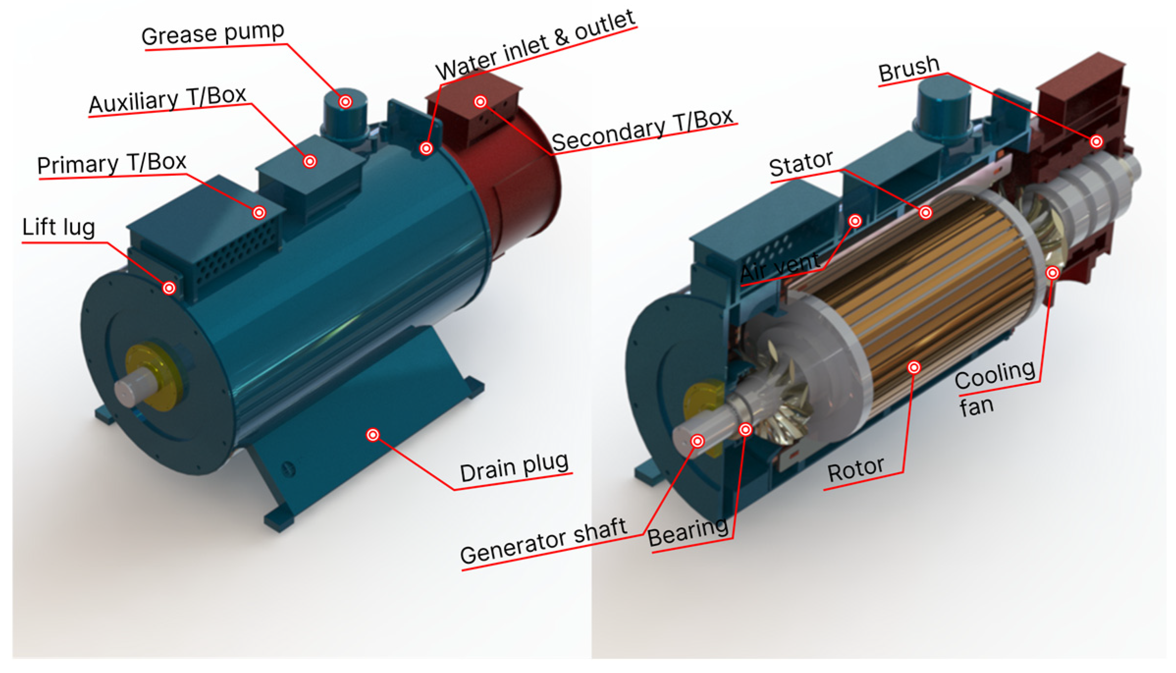
Figure 1 illustrates the main structural elements of the 2 MW DFIG used in this study. The external view shows the primary and auxiliary terminal boxes, the secondary terminal box for the rotor circuit, the grease pump, lifting lugs, and the water inlet/outlet ports for the cooling system. The cut-away view reveals the internal components, including the stator core and windings fixed to the frame, the rotor mounted on the generator shaft, the drive-end and non-drive-end bearings, and the shaft-mounted cooling fan and air vents that guide the airflow through the machine. Brushes and the rotor terminal box connect the wound rotor to the back-to-back converter. In practice, resistance-temperature detectors are embedded near the stator windings, bearings, and frame surfaces shown in Figure 1; these locations correspond directly to the temperature channels listed in

Table 2. Generator-related input variables, normal ranges.

Data Type	Normal Data Range	Unit	Value
Gen. bearing (drive end) temperature	40~75	°C	Grease life halves every ~15 °C; >105 °C risks cage and lubricant failure; compare DE vs. NDE ΔT to detect misalignment.
Gen. bearing (non-drive end) temperature	40~75	°C	Same thermal limits as drive end (grease and races).
Gen. winding temperature [U, V, W]	40~90	°C	Class F insulation ~155 °C hot-spot; alarms below trip protect ageing margin; U/V/W should be balanced, ΔT > 10 °C suggests cooling imbalance.
Environment temperature	−10~45	°C	Most components specified for IEC climate class; extreme temperatures reduce cooling and material margins; cold-climate kits may extend the low-temperature range.
Wind speed	3~25	m/s	Defined by the power curve and structural loads, the controller stops above cut-out; gusts may trigger early shutdowns.
Active power	0~2	MW	Tracks controller setpoint and grid code requirements; persistent deviation indicates faults or derating; max rated ≈ 2 MW.
Generator speed	0.7~1.1	Rpm	Overspeed margins set by drivetrain and rotor design; converters/governors limit to protect mechanicals.

and to the SCADA data streams later used to construct the thermal indicators and lifetime-usage model.

In the generator RUL model, a subset of SCADA channels was selected that directly reflects generator thermal loading and the corresponding operating conditions. The chosen variables, their typical normal operating ranges, and indicative abnormal thresholds are summarised in Table 2. The temperature channels include drive-end and non-drive-end bearing temperatures and stator winding temperatures for the three phases (U, V, and W). Under regular operation, bearing temperatures are expected to remain in the range of approximately 40–90 °C; alarm and trip thresholds are set at about 95 °C and 105 °C, respectively, reflecting the rapid reduction in grease life with increasing temperature and the risk of cage or lubricant damage at elevated temperatures. Stator winding temperatures typically range from 80 °C to 130 °C, with alarms issued above 140 °C and trips above 155 °C, consistent with the hot-spot limit for Class F insulation. Persistent deviations between phase temperatures are used as indicators of cooling imbalance or local hot spots. The environment (nacelle) temperature channel, with a standard range of −20–45 °C, is used both as a reference for computing temperature rises and as a constraint on cooling performance; alarms are set below −25 °C or above 50 °C, and derating or trip actions may occur if temperatures fall below −30 °C or exceed 55 °C.

The model’s operating variables include wind speed, generator active power, and generator speed. Wind speed values between roughly 3 and 25 m/s cover cut-in, rated, and cut-out operation, with the controller enforcing shutdown above cut-out to protect the rotor and structure. Active power spans from 0 to 2 MW, corresponding to the full range from standstill to rated power; deviations greater than approximately 5–10% from the commanded setpoint, or persistent curtailment at lower levels, are interpreted as potential indications of derating or faults and are logged as abnormal behaviour. Generator speed is expressed in per-unit of the rated speed, with a typical normal range of 0.7–1.1 pu; overspeed protection is configured with alarms above about 1.15 pu and trips above 1.25 pu, values consistent with drivetrain and rotor design margins for a 2 MW DFIG (typically ~600–1400 rpm depending on the number of poles). These thresholds are not used directly as hard limits in the RUL computation. Still, they guide the definition of abnormal operating episodes and provide a physical justification for the temperature- and operation-based degradation indicators introduced in the subsequent sections.

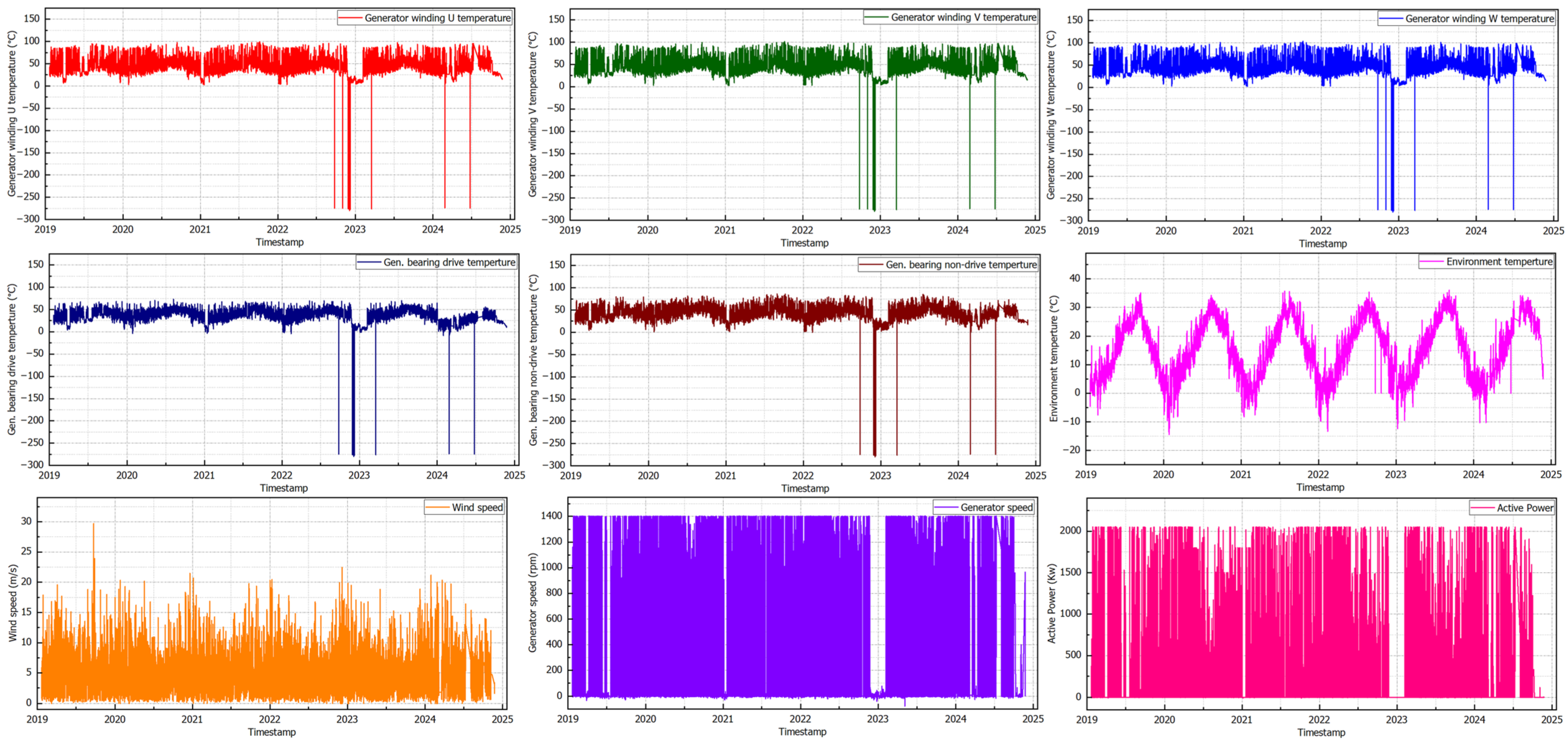
Figure 2 presents an overview of the SCADA channels selected as inputs to the generator RUL model for one representative 2 MW DFIG unit over the whole analysis period (2019–2025). The three upper-left panels show the stator winding temperatures for phases U, V, and W. For most of the period, all three traces lie within a narrow band between roughly 80 and 130 °C, consistent with the nominal operating range discussed earlier. Slow drifts in the mean level follow the seasonal evolution of the ambient temperature. In contrast, short negative spikes down to physically impossible values (e.g., below −100 °C) are clearly visible and correspond to sensor dropouts or communication errors. These artefacts are later removed during the preprocessing stage. The relative alignment of the three phase temperatures over long intervals indicates balanced cooling. In contrast, occasional persistent phase offsets provide evidence of local hot spots or a cooling imbalance, which will be reflected in the degradation indicators. The upper-right panels display the drive-end and non-drive-end bearing temperatures, as well as the generator speed. Bearing temperatures remain primarily in the range 40–75 °C, with a pattern similar to the stator windings: gradual seasonal trends and a small number of sharp outliers. The similarity between drive-end and non-drive-end profiles suggests that, for most of the horizon, the bearing pair experiences comparable thermal loading; deviations between them mark periods where misalignment or lubrication issues may arise and are later treated as abnormal episodes. Generator speed alternates between zero (turbine stopped) and the variable-speed operating band, with extended zero-speed regions corresponding to long shutdowns, grid outages, maintenance, or curtailment periods. These intervals are essential for the RUL model because they represent calendar time during which thermal ageing is significantly reduced, and they must be distinguished from missing-data episodes.

The middle-left panel shows the environment (nacelle) temperature, which exhibits a clear annual cycle between approximately −10 °C and 35 °C. This signal provides the reference for computing temperature rises (winding and bearing temperature minus ambient) and for discriminating genuine thermal overloads from benign changes driven by weather. For example, a moderate increase in absolute winding temperature during a hot summer period can correspond to a similar or even lower temperature rise when referenced to ambient and thus should not be interpreted as accelerated ageing. The middle-right panel reports the nacelle wind speed, which spans from near 0 m/s to values exceeding the rated region. The density of points in the 7–15 m/s band reflects typical onshore wind conditions and is consistent with the frequent operation close to rated power shown in the bottom panel.

Finally, the bottom panel depicts the generator’s active power over the same horizon. The signal oscillates between 0 and 2 MW, forming dense horizontal bands at or near rated power during normal production and deep gaps during extended shutdowns or curtailment. Short, isolated drops to zero within otherwise continuous production indicate brief trips or start/stop events, which may coincide with the temperature spikes observed in the upper panels. From the RUL perspective, this active-power trace, together with wind speed and generator speed, defines the operating-condition context in which thermal behaviour should be interpreted: long periods of high power and high temperature represent intense lifetime consumption, whereas low-power or idle periods contribute little to ageing.

Overall, Figure 2 confirms that the chosen SCADA channels form a long, regular multivariate record at a uniform 10 min resolution, capturing seasonal variation, different operating regimes, and the gradual evolution of generator temperatures over several years. These characteristics make the dataset well-suited for the preprocessing, operating-condition filtering, thermal-indicator construction, and lifetime-usage modelling steps described in the subsequent sections.

2.2. Maintenance and Failure Events

In addition to continuous SCADA measurements, the wind farm operator maintains a computerised maintenance management system and an associated event/alarm log. For each turbine and component, the system records the time stamp, turbine identifier, affected component, short fault description, and the maintenance action performed. These records are crucial for interpreting the long-term temperature and operating histories of the generator and for defining abnormal operating episodes used in the RUL analysis.

For the 2 MW DFIG considered in this study, all entries related to the generator between 2020 and 2025 were extracted and manually screened. The entries were grouped into the following two categories:

• Type A—major interventions: events involving internal generator repair, rewind, or full replacement, typically associated with extended downtime and significant dismantling of the machine.
• Type B—operational or auxiliary faults: events such as breaker maloperation, sensor faults, or protection trips which are corrected by inspection, component replacement, or control parameter adjustment but do not constitute the end of life of the generator.

Although the SCADA database encompasses an entire turbine fleet, this study focuses on a representative 2 MW onshore DFIG unit (2019–2025) for which multi-point generator temperature measurements and an audited maintenance log are available. During the observation window, the generator experienced several Type B events but no catastrophic Type A end-of-life failure. Consequently, Type B events are treated as abnormal operating episodes rather than true end-of-life points, and the proposed method is validated using trajectory-quality criteria—namely smoothness, abnormal responsiveness, and long-term trend consistency—rather than absolute RUL error against a confirmed failure timestamp. Two representative Type B events, summarised in

Table 3. The generator fault and maintenance history were used in the study.

Observation Date	Component	Fault Description (Abridged)	Interpretation in This Work
5 June 2023	Generator	The stator breaker opened during production or did not close synchronously with the grid-side converter.	Operational fault: used to mark an abnormal episode and check RUL response
13 October 2023	Generator	The on/off sensor does not operate	Auxiliary sensor fault; used to mark an abnormal episode and check RUL response

, are explicitly analysed in the case study; SCADA records around these timestamps show abrupt shifts in operating conditions accompanied by transient deviations in generator temperature profiles.

Because no full generator replacement occurred during the analysed period, the generator’s designed lifetime is used to define a nominal reference RUL trajectory based on the turbine’s elapsed calendar age. The fault and maintenance events in Table 3 are not treated as failure times; instead, they serve the following two purposes in the RUL framework:

• They define windows of abnormal operation against which the responsiveness of the RUL trajectory is evaluated (the model should show an accelerated decrease in RUL when persistent abnormal thermal behaviour occurs).
• They provide additional qualitative validation that the temperature- and operation-based degradation indicators used in the model are consistent with known disturbances in generator operation.

In summary, the maintenance and event data complement the SCADA time series by providing semantic labels for specific periods (normal vs. abnormal vs. post-maintenance), enabling a more meaningful evaluation of the proposed RUL model without requiring an actual end-of-life failure within the observation horizon.

3. RUL Estimation Framework

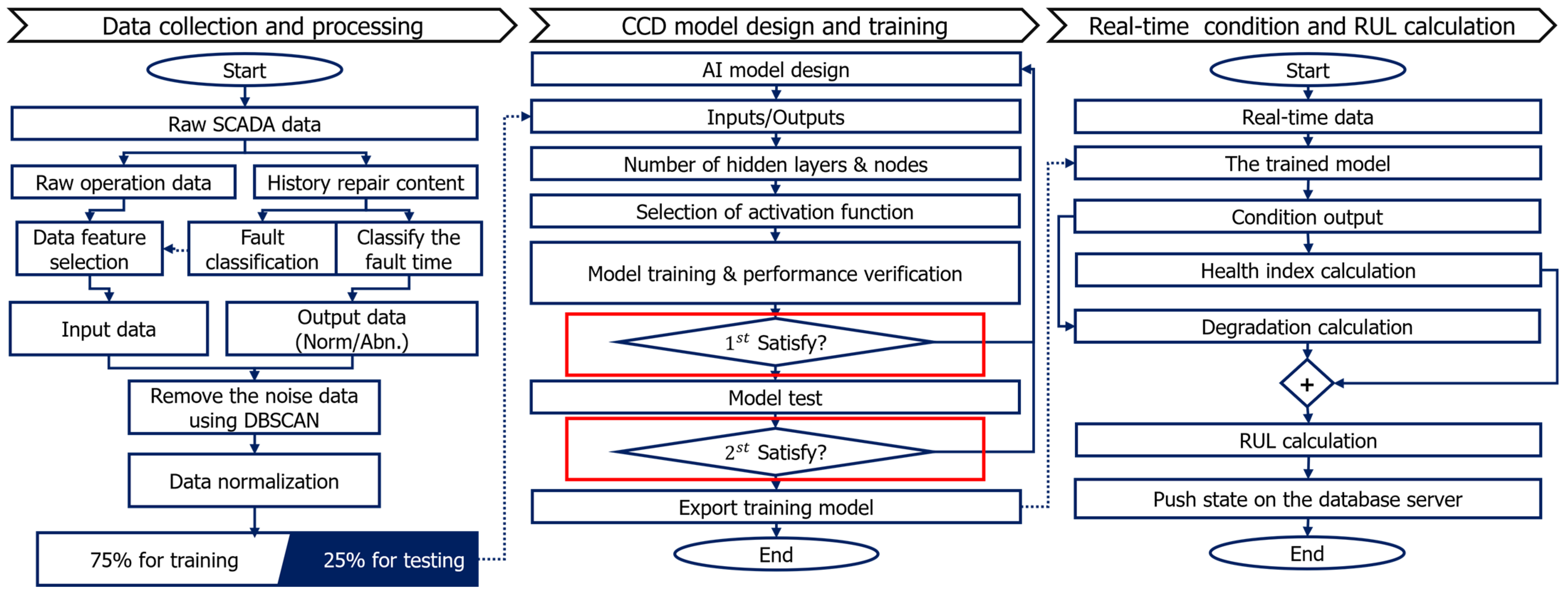
The proposed RUL framework follows a structured pipeline, summarised in Figure 3, which is explicitly designed to capture the thermal degradation of the most vulnerable generator components: the stator windings and the bearings. The process is divided into the following three main stages:

i.

Data collection and processing;

ii.

Condition-model design and offline training;

iii.

Real-time condition assessment and RUL calculation.

In essence, this structured pipeline transforms raw, noisy SCADA records into an intuitive maintenance signal by first filtering environmental variations, then quantifying the frequency (AOI) and severity (DegFactor) of thermal stress and finally mapping these daily indicators to a physically plausible, calendar-time RUL curve. In the data collection and processing stage (left part of Figure 3), raw SCADA data and repair histories are first extracted for the target turbine. The raw operation data consist of the 10 min averages of temperatures and operating variables described in Section 2.1, while the history-repair content contains time-stamped records of generator faults, repairs, and replacements. These two sources are aligned to define periods of normal operation and intervals related to specific fault events. A feature-selection step then identifies the subset of SCADA channels that carry the most information for generator condition and degradation (winding and bearing temperatures, ambient temperature, active power, speed, and basic status flags). Each 10 min record is labelled as “normal” or “abnormal” based on engineering rules and maintenance logs, yielding an input matrix and an associated output label vector (block “Input data/Output data (Norm./Abn.)”). To improve the robustness of the subsequent models, obvious noise points are removed using a density-based clustering (DBSCAN) based on outlier filter, which eliminates isolated samples in the feature space while preserving genuine high-load operating points. All remaining features are then normalised (for example, by min–max scaling or z-scores) so that different variables have comparable numerical ranges and the learning algorithm is not biased by units. Finally, the processed dataset is split into a training subset (75%) and a testing subset (25%); this split is fixed and used consistently in the following stages.

The condition-model design and training stage (centre of Figure 3) constructs a data-driven mapping from SCADA features to a condition output that summarises the generator’s instantaneous health state. Because of the selected inputs and desired outputs, an AI-based CCD model is specified: the model structure (type of regression/classifier), input–output definition, number of hidden layers and nodes, and activation functions are chosen to balance expressive power and computational cost. The model is then trained on the 75% training subset using an appropriate optimisation algorithm. During training, several performance indices (e.g., accuracy of normal/abnormal classification, false-alarm rate, and confusion matrix on known fault periods) are monitored. The first “Satisfy” decision in Figure 3 represents an internal check: if the indices do not meet predefined thresholds or if the model fails to detect known fault episodes, the architecture or hyperparameters are adjusted, and training is repeated. Once these internal criteria are satisfied, the model is frozen and evaluated on the 25% test subset; this second “Satisfy” decision ensures that the CCD model generalises to data not used in training. Only when both checks are passed is the trained model exported as the final condition-estimation block used in the online phase.

In the real-time condition and RUL calculation stage (right part of Figure 3), the exported CCD model is deployed at the SCADA or farm-server level. As real-time 10 min data from each turbine arrives, they pass through the same preprocessing chain used in training (feature construction, outlier filtering, and normalisation) to ensure consistency. The processed records are fed into the trained CCD model, which outputs, for each interval, an instantaneous condition indicator (e.g., normal/abnormal probability or condition score). These outputs are aggregated over a chosen time window (typically 14 days) to compute an AOI, which represents the fraction of points classified as abnormal during that day. The AOI is then combined with the thermal-degradation factor derived from generator temperature indicators (Section 3.2) to produce a health index (HI) expressed on a 0–100% scale. Conceptually, HI ≈ 100% corresponds to a generator operating close to its design envelope, whereas HI close to 0% indicates severe degradation or imminent failure.

Finally, the RUL calculation block converts the health index into a remaining lifetime expressed in calendar time. Using the generator’s design-lifetime curve as a reference, and the remaining useful life is obtained by subtracting the consumed portion from the nominal life. The resulting RUL value is updated every 10 min, smoothed over time to avoid spurious oscillations, and then written back to the database server along with the latest condition output. In this way, Figure 3 represents a closed loop: field SCADA data are continuously transformed into condition information, health indicators, and an interpretable RUL trajectory that operators can use for maintenance planning, alarm setting, and long-term asset-management decisions.

3.1. CCD-Based Condition Diagnosis Framework for the Generator

For the generator, the CCD model is implemented as a DNN classifier that maps multivariate SCADA measurements to a binary health label (Normal/Abnormal) for each 10 min record. The input vector $x_t$ at time index t is constructed from SCADA channels that are physically linked to generator thermal loading and operating state, such as stator-winding U/V/W temperatures, drive-end and non-drive-end bearing temperatures, generator frame temperature, generator speed, active power, nacelle wind speed, and ambient/nacelle air temperature. Historical alarm logs and maintenance records are used to define ground-truth bls $y_t\in \left\{1\right\}$: data belonging to clearly healthy operation (far from alarm thresholds, no relevant alarms, and no faults) are labelled $y_t=0$ (Normal), whereas data within predefined over-temperature regions, with persistent phase imbalance or close to trips, are labelled $y_t=1$ (Abnormal). Borderline periods around trips or sensor failures are discarded to avoid confusing the classifier.

To ensure reproducibility,

Table 4. Rule-based labelling protocol for CCD (Normal/Abnormal).

Signal Group	Condition for “Normal”	Condition for “Abnormal”
Winding temperature (U/V/W)	$\max \left(T_w\right)<140°\mathrm{C}$; phase imbalance $∆T<10°\mathrm{C}$	$T_w>140°\mathrm{C}$ (alarm) or $T_w>155°\mathrm{C}$ (trip) or persistent $∆T>10°\mathrm{C}$
Bearing temperature (DE/NDE)	$T_b$ within allowed operational range	$T_b\gtrsim 95°\mathrm{C}$ (alarm) or $T_b\gtrsim 105°\mathrm{C}$ (trip)
Environment temperature	Within allowed operational range	Extreme cold/heat causing derating or trip
Generator speed	Within normal band (0.7–1.1 pu)	Overspeed (alarm ~1.15 pu/trip ~1.25 pu)
State flags and alarms	Normal production	Fault, derated, or maintenance windows according to logs

summarises the rule set used to define Normal/Abnormal labels from SCADA alarms, temperature thresholds, and phase-imbalance criteria. In brief, a 10 min record is labelled Normal when all generator temperatures remain below alarm thresholds and phase imbalance remains within ${∆T}_{max}$; it is labelled Abnormal when any alarm/near-trip condition is present, when persistent phase imbalance exceeds ${∆T}_{max}$, or when a fault/derated state is reported in the maintenance log. Transitional windows (start-up/shutdown and a short buffer around alarm events) are excluded. Because abnormal events are rare in routine SCADA, the resulting dataset is typically class-imbalanced. We therefore use class-weighted training (or equivalent resampling) and select the decision threshold $\tau$ based on the ROC curve while prioritising recall for the Abnormal class to ensure robust fault detection.

Before training the DNN, the labelled dataset is carefully preprocessed. First, records with missing values, frozen signals, or obviously non-physical readings (e.g., negative power at high speed, temperature below sensor minimum) are removed. Next, short random spikes caused by communication noise are filtered using a DBSCAN in the normalised feature space: isolated points that do not belong to any dense cluster are treated as noise and eliminated. The remaining feature values are then standardised channel-wise to zero mean and unit variance:

$$z_{t,i}={\displaystyle \frac{x_{t,i}-{\mu }_i}{{\sigma }_i}}$$

(1)

where $x_{t,i}$ is the original value of feature $i$ at time $t$, and ${\mu }_i,{\sigma }_i$ are the mean and standard deviation computed over the training set. This scaling ensures that all inputs lie on a comparable numeric range and stabilises gradient-based optimisation. Finally, the cleaned dataset is split into training, validation and test subsets, typically using a 25% ratio while preserving the Normal/Abnormal class proportion in each subset (stratified split).

To ensure data quality before constructing the HI, an outlier removal process was performed using the DBSCAN algorithm. DBSCAN was employed to identify and eliminate abnormal SCADA measurements caused by sensor noise, communication interruptions, or transient operational disturbances. Unlike traditional threshold-based filtering, DBSCAN can effectively detect outliers in high-density operational datasets without requiring prior knowledge of cluster structures.

In this study, DBSCAN was applied to the selected generator operational variables within a five-dimensional feature space. The algorithm parameters were determined as follows:

• Neighbourhood radius (ε) = 0.3;
• Minimum number of points (MinPts) = 10.

The ε parameter was selected using the k-distance graph method, where the elbow point of the distance curve indicates the optimal neighbourhood radius for clustering. The MinPts parameter was chosen based on the common heuristic $MinPts\approx 2\times D$, where $D$ represents the dimensionality of the feature space.

By applying DBSCAN-based filtering, abnormal measurements were effectively removed prior to the HI construction stage, thereby improving the stability and reliability of the degradation trajectory used for RUL prediction.

The CCD network is designed as a fully connected feed-forward DNN. The input data were normalised using the StandardScaler method. The model consisted of three hidden layers, each containing 128 neurons, and the ReLU activation function was used in all hidden layers. The output layer employed a sigmoid activation function. The model was trained with a learning rate of 0.001 for 274 epochs. While static rules evaluate channels independently (e.g., alarming only when absolute temperature exceeds a hard limit), the DNN learns the multi-dimensional “healthy thermal envelope” conditioned on the operational state. This allows the model to detect anomalous cross-channel relationships—such as abnormally high temperatures occurring at low active power or in cold ambient conditions—long before univariate engineering thresholds are breached. Batch normalisation can be applied after each hidden layer to stabilise training, and dropout can be used to reduce overfitting. The output layer consists of a single neuron with a sigmoid activation that produces the estimated probability of abnormal operation:

$${\widehat{p}}_t=\sigma \left(h_{\theta }\left(z_t\right)\right)$$

(2)

where $z_t$ is the standardised input vector and $h_{\theta }\left(\cdot \right)$ denotes the composition of all hidden layers parameterised by $\theta$.

Model parameters $\theta$ are learned by minimising the binary cross-entropy loss over the training samples:

$$\mathcal{L}\left(\theta \right)=-{\displaystyle \frac{1}{N}}\sum _{t=1}^N\left[\hspace{0.17em}{y}_t\log {\widehat{p}}_t+\left(1-y_t\right)\log \left(1-{\widehat{p}}_t\right)\hspace{0.17em}\right]$$

(3)

Using mini-batch gradient descent with an adaptive optimizer (e.g., Adam). Early stopping on the validation loss is employed to prevent over-fitting; if the validation loss does not improve for a preset number of epochs, training is halted and the parameter set with the best validation performance is retained. Hyperparameters such as the number of layers/neurons, learning rate, batch size, and dropout rate are tuned by grid search or Bayesian optimisation, using the validation F1-score as the primary selection criterion.

Once trained, the CCD model is used to classify new SCADA records. For each 10 min record, the standardised feature vector $z_t$ is fed to the network to obtain ${\widehat{p}}_t$. A decision threshold $\tau$ is then applied to convert this probability into a discrete health label:

$${\mathrm{CCD}\_\mathrm{label}}_t=\left\{\begin{array}{cc}\mathrm{Abnormal}\left(1\right),& {\widehat{p}}_t\ge \tau \\ \mathrm{Normal}\left(0\right),& {\widehat{p}}_t<\tau \end{array}\right.$$

(4)

The threshold $\tau$ is selected based on the receiver-operating-characteristic (ROC) curve on the validation set, typically favouring high recall for Abnormal states while keeping the false-alarm rate acceptable for operation.

The trained CCD model is finally evaluated on the independent test subset using classification accuracy, precision, recall, F1-score, and confusion matrices to verify that abnormal thermal patterns are reliably separated from regular generator operation. In this way, the DNN-based CCD provides, for every 10 min SCADA record, a robust, data-driven Normal/Abnormal decision that is later aggregated and used as input to the subsequent degradation and RUL estimation stages.

3.2. Abnormal Operation Index and Degradation Factor Calculation

Once the CCD model described in Section 3.1 has been trained and deployed, its output is transformed into compact daily indicators that quantify how often the generator operates abnormally and the severity of the associated thermal loading. These indicators are the abnormal operation index (AOI) and the degradation factor, which together form the basis for the health index and RUL computation in the following sections.

3.2.1. Abnormal Operation Index

To obtain a daily measure of how frequently the generator leaves its learned standard envelope, a binary abnormality flag $z\left(k\right)$ is first defined using a decision threshold ${\tau }_{\mathrm{C}\mathrm{C}\mathrm{D}}$. The AOI(d) is defined as the fraction of intervals in day $d$ that are classified as abnormal:

$$AOI\left(d\right)={\displaystyle \frac{1}{\mid {\mathcal{K}}_d\mid }}\sum _{k\in {\mathcal{K}}_d}z\left(k\right)$$

(5)

By construction, $AOI\left(d\right)\in \left[0,1\right]$. Values close to zero indicate that the generator operated almost entirely within the normal region learned by the CCD, whereas values close to one indicate that most of the day was spent in abnormal states (e.g., persistent over-temperature, repeated trips or unusual combinations of load and speed). For interpretation and later evaluation, the following four qualitative bands are used:

• $0\le AOI\left(d\right)<0.10$: very healthy/stable operation;
• $0.10\le AOI\left(d\right)<0.35$: slight deviation, monitoring recommended;
• $0.35\le AOI\left(d\right)\le 0.60$: significant deviation from normal envelope;
• $AOI\left(d\right)>0.60$: highly abnormal operation.

In the RUL framework, AOI(d) acts as a frequency-type indicator: it describes how often abnormal episodes occur within each day but does not by itself encode how thermally severe those episodes are. The degradation factor provides this complementary information.

3.2.2. Degradation Factor Based on Thermal Severity

While the AOI quantifies the frequency of abnormal thermal behaviour, an additional indicator is required to describe the severity of operating conditions that may contribute to accelerated lifetime consumption. For this purpose, a degradation factor is introduced based on SCADA measurements.

For wind turbine generators, operational stress is mainly associated with electrical loading and mechanical operating conditions. In this study, the following two representative SCADA variables are used: the converter current and the generator rotational speed. These quantities reflect the electrical and mechanical operating regimes of the generator and therefore provide useful indicators of deviations from the turbine’s normal operating envelope.

For each day $d$, all SCADA records corresponding to normal power production are collected, and the daily mean values of the converter current and rotational speed are calculated as follows:

$${\bar{x}}_{cur}(d)={\displaystyle \frac{1}{N}}\sum _{i=1}^N{x}_{cur,i}(d)$$

(6)

$${\bar{x}}_{spd}(d)={\displaystyle \frac{1}{N}}\sum _{i=1}^N{x}_{spd,i}(d)$$

(7)

where $N$ is the number of valid SCADA samples during day $d$.

These daily mean values are then compared with reference operating levels representing the centre of the turbine’s typical operating envelope. The deviation of the observed operating conditions from these reference values is used to quantify the severity of operational departure from normal behaviour. The degradation factor for day $d$ is defined as follows:

$$DegFactor(d)=0.625{\displaystyle \frac{\mid {\bar{x}}_{cur}\left(d\right)-1170\mid }{1170}}+0.375{\displaystyle \frac{\mid {\bar{x}}_{spd}\left(d\right)-1260\mid }{1260}}$$

(8)

where 1170 A and 1260 rpm correspond to representative operating points of the studied turbine obtained from historical SCADA statistics. The weighting factors (0.625 and 0.375) reflect the relatively stronger influence of electrical loading compared with rotational speed in determining generator operational severity.

The numerical reference values used in Equation (8) (1170 A, 1300 A, 1260 rpm, and 560 rpm) are not universal constants of the proposed model. Instead, they are empirical parameters obtained from statistical analysis of the long-term SCADA dataset of the studied turbine. Specifically, the values 1170 A and 1260 rpm represent the typical average converter current and generator speed observed during normal power production, while 1300 A and 560 rpm correspond to the approximate operational ranges of these variables under healthy operating conditions.

These parameters therefore define the reference operating envelope of the specific turbine rather than fixed model constants. When the proposed framework is applied to other wind turbine types or wind farms, the same formulation can be retained by replacing these values with turbine-specific references derived from the corresponding SCADA statistics or from rated electrical and mechanical parameters. In this way, the degradation-factor formulation remains general and adaptable across different turbine models and operating conditions.

It is important to note that the DegFactor is not intended to represent a direct physical model of insulation thermal ageing. Instead, it serves as an operational deviation indicator derived from SCADA observations. Persistent deviations from the typical operating envelope—whether caused by abnormal loading conditions, control irregularities, or atypical operational regimes—may indicate operating states that deviate from the turbine’s normal behaviour.

Within the proposed framework, DegFactor is therefore used to describe the severity of operational deviation, while the AOI captures the frequency of abnormal thermal behaviour. The interaction of these two indicators is then incorporated into the lifetime-consumption formulation that determines the evolution of the RUL trajectory. In this way, the framework captures both the occurrence and the severity of abnormal operation, rather than relying on a single indicator.

3.2.3. Joint Use of AOI and Degradation Factor

AOI(d) and $\mathrm{D}\mathrm{e}\mathrm{g}\mathrm{F}\mathrm{a}\mathrm{c}\mathrm{t}\mathrm{o}\mathrm{r}\left(d\right)$ are designed to be used together, not in isolation. Conceptually, each day $d$ can be represented as a point in a two-dimensional plane whose axes are:

• Horizontal axis: how often the generator leaves its learned normal envelope (AOI(d));
• Vertical axis: how thermally severe the operation is during that day ($\mathrm{D}\mathrm{e}\mathrm{g}\mathrm{F}\mathrm{a}\mathrm{c}\mathrm{t}\mathrm{o}\mathrm{r}\left(d\right)$).

Days with both low AOI and low $\mathrm{D}\mathrm{e}\mathrm{g}\mathrm{F}\mathrm{a}\mathrm{c}\mathrm{t}\mathrm{o}\mathrm{r}$ correspond to benign operation and should consume lifetime at (or below) the nominal rate. In contrast, days with high AOI and high $\mathrm{D}\mathrm{e}\mathrm{g}\mathrm{F}\mathrm{a}\mathrm{c}\mathrm{t}\mathrm{o}\mathrm{r}$ indicate frequent and severe departures from normal behaviour and should be associated with accelerated lifetime consumption. The combined effect of these two quantities is captured through a scalar health index (HI) and a lifetime-usage factor, which together govern the evolution of the RUL trajectory.

To obtain a compact daily health measure, AOI(d) and $\mathrm{D}\mathrm{e}\mathrm{g}\mathrm{F}\mathrm{a}\mathrm{c}\mathrm{t}\mathrm{o}\mathrm{r}\left(d\right)$ are first combined into a dimensionless product that reflects both frequency and severity of abnormal operation. For numerical robustness, the degradation factor is saturated to a maximum value, ${\mathrm{D}\mathrm{e}\mathrm{g}\mathrm{F}\mathrm{a}\mathrm{c}\mathrm{t}\mathrm{o}\mathrm{r}}_{\mathrm{m}\mathrm{a}\mathrm{x}}$ (e.g., 1.5), so that isolated extreme outliers do not dominate the health estimate. The Health Index in day $d$ is then defined as follows:

$$HI\left(d\right)=100\left[\hspace{0.17em}1-AOI\left(d\right)\times \hspace{0.17em}\widetilde{\mathrm{D}\mathrm{e}\mathrm{g}\mathrm{F}\mathrm{a}\mathrm{c}\mathrm{t}\mathrm{o}\mathrm{r}}\left(d\right)\hspace{0.17em}\right]$$

(9)

where $\widetilde{\mathrm{D}\mathrm{e}\mathrm{g}\mathrm{F}\mathrm{a}\mathrm{c}\mathrm{t}\mathrm{o}\mathrm{r}}\left(d\right)=\min \left\{\mathrm{D}\mathrm{e}\mathrm{g}\mathrm{F}\mathrm{a}\mathrm{c}\mathrm{t}\mathrm{o}\mathrm{r}\left(d\right),\hspace{0.17em}{\mathrm{D}\mathrm{e}\mathrm{g}\mathrm{F}\mathrm{a}\mathrm{c}\mathrm{t}\mathrm{o}\mathrm{r}}_{\mathrm{m}\mathrm{a}\mathrm{x}}\right\}$.

By construction, $HI\left(d\right)\in \left[0,100\right]\mathrm{\%}$, where $HI\left(d\right)\approx 100\mathrm{\%}$ corresponds to nearly ideal operation (low AOI and low thermal severity) and $HI\left(d\right)\approx 0\mathrm{\%}$ corresponds to a highly degraded state with frequent and severe abnormalities. In practice, the following four qualitative bands are used to interpret daily health:

• $HI\left(d\right)\gtrsim 90\mathrm{\%}$: very healthy operation, life consumption close to nominal;
• $70\mathrm{\%}\lesssim HI\left(d\right)<90\mathrm{\%}$: early degradation, enhanced monitoring recommended;
• $40\mathrm{\%}\lesssim HI\left(d\right)<70\mathrm{\%}$: significant degradation, mid-term maintenance planning required;
• $HI\left(d\right)<40\mathrm{\%}$: high-risk regime, inspection, derating, or intervention should be considered.

This classification is not hard-coded into the RUL computation but provides a physically meaningful interpretation of the combined AOI and $\mathrm{D}\mathrm{e}\mathrm{g}\mathrm{F}\mathrm{a}\mathrm{c}\mathrm{t}\mathrm{o}\mathrm{r}$ information.

To connect the daily health state to lifetime consumption, a lifetime-usage factor (opentor $\left(d\right)$) is defined that scales the nominal daily consumption of the generator’s design lifetime. Let ${\lambda }_{\mathrm{nom}}$ denote the nominal fraction of life consumed per day under design operating conditions (derived from the 20-year design lifetime). Under perfect, fully healthy conditions, the generator would consume life at a rate ${\lambda }_{\mathrm{nom}}$. When AOI(d) and $\mathrm{D}\mathrm{e}\mathrm{g}\mathrm{F}\mathrm{a}\mathrm{c}\mathrm{t}\mathrm{o}\mathrm{r}\left(d\right)$ depart from their nominal values, the usage factor is increased in proportion to the combined abnormality level. A formulation is shown:

$$U\left(d\right)={\lambda }_{\mathrm{nom}}\left[\hspace{0.17em}1+\alpha \hspace{0.17em}AOI\left(d\right)\hspace{0.17em}\widetilde{\mathrm{D}\mathrm{e}\mathrm{g}\mathrm{F}\mathrm{a}\mathrm{c}\mathrm{t}\mathrm{o}\mathrm{r}}\left(d\right)\hspace{0.17em}\right]$$

(10)

The coefficient $\alpha$ in Equation (10) represents a calibration parameter that links the combined abnormality indicators to the accelerated consumption of the generator lifetime. In this study, the coefficient was empirically set to $\alpha$ based on calibration using the historical SCADA dataset of the studied turbine. The calibration procedure aimed to ensure that the resulting RUL trajectory satisfies two practical requirements. First, under healthy operating conditions where both $AOI\left(d\right)$ and $DegFactor\left(d\right)$ remain low, the lifetime consumption rate should follow closely the nominal design-life trend corresponding to the 20-year generator lifetime. Second, during sustained abnormal thermal operation, the model should produce a noticeably steeper decline in the RUL trajectory, reflecting accelerated degradation. The value $\alpha =0.35$ was selected as the smallest coefficient that allowed the model to clearly respond to abnormal operating episodes while preserving a physically plausible long-term RUL evolution. Although this coefficient is empirically calibrated for the studied turbine dataset, the proposed framework allows the parameter to be re-calibrated for other turbine types or wind farms depending on their operational characteristics. It does not correspond to a universal physical constant but rather acts as a system-level empirical coefficient that regulates how strongly abnormal operating conditions influence the daily life-usage rate. Specifically, the term $AOI\left(d\right)\times DegFactor\left(d\right)$ reflects the frequency and severity of abnormal thermal behaviour observed from SCADA measurements, while α converts this abnormality level into additional lifetime depletion beyond the nominal design rate.

When the generator operates under normal conditions, the abnormality term approaches zero and the lifetime consumption follows approximately the nominal design-life trajectory. In contrast, during periods of abnormal thermal operation, the value of $AOI\left(d\right)\times DegFactor\left(d\right)$ increases and the coefficient α amplifies the corresponding life consumption, leading to a steeper decline of the RUL trajectory. Because the available field dataset does not contain a complete run-to-failure record, $\alpha$ is empirically calibrated so that the resulting RUL trajectory remains consistent with the nominal lifetime trend during healthy operation while remaining sensitive to sustained abnormal thermal behaviour. Consequently, $\alpha$ should be interpreted as a turbine-specific calibration parameter whose value may vary depending on turbine type, operating conditions, and the SCADA dataset used.

Thus, AOI(d) and $\mathrm{D}\mathrm{e}\mathrm{g}\mathrm{F}\mathrm{a}\mathrm{c}\mathrm{t}\mathrm{o}\mathrm{r}\left(d\right)$ influence RUL in the following two complementary ways:

• Through HI(d), which offers an intuitive, operator-friendly view of the daily health status on a 0–100% scale, directly aligned with thermal and operational behaviour;
• Through $u\left(d\right)$, which mathematically converts the combined abnormality level into an incremental consumption of design lifetime in the RUL model.

In the subsequent sections, the cumulative sum of $u\left(d\right)$ overtime is compared against the generator’s nominal lifetime to construct a smooth, monotonically decreasing RUL trajectory. Days with low AOI and low $\mathrm{D}\mathrm{e}\mathrm{g}\mathrm{F}\mathrm{a}\mathrm{c}\mathrm{t}\mathrm{o}\mathrm{r}$ follow the design line closely, whereas clusters of high-AOI, high-severity days create local accelerations in lifetime usage and visibly sharper drops in the RUL curve. In this way, the joint use of AOI and the degradation factor ensures that the estimated RUL is both sensitive to abnormal thermal operation and consistent with long-term design-life expectations.

3.3. Lifetime-Consumption Mapping and RUL Trajectory Construction

For each 10 min SCADA record, the CCD model described in Section 3.1 outputs a label Normal or Abnormal. Over one calendar day $d$, these labels are aggregated into the abnormal operation index $AOI\left(d\right)$ defined as the proportion of abnormal samples on that day. In parallel, the degradation factor $DegFactor\left(d\right)$ (Section 3.2.2) quantifies how strongly the average current and speed deviate from their nominal values, i.e., how thermally severe the electrical loading is during that day. Together, $AOI\left(d\right)$ and $DegFactor\left(d\right)$ describe how often and how hard the generator is stressed on day $d$.

To obtain a long-term view of how much of the design life has been used, these daily usage factors are accumulated into an effective consumed lifetime. Let $\mathsf{\Delta }t$ denote one day expressed in the chosen lifetime unit (months). The cumulative consumption from the beginning of the observation period $d_0$ to a generic day $D$ is then defined as follows:

$$C(D)=\sum _{d=d_0}^{D}u\left(d\right)\hspace{0.17em}\mathsf{\Delta }t$$

(11)

Here, $C\left(D\right)$ is measured in “equivalent months at nominal loading”: if the generator operated exactly at nominal and conditions, $u\left(d\right)=1$ for all $d$ and $C\left(D\right)$ would increase linearly with calendar time. When abnormal operation occurs, larger values of $u\left(d\right)$ make $C\left(D\right)$ grow faster, directly reflecting the extra lifetime consumed by thermal stress.

The estimated remaining useful life at day $D$ is obtained by subtracting this effective consumption from the design lifetime $L_{\mathrm{des}}$ (20 years, expressed in months):

$$RU{L}_{\mathrm{est}}\left(D\right)=L_{\mathrm{des}}-C\left(D\right)$$

(12)

Because $AOI\left(d\right)$ and $DegFactor\left(d\right)$ are evaluated day by day, the raw RUL sequence can exhibit minor, jagged variations. To obtain a trajectory that reflects the slow nature of insulation ageing, a light temporal smoothing is applied using a moving average over a window of 14 days. This preserves the long-term trend and the response to multi-week abnormal episodes while filtering out day-to-day noise. The smoothed RUL trajectory is used in the results section for comparison with the nominal design line and for maintenance interpretation.

Because the inputs are calculated day by day, the raw RUL sequence can show minor, jagged variations. To obtain a trajectory that reflects the slow nature of insulation ageing, a light smoothing step is applied using a moving average window of 14 days. The proposed 14 days trailing moving-average scheme preserves online applicability; it introduces a trade-off between trajectory smoothness and immediate responsiveness to abrupt short-duration events. Therefore, the present framework is more suitable for long-term SCADA-based prognostic monitoring than for high-speed transient fault detection. Capturing extremely rapid degradation events may require additional event-level diagnostic modules with higher temporal resolution. This preserves the long-term trend and the response to multi-week abnormal episodes, while filtering out day-to-day noise. The smoothed RUL curve is the one used in the results and evaluation sections.

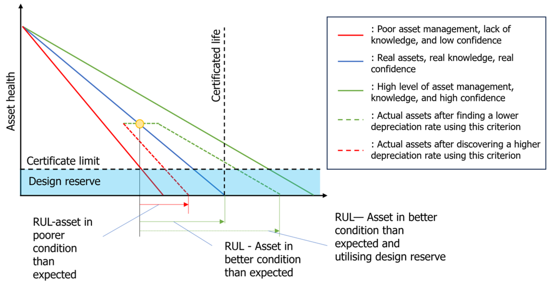
Figure 4 illustrates how the proposed lifetime-consumption mapping behaves under different operating histories. The horizontal axis represents calendar time from commissioning to the end-of-life horizon, and the vertical axis represents the remaining design lifetime. The blue solid line is the nominal design RUL. It decreases linearly from the initial lifetime to zero at the design end-of-life. The blue-shaded band below zero corresponds to the design reserve region, where the generator continues to operate beyond its nominal lifetime. The green solid line shows a case where the daily indices $u\left(d\right)$ remain small. In this case, the cumulative consumption $C\left(D\right)$ grows more slowly than calendar time, so the estimated RUL curve lies above the design line and reaches zero later. This corresponds to benign long-term usage in which some design margin remains at the nominal end-of-life. The red solid line represents a harsher scenario with frequent abnormal days. $C\left(D\right)$ accumulates quickly, and the RUL drops more steeply, crossing the zero-lifetime axis earlier than the design line. The yellow marker indicates the current evaluation date; the vertical distance from this point to the horizontal axis gives the predicted remaining lifetime at that date.

The green dashed line depicts a mixed case: the generator initially operates mildly (RUL above the blue line), then enters a prolonged abnormal phase. As a result, the slope of the RUL curve becomes steeper and eventually converges towards the design-reserve region. This lifetime-consumption and trajectory-construction step converts SCADA-derived abnormality measures into an interpretable curve of remaining calendar time. This curve directly supports maintenance planning by indicating how quickly the generator is degrading during real field operating conditions.

4. Operational Validation of the Proposed RUL Trajectory

4.1. The RUL Prediction Performance

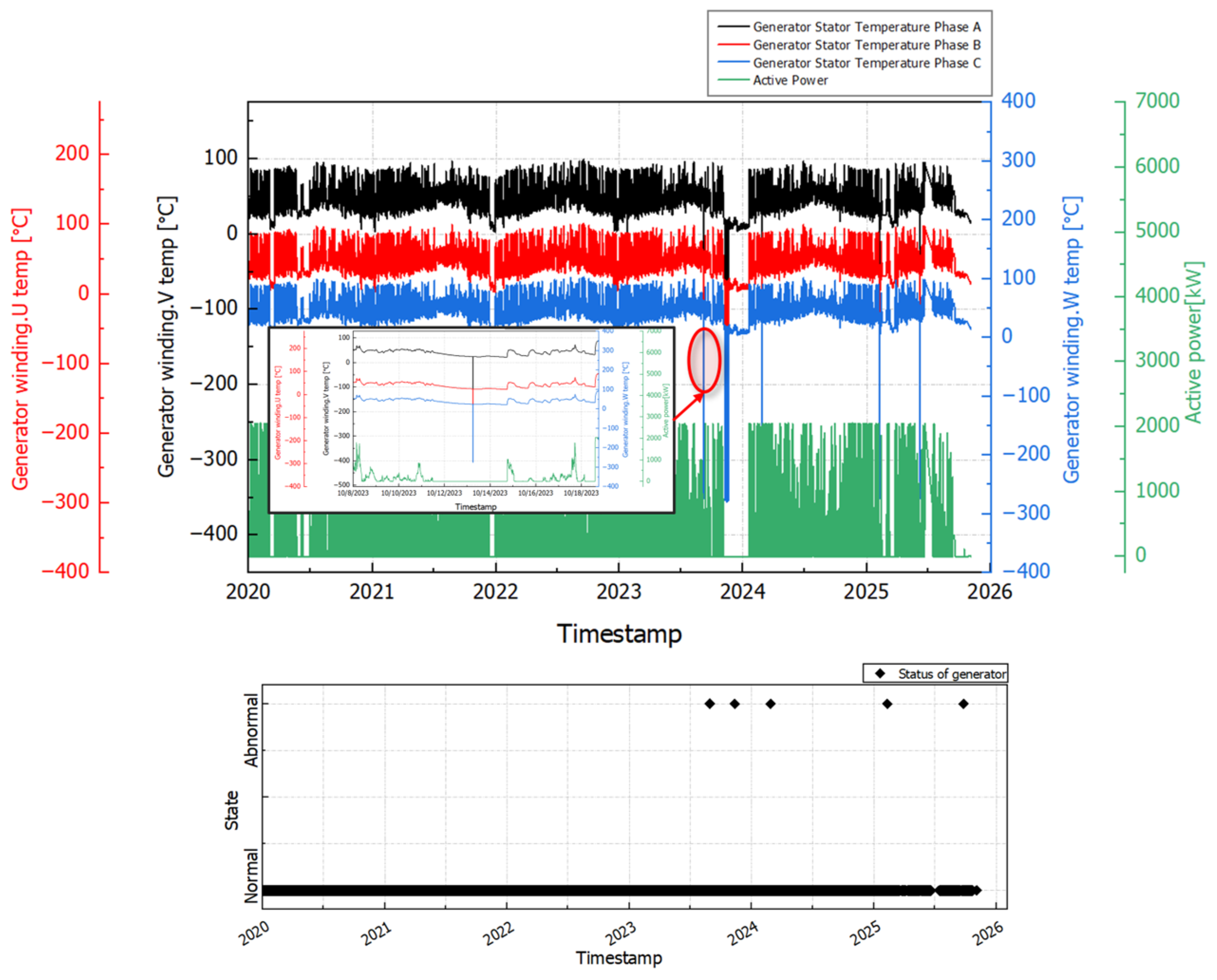
Figure 5 illustrates the long-term evolution of the generator stator winding temperatures in phases A, B, and C together with active power from 2020 to 2025, while the panel below it shows the corresponding binary status (“Normal/Abnormal”) supplied by the CCD model. Over almost the entire period, the three winding temperatures form a compact, nearly parallel bundle whose slow drift mainly reflects seasonal changes in ambient temperature and loading. The active power signal follows the expected production pattern with periods of high output and low output, but without sustained overloads. In the status plot, the overwhelming majority of days are classified as “Normal”; only a small number of short segments in late 2023 and early 2024 are labelled “Abnormal”. These abnormal segments coincide with clearly visible deviations in one or more winding temperatures and power and with a few isolated sensor artefacts that were removed in preprocessing. This confirms that, from a thermal perspective, the generator has been operated close to its design envelope, with only a limited number of genuinely abnormal operating episodes that can contribute to accelerated ageing.

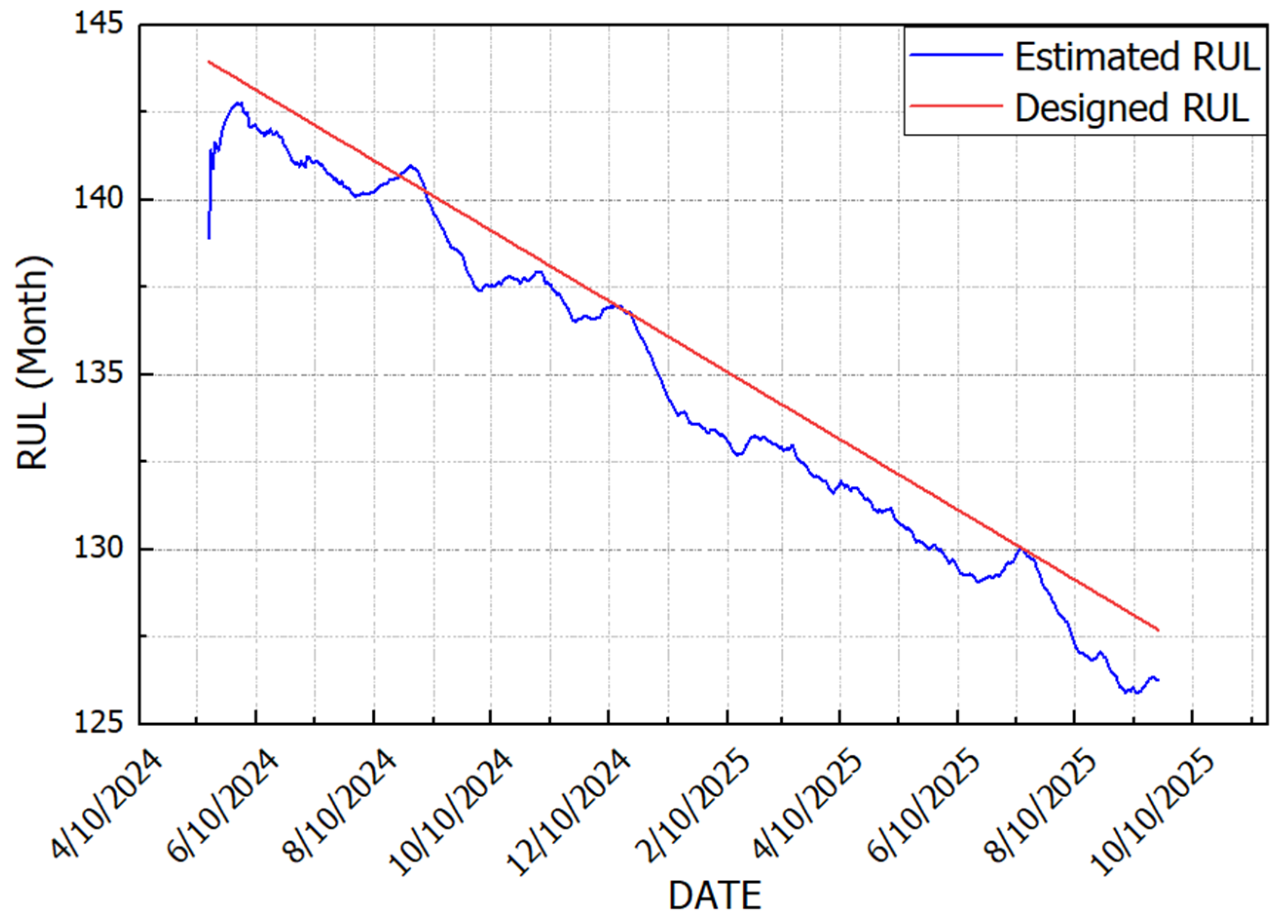
Figure 6 presents the resulting RUL trajectory for the generator over the evaluation horizon from mid-2024 to late 2025. The blue curve shows the estimated RUL obtained from the proposed lifetime-usage model. The red straight line indicates a design-life baseline under purely nominal loading, i.e., the remaining time to end-of-life assuming that the generator consumes its lifetime at a constant rate and that no abnormal operating events occur. In this work, the design life is set to 20 years (240 months), consistent with the typical wind turbine design lifetime used in wind farm asset planning. The baseline is plotted as a linear decrease because, under the constant-consumption assumption, the remaining life can be expressed as a linear function of elapsed calendar time (one month of operation consumes one month of lifetime under nominal conditions). This baseline does not represent a physics-of-failure model; instead, it serves as a reference to visualise additional lifetime consumption induced by historical and ongoing thermal usage.

At the beginning of the horizon, the estimated RUL starts slightly below the baseline (≈138–140 months versus ≈143–144 months), indicating that the accumulated thermal usage prior to June 2024 has already consumed an additional portion of the design life relative to nominal ageing. Over time, the blue curve decreases almost monotonically and remains consistently below the red line, as expected from the lifetime-consumption formulation. During long intervals where the CCD model reports normal operation and the AOI remains close to zero, the estimated RUL trajectory runs nearly parallel to the baseline, implying that the generator is ageing close to the nominal rate and no artificial penalty is introduced. In contrast, during abnormal episodes identified by elevated AOI, the slope of the blue curve increases, reflecting accelerated lifetime consumption under higher thermal/operational severity.

In contrast, around the dates where Figure 4 shows the slope of the blue RUL curve becomes visibly steeper than the red design line. These local accelerations correspond to windows where the abnormal operation index $AOI\left(d\right)$ and the degradation factor are elevated, causing the lifetime-usage factor $U\left(j\right)$ to increase and leading to larger incremental consumption in the RUL update. After the abnormal period ends and the generator returns to normal thermal behaviour, the slope gradually reverts to a value comparable to the design slope, so the RUL curve “re-joins” the design line without recovering above it. This behaviour demonstrates that the model is capable of selectively accelerating life consumption only when abnormal thermal stress is detected, while preserving a stable baseline when conditions are healthy.

4.2. The Evaluation Metrics and Validation Results

To verify that the proposed SCADA-driven framework yields a decision-ready and physically plausible RUL trajectory for wind turbine generators, the model is validated using three complementary evaluation criteria. Because the objective of this work is not only to produce numerically reasonable RUL values but also to generate a stable and interpretable trajectory for maintenance planning, the evaluation emphasises:

• Trajectory smoothness;
• Responsiveness to abnormal operation;
• Long-term linearity/consistency of RUL decay.

In field applications, SCADA measurements contain operational variability and sensor noise that can introduce artificial fluctuations in estimated health indicators. If these fluctuations propagate into RUL, the resulting trajectory may oscillate and become difficult to interpret, which reduces its usefulness for maintenance decision-making. Therefore, the first metric evaluates whether the proposed framework produces a smooth and stable RUL evolution without excessive short-term oscillations. Smoothness and near-monotonicity of the RUL curve, let $RU{L}_t$ [month] denote the estimated remaining useful life at day $t$. The day-to-day RUL change is defined as

$$\mathsf{\Delta }RU{L}_t=RU{L}_{t+1}-RU{L}_t$$

(13)

For a generator with a designed lifetime $L_{\mathrm{design}}$, we set a tolerance corresponding to approximately $0.1\mathrm{\%}$ of $L_{\mathrm{design}}$. In this study, this leads to a threshold of $\mathsf{\Delta }RU{L}_{\mathrm{th}}=0.24$ months. A day is classified as stable if the RUL variation does not exceed this tolerance:

$$\mid \mathsf{\Delta }RU{L}_t\mid \le \mathsf{\Delta }RU{L}_{\mathrm{th}}$$

(14)

Let $N_{\mathrm{stable}}$ denote the number of days that satisfy (15) and $N_{\mathrm{change}}$ the total number of days in the evaluation window. The smoothness ratio is then defined as

$${\eta }_{\mathrm{smooth}}={\displaystyle \frac{N_{\mathrm{stable}}}{N_{\mathrm{change}}}}\times 100\left[\mathrm{\%}\right]$$

(15)

Using the measured RUL trajectory, we obtain $N_{\mathrm{stable}}=486$ days and $N_{\mathrm{change}}=495$ days, thus:

$${\eta }_{\mathrm{smooth}}={\displaystyle \frac{486}{495}}\times 100\left[\mathrm{\%}\right]=98.182\left[\mathrm{\%}\right]$$

Using the proposed smoothing and monotonicity enforcement procedure in the RUL construction stage, the model achieves a smoothness of approximately 98.2%. It should be noted that this value represents an empirical ratio specific to the evaluated time window. Given the stochastic volatility of field SCADA data, it serves as a practical indicator of trajectory stability rather than a strict deterministic bound. Nevertheless, this high ratio indicates that only a very small fraction of the trajectory exhibits any upward fluctuations.

The idea of using an anomaly ratio as a driver for condition assessment is consistent with recent health-indicator designs for wind turbines, where the proportion or density of SCADA points classified as anomalous is aggregated into a scalar health index and used to support maintenance decisions [20]. Qiu et al., for example, proposed a robust wind-turbine component health status indicator built from anomaly detection on SCADA data and showed that the indicator reacts sensitively to abnormal operating regimes while remaining stable in healthy periods. In the present work, the abnormal-responsiveness metric plays a similar role at the RUL level: instead of directly visualising a health index, we require that the RUL trajectory systematically consumes more lifetime on days where AOI indicates thermally severe operation [21]. Responsiveness to abnormal operation (AOI-based criterion), abnormal operating behaviour is quantified by the AOI. For each day $d$, DBSCAN is applied to z-score normalised features; records labelled as noise are treated as abnormal SADA points. If $N_{\mathrm{outlier}}\left(d\right)$ and $N_{\mathrm{total}}\left(d\right)$ denote respectively the number of abcriteriaints and the total number of points that day, days with $AOI\left(d\right)\ge 0.40,$ are selected as abnormal-scenario 14 days. For each such day, we check whether the model reacts by consuming additional lifetime, i.e., whether the next-day RUL satisfies:

$$RU{L}_{d+1}<RU{L}_d$$

(16)

The model is said to “respond” to the anomaly on day $d$. Let $N_{\mathrm{abn}}$ denote the number of abnormal-scenario days and $N_{\mathrm{resp}}$ the number of those days for which (17) is satisfied. The abnormal-response ratio is then:

$${\eta }_{\mathrm{resp}}={\displaystyle \frac{N_{\mathrm{resp}}}{N_{\mathrm{abn}}}}\times 100\left[\mathrm{\%}\right]$$

(17)

From the results provided, there are $N_{\mathrm{abn}}=126$ abnormal days and for all of them $RU{L}_{d+1}<RU{L}_d$, so $N_{\mathrm{resp}}=126$. Hence:

$${\eta }_{\mathrm{resp}}={\displaystyle \frac{126}{126}}\times 100\left[\mathrm{\%}\right]=100\left[\mathrm{\%}\right]$$

(18)

The acceptance criterion was ${\eta }_{\mathrm{resp}}\ge 80\mathrm{\%}$. Achieving 100% means that every high-AOI day is followed by a decrease in RUL, showing that the model is fully sensitive to abnormal thermal usage. When AOI is low, the RUL curve follows the designed slope; when AOI spikes, the slope becomes steeper, as desired.

In parallel, AOI is combined with the degradation factor into a health index expressed in percent:

$$HI\left(j\right)=100\times \left(1-AOI\left(j\right)\cdot \mathrm{DegFactor}\left(j\right)\right)$$

(19)

Values close to 100% indicate near-new condition, while low values indicate severe degradation. For the studied generator, HI stays mostly in the 90–100% band, dropping below 70% only during a few abnormal periods, which is consistent with the limited number of high-AOI days and with the RUL accelerations observed.

In long-term linearity of the RUL trajectory method, a third requirement is that, over long horizons, the RUL trajectory should follow a nearly linear declining trend, reflecting gradual consumption of the designed lifetime. Beyond point-wise accuracy, several works have highlighted that a useful health indicator or RUL signal should exhibit a clear, nearly monotonic trend with time or degradation level. Monotonicity and trendability metrics have therefore been proposed to quantify how well a prognostic indicator follows a smooth degradation path. Our use of the coefficient of determination, also known as R-squared, between the estimated RUL and a linear design-lifetime trend follows this philosophy: a high $R^2$ value indicates that the predicted RUL trajectory behaves like a physically plausible, almost linear consumption of lifetime, whereas a low $R^2$ would reveal excessive curvature or oscillations that are difficult to reconcile with the generator’s design assumptions [22]. Abnormal operating behaviour is quantified by the abnormal operation index (AOI). For each day $d$, DBSCAN is applied to z-score-normalised SCADA features, and records labelled as noise are treated as abnormal points. If $N_{ab}\left(d\right)$ and $N_{tot}\left(d\right)$ denote the numbers of abnormal points and total points on day $d$, respectively, AOI is defined as in Equation (13). By construction, $0\le AOI\left(d\right)\le 1$, where larger values indicate more frequent abnormal operation during that day.

It is important to note that the life-consumption factor in Equation (7) is directly driven by the abnormality term. Therefore, a faster RUL decrease during high-AOI periods is mathematically expected and should not be interpreted as an independent validation of physical degradation. In this study, the purpose of the AOI-based responsiveness check is narrower: it is used to verify that the temporal smoothing applied to the daily RUL sequence does not mask or erase the degradation-related signal during abnormal thermal episodes. Days with $AOI\left(d\right)>0.30$ are selected as abnormal-scenario days. For each such day, the following condition is checked:

$$RUL(d+1)<RUL\left(d\right)$$

(20)

If this condition is satisfied, the trajectory is considered to preserve the abnormal-operation signal on that day. Let $N_{high}$ denote the number of abnormal-scenario days and $N_{resp}$ the number of days for which the above condition is satisfied. The AOI-based responsiveness ratio is then defined as in Equation (15).

From the results, all identified high-AOI days satisfy this condition, yielding a responsiveness ratio of 100%. This result indicates that the constructed and smoothed RUL trajectory preserves the accelerated life-consumption tendency during abnormal operating periods. However, this should be understood only as a numerical consistency check of signal preservation, not as an independent proof that the predicted RUL matches the true physical degradation process. These accuracy–type metrics are in line with prognostics evaluation practice, where point-wise errors between predicted and reference RUL and their statistics over time are widely used to quantify prediction quality. Saxena and Goebel introduced such error-based metrics as a core part of a general framework for evaluating prognostic algorithms, emphasising both bias and dispersion of RUL estimates. To quantify this, a simple linear regression is performed between RUL and elapsed time. Let $x_t$ denote the number of days since the start of the evaluation period for day $t$:

$$x_t=\left(Dat{e}_t-Dat{e}_{\mathrm{start}}\right)\hspace{0.17em}\left[\mathrm{day}\right]$$

(21)

A straight line is fitted to the pair $\left(x_t,RU{L}_t\right)$ using the affine model:

$$RU{L}_t=[a.\hspace{0.17em}{x}_t+b]$$

(22)

where $a$ [month/day] is the average RUL slope and $b$ [month] the intercept. For the generator case, the identified coefficients are

$$a=-0.041\mathrm{month}/\mathrm{day};b=140.411\mathrm{month}$$

which implies an average loss of about 0.041 month of RUL per calendar day.

The quality of this linear fit is measured using the coefficient of determination $R^2$:

$$SSR=\sum _t({RUL}_t-{\widehat{RUL}}_t{)}^2$$

(23)

be the sum of squared residuals between the observed RUL and the fitted line ${\widehat{RUL}}_t$, and:

$$SST=\sum _t({RUL}_t-\overline{RUL}{)}^2$$

(24)

the total sum of squares, where $\overline{RUL}$ is the mean RUL over the evaluation period. The coefficient of determination is defined as

$$R^2=1-{\displaystyle \frac{SSR}{SST}}$$

(25)

According to the reported values $SSR=3.548$ and $SST=239.100$, we obtain:

$$R^2=1-{\displaystyle \frac{3.548}{239.100}}\approx 0.985$$

The fitted trend yields $R^2=0.985$, indicating that the proposed framework produces a near-linear long-term RUL decay. This supports the intended behaviour of the lifetime-consumption mapping: the trajectory is dominated by a consistent ageing trend while still allowing local accelerations during abnormal episodes. Importantly, here $R^2$ is used only as a long-term trend consistency indicator, not as a primary accuracy metric for RUL prediction, thereby aligning with the practical objective of generating a reliable and interpretable RUL trajectory for maintenance planning.

Overall, the proposed framework satisfies three key requirements for field deployment: it generates an RUL trajectory that is highly smooth (98.2%), fully responsive to abnormal operation (100%), and consistent in its long-term decay trend ($R^2=0.985$). These results demonstrate that SCADA temperature–operation data can be transformed into a stable and decision-oriented generator RUL curve, supporting continuous condition assessment and proactive maintenance scheduling without additional sensing hardware. It should be noted that the studied generator did not experience a catastrophic Type A failure or full replacement during the observation period. Therefore, a true physical end-of-life timestamp is not available, and the proposed RUL trajectory cannot be interpreted as an absolute failure-time prediction. Instead, the estimated RUL should be understood as an effective lifetime-consumption indicator derived from SCADA-observed thermal and operational stress, intended to support maintenance planning under real field-data constraints.

5. Discussion and Conclusions

This study proposes a field-based RUL modelling framework for wind turbine generators using multi-year SCADA temperature and operational data, with the goal of producing a decision-ready and physically plausible RUL trajectory for maintenance planning. In contrast to conventional SCADA-based condition monitoring that relies largely on threshold alarms or qualitative trend inspection, the proposed approach transforms thermal usage and abnormal operation patterns into cumulative lifetime consumption and a stable calendar-time RUL curve. The following discussion interprets the validation outcomes, clarifies the practical implications, and summarises the main conclusions and future directions.

A key outcome of this work is that the model satisfies three fundamental requirements for SCADA-driven prognostics in real wind farm environments: trajectory smoothness, responsiveness to abnormal operation, and long-term consistency. First, the high smoothness score indicates that the constructed RUL trajectory is robust against short-term fluctuations introduced by SCADA noise and operating variability. This property is essential for deployment because oscillatory or frequently increasing RUL estimates tend to reduce operator trust and may lead to indecisive maintenance actions. By enforcing a stable and physically meaningful evolution during the RUL construction stage, the framework aligns the output with the irreversible nature of ageing in generator insulation systems and bearing-related thermal stress, thereby improving interpretability in day-to-day monitoring.

Second, the full responsiveness to abnormal operational episodes demonstrates that the framework is not merely producing a uniformly decreasing curve; instead, it dynamically reflects accelerated lifetime consumption when operating severity increases. In practical terms, this behaviour bridges the gap between “alarm-based monitoring” and “lifetime-aware prognosis”: abnormal thermal or operational episodes are mapped to a higher consumption rate and become visible as discernible changes in the RUL decay rate. This is critical for maintenance planning, because it provides an interpretable indication that degradation is accelerating under specific field conditions, allowing operators to prioritise inspection, adjust operating strategies, or prepare maintenance resources earlier than would be possible with threshold alarms alone.

Third, the near-linear long-term decay trend of the estimated RUL confirms that the lifetime-consumption mapping produces a coherent global trajectory over extended horizons. Importantly, this trend-consistency perspective should not be interpreted as the primary measure of prediction accuracy; instead, it verifies that the resulting RUL curve is structurally consistent with cumulative ageing behaviour while still allowing local accelerations during abnormal periods. This addresses the standard limitation of relying heavily on correlation-based metrics for RUL assessment, which may indicate trend similarity without guaranteeing a trajectory that is usable for maintenance decisions. In this study, the evaluation is therefore intentionally oriented toward trajectory quality and operational relevance.

From an application standpoint, the framework offers a practical advantage: it uses SCADA-only signals that are already available in most wind farms, thereby avoiding the cost and complexity of installing additional condition-monitoring sensors. This feature is significant for large fleets where retrofitting vibration or acoustic systems is economically challenging. Moreover, the generator-focused scope of the study addresses an area that is often less explored than gearbox or bearing prognostics, even though generator failures can drive significant downtime and repair costs. As a result, the proposed approach provides a scalable pathway to enhance predictive maintenance capabilities using existing infrastructure.

Despite these strengths, several limitations should be acknowledged. First, the studied generator did not experience a catastrophic Type A failure or a complete replacement during the observation period. As a result, a true run-to-failure ground truth is unavailable, and the predicted RUL trajectory should be interpreted as an effective lifetime-consumption indicator rather than an absolute end-of-life prediction. The present validation therefore focuses on trajectory quality and operational interpretability rather than direct failure-time prediction error. Broader evaluation across multiple wind farms, turbine ratings, generator designs, and climates will be necessary to further establish the general applicability of the framework. Second, the current framework primarily captures degradation through thermal and operational severity information. While thermal loading is strongly linked to generator ageing, additional indicators—such as electrical imbalance features, converter-related stress proxies, or condition-monitoring signals, when available—could further improve sensitivity to early-stage faults and strengthen fault-mode discrimination. Third, uncertainty is not explicitly quantified in the current trajectory; incorporating confidence bounds or probabilistic RUL outputs would be valuable for risk-aware decision-making, especially when planning maintenance under uncertain operating and weather conditions. Future research will focus on conducting comparative evaluations with representative RUL prediction approaches, including stochastic degradation models such as Wiener process-based methods and statistical time-series forecasting models such as ARIMA. These methods will be implemented using the same SCADA dataset and evaluated using consistent performance metrics in order to further analyse the advantages and limitations of the proposed HI-based RUL estimation framework.

In conclusion, this work demonstrates that multi-point generator temperature and operational SCADA data can be transformed into a stable, responsive, and long-horizon RUL trajectory suitable for practical maintenance planning. The proposed framework enables generator-focused RUL prognosis using SCADA-only data, explicitly links abnormal operation to accelerated lifetime consumption, and validates trajectory quality using complementary criteria that reflect real operational needs rather than relying solely on regression-style goodness-of-fit metrics. Future work will focus on expanding field validation, integrating additional degradation indicators, and incorporating uncertainty quantification to improve reliability and industrial applicability further.

References

1. Tchakoua, P.; Wamkeue, R.; Ouhrouche, M.; Slaoui-Hasnaoui, F.; Tameghe, T.A.; Ekemb, G. Wind Turbine Condition Monitoring: State-of-the-Art Review, New Trends, and Future Challenges. Energies 2014, 7, 2595–2630. [Google Scholar] [CrossRef]
2. Sikorska, J.Z.; Hodkiewicz, M.; Ma, L. Prognostic Modelling Options for Remaining Useful Life Estimation by Industry. Mech. Syst. Signal Process. 2011, 25, 1803–1836. [Google Scholar] [CrossRef]
3. Tautz-Weinert, J.; Watson, S.J. Using SCADA Data for Wind Turbine Condition Monitoring—A Review. IET Renew. Power Gener. 2017, 11, 382–394. [Google Scholar] [CrossRef]
4. Maldonado-Correa, J.; Martín-Martínez, S.; Artigao, E.; Gómez-Lázaro, E. Using SCADA Data for Wind Turbine Condition Monitoring: A Systematic Literature Review. Energies 2020, 13, 3132. [Google Scholar] [CrossRef]
5. Wang, Z.; Gao, P.; Chu, X. Remaining Useful Life Prediction of Wind Turbine Gearbox Bearings with Limited Samples Based on Prior Knowledge and PI-LSTM. Sustainability 2022, 14, 12094. [Google Scholar] [CrossRef]
6. Pandit, R.; Astolfi, D.; Hong, J.; Infield, D.; Santos, M. SCADA Data for Wind Turbine Data-Driven Condition/Performance Monitoring: A Review on State-of-Art, Challenges and Future Trends. Wind Eng. 2023, 47, 422–441. [Google Scholar] [CrossRef]
7. Cuesta, J.; Leturiondo, U.; Vidal, Y.; Pozo, F. A Review of Prognostics and Health Management Techniques in Wind Energy. Reliab. Eng. Syst. Saf. 2025, 260, 111004. [Google Scholar] [CrossRef]
8. Liu, X.; Du, J.; Ye, Z.S. A Condition Monitoring and Fault Isolation System for Wind Turbine Based on SCADA Data. IEEE Trans. Ind. Inform. 2022, 18, 986–995. [Google Scholar] [CrossRef]
9. Wang, S.; Vidal, Y.; Pozo, F. Recent Advances in Wind Turbine Condition Monitoring Using SCADA Data: A State-of-the-Art Review. Reliab. Eng. Syst. Saf. 2026, 267, 111838. [Google Scholar] [CrossRef]
10. Hu, Y.; Li, H.; Shi, P.; Chai, Z.; Wang, K.; Xie, X.; Chen, Z. A Prediction Method for the Real-Time Remaining Useful Life of Wind Turbine Bearings Based on the Wiener Process. Renew. Energy 2018, 127, 452–460. [Google Scholar] [CrossRef]
11. Rezamand, M.; Kordestani, M.; Orchard, M.E.; Carriveau, R.; Ting, D.S.K.; Saif, M. Improved Remaining Useful Life Estimation of Wind Turbine Drivetrain Bearings under Varying Operating Conditions. IEEE Trans. Ind. Inform. 2021, 17, 1742–1752. [Google Scholar] [CrossRef]
12. Carroll, J.; Koukoura, S.; Mcdonald, A.; Charalambous, A.; Weiss, S.; Mcarthur, S. Wind Turbine Gearbox Failure and Remaining Useful Life Prediction Using Machine Learning Techniques. Wind Energy 2019, 22, 360–375. [Google Scholar] [CrossRef]
13. Koukoura, S. Failure and Remaining Useful Life Prediction of Wind Turbine Gearboxes. In Proceedings of the Annual Conference of the PHM Society, Philadelphia, PA, USA, 24–27 September 2018. [Google Scholar]
14. Vieira, J.L.d.M.; Farias, F.C.; Ochoa, A.A.V.; de Menezes, F.D.; da Costa, A.C.A.; da Costa, J.Â.P.; de Novaes Pires Leite, G.; Vilela, O.d.C.; de Souza, M.G.G.; Michima, P.S.A. Remaining Useful Life Estimation Framework for the Main Bearing of Wind Turbines Operating in Real Time. Energies 2024, 17, 1430. [Google Scholar] [CrossRef]
15. Lan, X.; Liang, D.; Liu, W.; Wang, Y.; Han, Y.; Yu, Z. Remaining Useful Life Prediction of Wind Turbine Generator Bearings Based on Nonlinear Wiener Process. In Proceedings of the 2023 3rd Power System and Green Energy Conference, PSGEC 2023, Shanghai, China, 24–26 August 2023; Institute of Electrical and Electronics Engineers Inc.: New York, NY, USA, 2023; pp. 1124–1129. [Google Scholar]
16. Guo, P.; Infield, D.; Yang, X. Wind Turbine Generator Condition-Monitoring Using Temperature Trend Analysis. IEEE Trans. Sustain. Energy 2012, 3, 124–133. [Google Scholar] [CrossRef]
17. Peter, R.; Zappalá, D.; Schamboeck, V.; Watson, S.J. Wind Turbine Generator Prognostics Using Field SCADA Data. J. Phys. Conf. Ser. 2022, 2265, 032111. [Google Scholar] [CrossRef]
18. Wang, K.S.; Sharma, V.S.; Zhang, Z.Y. SCADA Data Based Condition Monitoring of Wind Turbines. Adv. Manuf. 2014, 2, 61–69. [Google Scholar] [CrossRef]
19. Baboli, P.T.; Babazadeh, D.; Raeiszadeh, A.; Horodyvskyy, S.; Koprek, I. Optimal Temperature-Based Condition Monitoring System for Wind Turbines. Infrastructures 2021, 6, 50. [Google Scholar] [CrossRef]
20. Deng, S.; Zhou, J. Prediction of Remaining Useful Life of Aero-Engines Based on CNN-LSTM-Attention. Int. J. Comput. Intell. Syst. 2024, 17, 232. [Google Scholar] [CrossRef]
21. Lázaro, R.; Melero, J.J.; Yürüşen, N.Y. A Robust Wind Turbine Component Health Status Indicator. Appl. Sci. 2024, 14, 7256. [Google Scholar] [CrossRef]
22. Saxena, A.; Celaya, J.; Saha, B.; Saha, S.; Goebel, K. Metrics for Offline Evaluation of Prognostic Performance. Int. J. Progn. Health Manag. 2010, 1, 4–23. [Google Scholar] [CrossRef]
Figure 1. External and cut-away view of the 2 MW DFIG.
Energies 19 01722 g001
Figure 2. Generator input data selection in the RUL model.
Energies 19 01722 g002
Figure 3. Process of the RUL model for the components of the wind turbine.
Energies 19 01722 g003
Figure 4. Concept of design lifetime consumption and generator RUL trajectories.
Energies 19 01722 g004
Figure 5. Long-term evolution of the generator with CCD-based normal/abnormal status.
Energies 19 01722 g005
Figure 6. Estimated generator RUL trajectory compared with the nominal design-life baseline.
Energies 19 01722 g006