A Stackelberg Game-Based Model of the Distribution Network Planning in Local Energy Communities

Abstract

The electrical characteristics of distribution networks (DNs) are drastically changing, which is mainly due to widespread adoption of small-scale distributed energy resources (DERs) by end-users. In these cases, conventional planning models may lead to overinvestment choices. This paper presents a planning model for utility companies that explicitly incorporates a model of end-users’ energy-related decisions, considering a neighborhood energy trading scheme (NETS). The model is formulated based on the Stackelberg game (SG) approach, which guarantees the optimality of the final solution for each user and the utility. The proposed mixed-integer second-order cone programming (MISOCP) problem finds the optimal investment plan for transformers, lines, distributed generators (DGs), and energy storage systems (ESSs) for the utility, considering the scenarios of end-users’ investments in rooftop photovoltaic (PV) and battery systems that maximize their benefits. Additionally, a dynamic network charge (NC) scheme is designed to rationalize the network use. Also, Benders decomposition (BD) is used to improve the convergence of the solution algorithm. The numerical studies on a real 23-bus low voltage (LV) network in Perth, Australia, using real-world data reveals that the proposed planning model offers the lowest total cost and the highest penetration of DERs in comparison with conventional models.

1. Introduction

Distribution network (DN) planning focuses on identifying efficient investment plans that ensure safe grid operation at a minimal cost. The performance of planning tools is largely affected by energy users’ characteristics. As end-users increasingly adopt small-scale distributed energy resources (DERs), utilities invest more in the DN to manage the transition towards a customer-centric energy system. In this context, this paper develops a planning framework that explicitly accounts for the interactions between utilities and end-users within a local energy community (LEC).

The integration of renewable energy technologies in DN planning has been extensively studied in the literature [1,2,3,4,5,6,7,8,9,10,11,12,13]. In [2], a planning method is proposed to incorporate the investment in both the centralized and distributed energy storage systems (ESSs). Similar coordinated DN planning studies are reported in [14,15,16,17]. Both temporary non-network solutions and conventional network solutions are incorporated into the risk-managed planning technique proposed in [4]. The modern renewable technologies and demand response (DR) programs are used in [3,5,6] to reinforce the DNA planning technique, based on the genetic algorithm presented in [7] for DER allocation in radial DNs. In [8], a scenario-based stochastic DER planning technique is used, which incorporates the decision regarding the investment in wind turbines, PVs, and ESSs. The sizing of DERs is planned in [9], using a data-driven algorithm to guarantee the convergence to the global optimal solution in DNs. A mixed-integer linear programming (MILP) model is presented in [10] to find the optimal investment plan, considering DERs, capacitor banks, voltage regulators, and conductor replacements. The application of distributed ESSs in alleviating the PV impacts on DNs is exploited in [11]. The concept of active DNs (ADNs) and formulation of optimization problems for them has been investigated in the recent literature [17,18,19]. In [19], a multi-stage stochastic planning model for ADNs is presented.

More recent studies have extended DN planning models by incorporating additional dimensions such as flexibility, resilience and reliability within DNs. A cooperative planning framework is proposed in [20] to enhance the resilience of ADNs under extreme events by coordinating the network assets with aggregated distributed resources and network reconfiguration capabilities. Also, recent works have investigated the coordinated planning of ESSs in ADNs, accounting for seasonal load variations and different operating scenarios [21,22]. Furthermore, coordinated planning models that jointly consider DERs and ESSs have been formulated to reduce the total investment and operating costs while improving voltage regulation and reducing emissions under stochastic conditions [23,24,25]. Also, coordinated transmission and distribution expansion planning frameworks have been investigated in [26]. A bilevel coordination planning model is proposed in [27], which utilizes an electrical distance-based partitioning method to optimize the placement and capacity of distributed photovoltaic (PV) and ESS. However, all the reviewed techniques in DN planning have been limited to cost minimization for the utility and investments in the DN and do not address the benefit maximization of users in LECs.

Some planning studies have considered ESS and DR as potential alternatives to conventional network reinforcements [28,29]. These models aim to integrate flexible resources into DN expansion planning to defer or reduce infrastructure investments. However, end-users’ investment and operational decisions are often represented in an aggregated or exogenous manner.

In [30], a bi-level framework is proposed to coordinate peer-to-peer energy trading with distribution network reconfiguration, enabling prosumers to exploit demand-side flexibility while allowing the distribution system operator to manage the network security and losses under multi-period AC power flow constraints. Similarly, ref. [31] developed a distributed community-based local energy market, using an ADMM-based coordination scheme to minimize individual prosumer costs while explicitly enforcing distribution network constraints and preserving privacy under uncertain renewable generation. Most existing works focus on operational coordination and short-term scheduling, rather than long-term planning with discrete investment variables. As a result, the explicit modeling of strategic interactions between utilities and end-users in DN planning problems remains limited.

Decision making for end-users has become an important trend in modern power systems [20,21,22]. Due to advances in communication technologies and new regulatory frameworks, in several cases, users can now trade energy with other users on a local energy platform, e.g., a neighborhood energy trading (NET) scheme, that enables the users to exchange excess local generation (e.g., from rooftop PV or stored energy in batteries) with other users connected to the network. Some literature presents approaches for the benefit maximization for end-users in LECs with a peer-to-peer market [20,22] or in DR programs [21], without considering the interests of the utility. This motivates the development of a planning platform that accounts for the impact of end-users’ investments in DERs on the optimal DN investment plan. This paper aims to provide a link between the planning techniques for the utility and the decision-making tools for the end-users by adopting a Stackelberg Game (SG) approach.

SG has been identified as an efficient approach to represent the problems with the leader–follower structure, including the DR programs [21,32] and energy management in microgrids [33] and smart grids [34]. However, these studies mainly focus on small-scale continuous programming models, where power quantities and prices are exchanged between the leader and the followers. The inclusion of integer variables, particularly investment decisions in planning studies, has rarely, if ever, been explored in the literature. This is mainly because introducing integer variables makes it challenging to prove the existence of a Stackelberg equilibrium (SE).

In this paper, we focus on developing a planning model that incorporates the end-users’ decisions in LECs. Also, a NETS is added to the model, which allows the end-users to exchange energy. The proposed model also provides a scheme for the selection of network charge (NC) levels for the participants in the NETS. To improve the convergence of the proposed solution strategy, the Benders decomposition (BD) is applied. The planning framework developed in this paper benefits the utilities by considering the end-users’ decision making in DN planning. In that sense, any deviation in end-users’ decisions can be treated as a source of uncertainty in the problem. The uncertainties of load demand, renewable generation, and the whole price are considered by scenario-based techniques [35].

The contributions of this work are summarized as follows:

(1)

The development of a planning procedure for the utility that explicitly represents users’ investment scenarios and guarantees the optimality of the solution for both the utility and end-users.

(2)

The modeling of the integrated planning problem based on the SG approach, represented as a mixed-integer second-order cone programming (MISOCP) problem. This work expands the application of SG in modern DNs.

(3)

The inclusion of NETS in DN planning and the definition of a procedure for the choice of NCs.

(4)

The adoption of BD for solving the proposed planning problem, which converts a MILP problem with a high number of integer variables into a linear programming (LP) problem. The decomposed problem exhibits considerably improved convergence.

This work differs from previous SG-based models by explicitly integrating utility’s DN planning with end-user investment decisions, including NETS design, NCs for planning insights and a decomposition-based solution for MISOCP problems. To the best of our knowledge, no existing study combines these elements within a unified planning framework.

Typically, studies applying BD assume a convex subproblem to guarantee convergence. In this work, the subproblem is nonconvex and includes integer variables. Bilinear nonconvexities are reformulated using auxiliary variables, and feasible integer solutions are generated iteratively. This combination of reformulation and selective enumeration effectively produces a convex subproblem at each iteration, enabling the decomposition-based approach to be applied reliably.

The specific NETS considered in the paper is described in Section 2. The planning and operation model of each end-user that participates in the NETS is presented in Section 3. The planning and operation model for the utility is formulated in Section 4. Section 5 explains the SG and the solution strategy. The case study is presented in Section 6, and Section 7 concludes the paper.

2. The Concept of Neighborhood Energy Trading

The NET in this paper is a scheme in which end-users in the same LV network can trade electrical energy with other participants. End-users equipped with DER facilities can sell the energy produced by their solar PV or storage systems to other end-users in their neighborhood via the NETS. In this paper, there are four types of firms involved in the NETS, as follows:

• Consumers: The end-users with no DER facilities. A consumer can only act as a buyer in the NETS.
• Prosumers: The end-users that own DERs and can trade energy with other participants in their neighborhood. A prosumer can act as either a seller or a buyer in the NETS, depending on the available state of charge of their battery, PV generation profile, load profile and profitability of the traded energy.
• NET operator: The agent responsible for determining the energy price and ensuring the balance between demand and supply. The NET operator sends the NC values to NET participants. It is important to note that the operator acts solely in the interest of the NET participants.
• Utility: The utility company is responsible for designing the NC levels and sending them to the NET operator. The NC represents the charge paid by NET participants for the use of the network. In practice, such charges are typically regulated and reflected in retail electricity prices. In this study, it is assumed that the utility sets the NC only to improve the efficient use of the network, rather than to maximize the profit, and that the NC values are therefore capped.

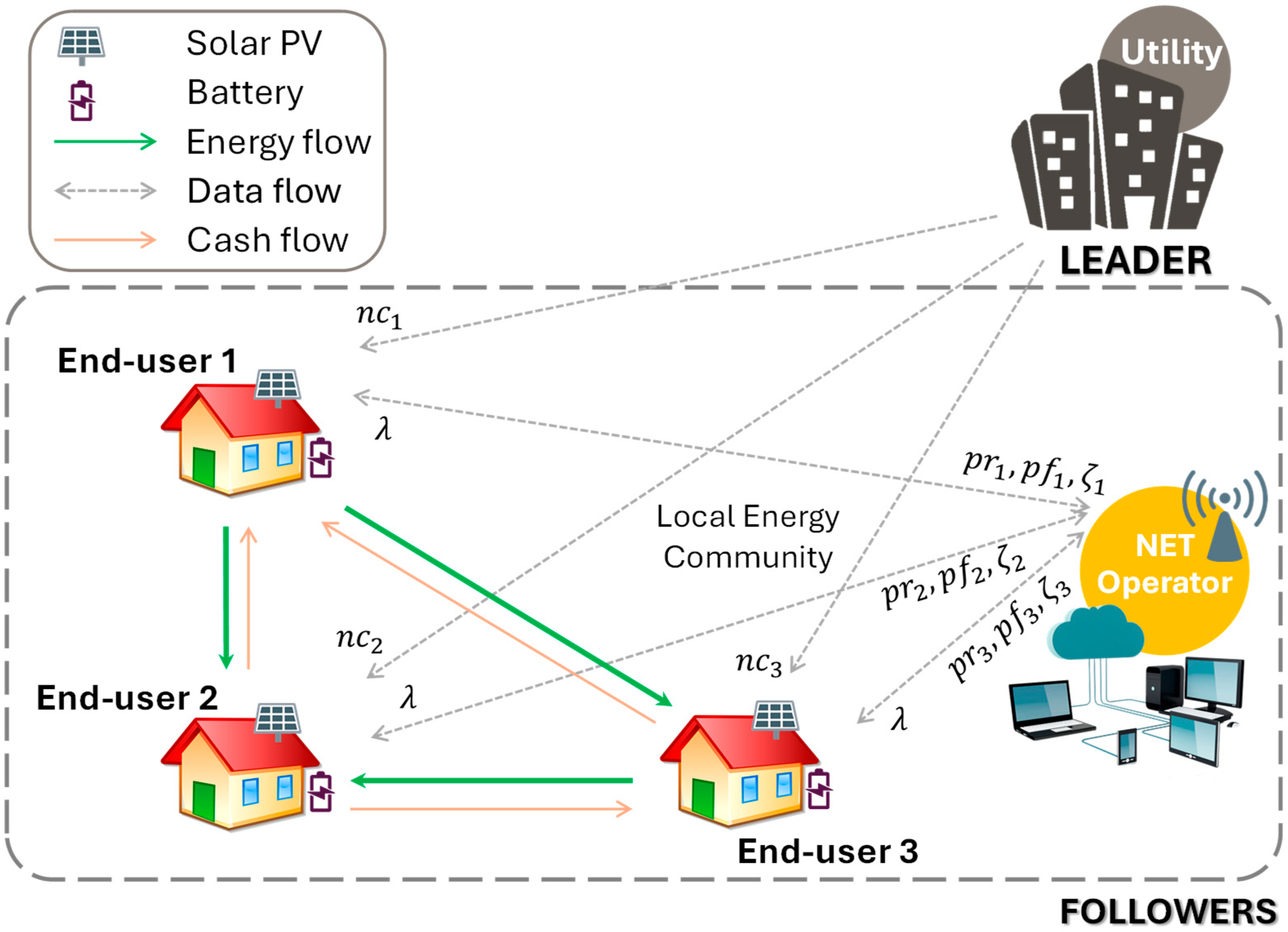
Figure 1 shows the structure of the proposed NETS. In this figure, some end-users act as sellers, while others act as buyers. The NET operator uses the operating schedules submitted by end-users to determine the energy price, denoted as $\mathsf{\lambda }$. The operating schedule includes energy purchased from the utility, energy exported to the grid under the feed-in tariff program and the energy traded within the NETS, denoted by $p{r}_i$, $p{f}_i$ and ${\mathsf{\zeta }}_i$ for the end-user at the $\mathrm{i}$-th bus. The operator is responsible for maintaining the demand–supply balance within the NETS and, if necessary, procuring additional energy from the utility, which offers less attractive prices than local trading. The utility sets the NC prices for NET participants, denoted by $n{c}_i$ where $\mathrm{i}$ represents the end-user at the $\mathrm{i}$-th bus. NCs are intended to promote efficient use of network infrastructure. End-users respond to the NC values set by the utility by adjusting their energy-related decisions to minimize their individual costs.

Given the NC values, the NET operator determines the energy price, ${\mathsf{\lambda }}_t$, based on the submitted operating schedules. The end-users then update their schedules and resubmit them to the NET operator. This iterative process continues until convergence is achieved between the operator and the end-users. Once the energy trades in the NETS are finalized, the operator forwards the operating schedules to the utility, which subsequently updates the NC values. Similar to the iterative interaction between the NET operator and end-users, the interaction between the operator and the utility continues until a consistent solution is reached. If a mismatch between demand and supply remains, the NET operator resolves it through transactions with the utility. In short, the NETS functions as a market mechanism in which an operator clears the local supply and demand and determines the energy price. The NET operator may be an independent agent whose role is to maximize the benefit of participating end-users.

The design of the proposed NETS resembles an SG, which models decision-making problems with a leader–follower structure wherein the leader will make the decisions first, and the followers respond accordingly. In this paper, the utility acts as the leader by setting the NC values, while the end-users act as followers who adjust their energy-related decisions in response, as shown in Figure 1. The proposed NC signals apply only to transactions within the NET framework and do not alter regulated electricity tariffs. The purpose of these signals is to reflect network impacts, rather than to recover costs or discriminate among users.

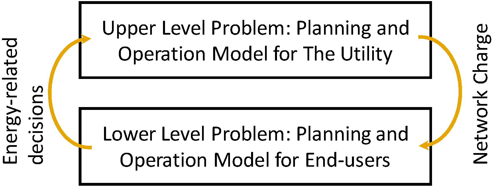
Using this bilevel Stackelberg framework, a new planning model is developed that incorporates both the investment and operational decisions of the utility (Section 4), and those of the end-users (Section 3), as shown in Figure 2. The complete bilevel SG formulation is presented in Section 5.

3. Operation of Neighborhood Energy Trading

The goal in the NET is the minimization of the total cost of electricity incurred by the LEC and to guarantee that participation in the NET is convenient for all the end-users without cross subsidization. In the considered scheme, this is achieved by solving a decision-making problem for the entire LEC that is decomposed into smaller subproblems using the Lagrangian decomposition technique. The solution to the decomposed dual problem provides the solution to the original problem.

The centralized planning and operation of end-users is formulated in (1)–(17):

$$\underset{\begin{array}{c}{x}_{\mathit{ij}}^{\mathrm{PV}}, x_{\mathit{ik}}^{\mathrm{B}}, {\mathit{pr}}_{\mathit{it}}, {\mathit{pf}}_{\mathit{it}}, {\zeta }_{\mathit{it}}, d_{\mathit{it\tau }}, {\pi }_{\mathit{it}}, {\alpha }_{\mathit{it}}^{\mathrm{B}}, {\mathit{SoC}}_{\mathit{it}}^{\mathrm{B}}, {\mathit{SoC}}_{i,\mathit{max}}^{\mathrm{B}},\\ {\mathit{SoC}}_{i,\min }^{\mathrm{B}}, {\mathit{pc}}_{i,\max }^{\mathrm{B}}, {\mathit{pd}}_{i,\max }^{\mathrm{B}}, {\mathit{pc}}_{\mathit{it}}^{\mathrm{B}}, {\mathit{pd}}_{\mathit{it}}^{\mathrm{B}}, {\mathit{BDC}}_i^{\mathrm{B}}\end{array}}{\min }J$$

(1)

$$J={\sum }_{i\in \mathsf{\Theta }}{J}_i$$

(2)

$$\begin{array}{c}{J}_i={\sum }_{t\in {\mathsf{\Theta }}^{\mathrm{t}}}{\mathrm{R}}_t{pr}_{it}-{\sum }_{t\in {\mathsf{\Theta }}^{\mathrm{t}}}{\mathrm{F}}_t{pf}_{it}+{\sum }_{t\in {\mathsf{\Theta }}^{\mathrm{t}}}{\mathrm{L}}_t{\zeta }_{it}+{\sum }_{t\in {\mathsf{\Theta }}^{\mathrm{t}}}{nc}_{it}{\pi }_{it}+\\ {\mathrm{D}\mathrm{F}}_i{\sum }_{t\in {\mathsf{\Theta }}^{\mathrm{D}\mathrm{R}\mathrm{F}},\tau \in {\mathsf{\Theta }}^{\mathrm{D}\mathrm{R}\mathrm{T}}}{d}_{it\tau }+{\sum }_{j\in {\mathsf{\Theta }}^{\mathrm{P}\mathrm{V}}}{\mathrm{C}\mathrm{P}\mathrm{V}}_j{x}_{ij}^{\mathrm{P}\mathrm{V}}+{\sum }_{k\in {\mathsf{\Theta }}^{\mathrm{B}\mathrm{T}}}{\mathrm{C}\mathrm{B}}_k{x}_{ik}^{\mathrm{B}}+{BDC}_i^{\mathrm{B}}\end{array}$$

(3)

subject to the constraints defined by (4)–(17), below.

In (1) and (2), $J$, $\mathrm{R}$, $\mathrm{F}$, $\mathrm{L}$, $nc$, $\mathrm{D}\mathrm{F}$, $\mathrm{C}\mathrm{P}\mathrm{V}$ and $\mathrm{C}\mathrm{B}$ denote the total cost function, retail price, feed-in tariff, energy price in the NETS, NC, disutility factor for the end-users due to shifting their scheduled load demand (which quantifies the cost borne by consumers as a result of deviating from their scheduled demand), the capital cost of PV and the capital cost of the battery, respectively. Also, $p{r}_{it}$, $p{f}_{it}$, ${\zeta }_{it}$ and ${\pi }_{it}$ represent the purchased energy from the utility, the injected energy to the grid under the feed-in tariff program, the exchanged energy in the NETS (with sign +/− indicating buying/selling), and the absolute value of exchanged energy in the NETS of user $i$ at time interval $t$, respectively. Also, $d_{it\tau }$, $BD{C}_i$, $x_{ij}^{\mathrm{P}\mathrm{V}}$ and $x_{ik}^{\mathrm{B}}$ are the shifted load from hour $t$ to hour $\tau$, the battery degradation cost, and the investment states of candidate PV unit $j$ and candidate battery $k$ of user $i$, respectively. ${\mathsf{\Theta }}^{\mathrm{D}\mathrm{R}\mathrm{T}}$ and ${\mathsf{\Theta }}^{\mathrm{D}\mathrm{R}\mathrm{F}}$ are the sets of time intervals to and from which the load demand can be shifted, respectively. The cost function in (2) includes the PV installation cost, battery installation cost, cost of energy purchased from the utility, cost of energy purchased in the NETS, negative cost associated with selling energy in the NETS, cost of NC, cost of DR and battery degradation cost.

The energy balance in the NETS is

$${\sum }_{i\in \mathsf{\Theta }}{\zeta }_{it}=0\forall t \in {\mathsf{\Theta }}^{\mathrm{t}}$$

(4)

where the total demand and supply are equal. Grid losses are not included in this equation, as the utility is responsible for covering the losses. The utility compensates for the cost of grid losses through the NC.

The detailed model of each user’s cost minimization problem is formulated as follows:

(1)

Battery operation constraints.

$${SoC}_{it}^{\mathrm{B}} \le \mathrm{M}{\sum }_{k\in {\mathsf{\Theta }}^{\mathrm{B}}}{x}_{ik}^{\mathrm{B}}$$

(5)

$$\left\{\begin{array}{c}{SoC}_{i,\mathrm{m}\mathrm{a}\mathrm{x}}^{\mathrm{B}}={\sum }_{k\in {\Theta }^B}{\overline{SoC}}_k{x}_{ik}^{\mathrm{B}}, {SoC}_{i,\mathrm{m}\mathrm{i}\mathrm{n}}^{\mathrm{B}}={\sum }_{k\in {\mathsf{\Theta }}^{\mathrm{B}}}{\underset{\_}{SoC}}_k{x}_{ik}^{\mathrm{B}}\\ {pc}_{i,\mathrm{m}\mathrm{a}\mathrm{x}}^{\mathrm{B}}={\sum }_{k\in {\mathsf{\Theta }}^{\mathrm{b}\mathrm{t}}}\overline{{\mathrm{p}\mathrm{c}}_k}{x}_{ik}^{\mathrm{B}}, {pd}_{i,\mathrm{m}\mathrm{a}\mathrm{x}}^{\mathrm{B}}={\sum }_{k\in {\mathsf{\Theta }}^{\mathrm{B}}}\overline{{\mathrm{p}\mathrm{d}}_k}{x}_{ik}^{\mathrm{B}}\end{array}\right.$$

(6)

$${SoC}_{i,\mathrm{m}\mathrm{i}\mathrm{n}}^{\mathrm{B}}\le {SoC}_{it}^{\mathrm{B}}\le {SoC}_{i,\mathrm{m}\mathrm{a}\mathrm{x}}^{\mathrm{B}}$$

(7)

$${pc}_{it}^{\mathrm{B}}\le {pc}_{i,\mathrm{m}\mathrm{a}\mathrm{x}}^{\mathrm{B}}, {pd}_{it}^{\mathrm{B}}\le {pd}_{i,\mathrm{m}\mathrm{a}\mathrm{x}}^{\mathrm{B}}$$

(8)

$${SoC}_{it}^{\mathrm{B}}={SoC}_{i,t-1}^{\mathrm{B}}+{\mathsf{\eta }}_c{pc}_{it}^{\mathrm{B}}-{\displaystyle \frac{1}{{\mathsf{\eta }}_d}}{pd}_{it}^{\mathrm{B}}$$

(9)

$${pc}_{it}^{\mathrm{B}}\le \mathrm{M}{\alpha }_{it}^{\mathrm{B}}, {pd}_{it}^{\mathrm{B}}\le \mathrm{M}\left(1-{\alpha }_{it}^{\mathrm{B}}\right)$$

(10)

$${BDC}_i^{\mathrm{B}}={\mathrm{B}\mathrm{D}}_i^{\mathrm{B}}{\sum }_{t\in {\mathsf{\Theta }}^{\mathrm{t}}}\left({pc}_{it}^{\mathrm{B}}+{pd}_{it}^{\mathrm{B}}\right)$$

(11)

$${\mathsf{\eta }}_c{\sum }_{t\in {\mathsf{\Theta }}^{\mathrm{t}}}{pc}_{it}^{\mathrm{B}}={\displaystyle \frac{1}{{\mathsf{\eta }}_d}}{\sum }_{t\in {\mathsf{\Theta }}^{\mathrm{t}}}{pd}_{it}^{\mathrm{B}}$$

(12)

The battery operation is modeled in (5)–(12). The state of charge ($SoC$) is set to zero in (5) when the battery is not available. The maximum and minimum SoC of the battery, as well as the maximum charging and discharging power, are defined in (6). The SoC of the battery is limited by (7). The charging and discharging power of the battery are defined in (8). The SoC of the battery is calculated in (9). The operating state of the battery is determined by an integer variable, i.e., ${\mathsf{\alpha }}_{it}^{\mathrm{B}}$, where zero denotes discharging and one denotes charging, as outlined in (10). In (11), the total cost of depreciation is presented. Finally, the net energy stored in the battery over a day is forced to be zero in (12).

(2)

NETS operation constraints.

$${\pi }_{it} \ge {\zeta }_{it}, {\pi }_{it} \ge -{\zeta }_{it}$$

(13)

The absolute value of the traded energy in the NETS in (13) is required to calculate the cash flow between the NET participants and the utility.

(3)

Demand response limits.

$${\sum }_{\tau \in {\mathsf{\Theta }}^{\mathrm{D}\mathrm{R}\mathrm{T}}}{d}_{it\tau } \le {\mathrm{d}}_{it}^{\mathrm{m}\mathrm{a}\mathrm{x}} \forall t \in {\mathsf{\Theta }}^{\mathrm{D}\mathrm{R}\mathrm{F}}$$

(14)

The amount of shifted demand which will be determined in the optimization is limited in (14).

(4)

Power balance constraints.

$$\left\{\begin{array}{c}{\mathrm{D}}_{it}-{\sum }_{j\in {\mathsf{\Theta }}^{\mathrm{P}\mathrm{V}}}{\mathrm{G}}_{jt}{x}_{ij}^{\mathrm{P}\mathrm{V}}+{pc}_{it}^{\mathrm{B}}-{pd}_{it}^{\mathrm{B}}+{\sum }_{\tau \in {\mathsf{\Theta }}^{\mathrm{D}\mathrm{R}\mathrm{F}}}{d}_{i\tau t}={pr}_{it}-{pf}_{it}+{\zeta }_{it} \forall t\in {\mathsf{\Theta }}^{\mathrm{D}\mathrm{R}\mathrm{T}}\\ {\mathrm{D}}_{it}-{\sum }_{j\in {\mathsf{\Theta }}^{\mathrm{P}\mathrm{V}}}{\mathrm{G}}_{jt}{x}_{ij}^{\mathrm{P}\mathrm{V}}+{pc}_{it}^{\mathrm{B}}-{pd}_{it}^{\mathrm{B}}-{\sum }_{\tau \in {\mathsf{\Theta }}^{\mathrm{D}\mathrm{R}\mathrm{T}}}{d}_{i\tau t}={pr}_{it}-{pf}_{it}+{\zeta }_{it} \forall t\in {\mathsf{\Theta }}^{\mathrm{D}\mathrm{R}\mathrm{F}}\\ {\mathrm{D}}_{it}-{\sum }_{j\in {\mathsf{\Theta }}^{\mathrm{P}\mathrm{V}}}{\mathrm{G}}_{jt}{x}_{ij}^{\mathrm{P}\mathrm{V}}+{pc}_{it}^{\mathrm{B}}-{pd}_{it}^{\mathrm{B}}={pr}_{it}-{pf}_{it}+{\zeta }_{it} \forall t\in {\mathsf{\Theta }}^{\mathrm{t}}-\left({\mathsf{\Theta }}^{\mathrm{D}\mathrm{R}\mathrm{F}}\cup {\mathsf{\Theta }}^{\mathrm{D}\mathrm{R}\mathrm{T}}\right)\end{array}\right.$$

(15)

The energy balance of each end-user is presented in (15) for the time slots in ${\mathsf{\Theta }}^{\mathrm{D}\mathrm{R}\mathrm{T}}$, ${\mathsf{\Theta }}^{\mathrm{D}\mathrm{R}\mathrm{F}}$, and other time slots.

(5)

Construction constraints.

$${\sum }_{j\in {\mathsf{\Theta }}^{\mathrm{P}\mathrm{V}}}{x}_{ij}^{\mathrm{P}\mathrm{V}}\le 1, {\sum }_{k\in {\mathsf{\Theta }}^{\mathrm{B}}}{x}_{ik}^{\mathrm{B}}\le 1$$

(16)

Constraint (16) limits the number of installed PV or battery units to a maximum of one unit per user.

By expanding (2) using (3), we get:

$$\begin{array}{c}J ={\sum }_{i\in \mathsf{\Theta },j\in {\mathsf{\Theta }}^{\mathrm{P}\mathrm{V}}}{\mathrm{C}\mathrm{P}\mathrm{V}}_j{x}_{ij}^{\mathrm{P}\mathrm{V}}+{\sum }_{i\in \mathsf{\Theta },k\in {\mathsf{\Theta }}^{\mathrm{B}}}{\mathrm{C}\mathrm{B}}_k{x}_{ik}^{\mathrm{B}}+{\sum }_{i\in \mathsf{\Theta }}{BDC}_i^{\mathrm{B}}+\\ {\sum }_{i\in \mathsf{\Theta },t\in {\mathsf{\Theta }}^{\mathrm{D}\mathrm{R}\mathrm{F}},\tau \in {\mathsf{\Theta }}^{\mathrm{D}\mathrm{R}\mathrm{T}}}{\mathrm{D}\mathrm{F}}_i{d}_{it\tau }+{\sum }_{i\in \mathsf{\Theta },t\in {\mathsf{\Theta }}^{\mathrm{t}}}\left({\mathrm{R}}_t{pr}_{it}-{\mathrm{F}}_t{pf}_{it}+{\mathrm{L}}_t{\zeta }_{it}+{nc}_{it}{\pi }_{it}\right)\end{array}$$

(17)

Combining (4) and (17), we obtain (18) as follows:

$$\begin{array}{c}J ={\sum }_{i\in \mathsf{\Theta },j\in {\mathsf{\Theta }}^{\mathrm{P}\mathrm{V}}}{\mathrm{C}\mathrm{P}\mathrm{V}}_j{x}_{ij}^{\mathrm{P}\mathrm{V}}+{\sum }_{i\in \mathsf{\Theta },k\in {\mathsf{\Theta }}^{\mathrm{B}}}{\mathrm{C}\mathrm{B}}_k{x}_{ik}^{\mathrm{B}}+{\sum }_{i\in \mathsf{\Theta }}{BDC}_i^{\mathrm{B}}+\\ {\sum }_{i\in \mathsf{\Theta },t\in {\mathsf{\Theta }}^{\mathrm{D}\mathrm{R}\mathrm{F}},\tau \in {\mathsf{\Theta }}^{\mathrm{D}\mathrm{R}\mathrm{T}}}{\mathrm{D}\mathrm{F}}_i{d}_{it\tau }+{\sum }_{i\in \mathsf{\Theta },t\in {\mathsf{\Theta }}^{\mathrm{t}}}\left({\mathrm{R}}_t{pr}_{it}-{\mathrm{F}}_t{pf}_{it}+{nc}_{it}{\pi }_{it}\right)\end{array}$$

(18)

According to (18), the dual problem is

$$\max \varphi \left(\overline{\lambda }\right), \overline{\lambda }\ge 0$$

(19)

$$\begin{array}{c}\varphi \left(\overline{\lambda }\right)=\min \{{\sum }_{i\in \mathsf{\Theta },j\in {\mathsf{\Theta }}^{\mathrm{P}\mathrm{V}}}{\mathrm{C}\mathrm{P}\mathrm{V}}_j{x}_{ij}^{\mathrm{P}\mathrm{V}}+{\sum }_{i\in \mathsf{\Theta },k\in {\mathsf{\Theta }}^{\mathrm{B}}}{\mathrm{C}\mathrm{B}}_k{x}_{ik}^{\mathrm{B}}+{\sum }_{i\in \mathsf{\Theta }}{BDC}_i^{\mathrm{B}}+\\ {\sum }_{i\in \mathsf{\Theta },t\in {\mathsf{\Theta }}^{\mathrm{D}\mathrm{R}\mathrm{F}},\tau \in {\mathsf{\Theta }}^{\mathrm{D}\mathrm{R}\mathrm{T}}}{\mathrm{D}\mathrm{F}}_i{d}_{it\tau }+{\sum }_{i\in \mathsf{\Theta },t\in {\mathsf{\Theta }}^{\mathrm{t}}}\left({\mathrm{R}}_t{pr}_{it}-{\mathrm{F}}_t{pf}_{it}+{nc}_{it}{\pi }_{it}\right)-{\sum }_{t\in {\mathsf{\Theta }}^{\mathrm{t}}}{\lambda }_t{\sum }_{i\in \mathsf{\Theta }}{\zeta }_{it}\}\end{array}$$

(20)

For the considered MILP problem, the duality gap is negligible, i.e., the mixed integer and the corresponding relaxed linear version have the same optimal value; therefore, the duality theorem implies that

$$\min J=\max \varphi \left(\overline{\lambda }\right)$$

(21)

Using the Lagrangian decomposition, for a given value of $\overline{\mathsf{\lambda }}={\overline{\mathsf{\lambda }}}_0$, we have

$$\begin{array}{c}\varphi \left({\overline{\lambda }}_0\right)=\min \{{\sum }_{i\in \mathsf{\Theta },j\in {\mathsf{\Theta }}^{\mathrm{P}\mathrm{V}}}{\mathrm{C}\mathrm{P}\mathrm{V}}_j{x}_{ij}^{\mathrm{P}\mathrm{V}}+{\sum }_{i\in \mathsf{\Theta },k\in {\mathsf{\Theta }}^{\mathrm{B}}}{\mathrm{C}\mathrm{B}}_k{x}_{ik}^{\mathrm{B}}+{\sum }_{i\in \mathsf{\Theta }}{BDC}_i^{\mathrm{B}}+\\ {\sum }_{i\in \mathsf{\Theta },t\in {\mathsf{\Theta }}^{\mathrm{D}\mathrm{R}\mathrm{F}},\tau \in {\mathsf{\Theta }}^{\mathrm{D}\mathrm{R}\mathrm{T}}}{\mathrm{D}\mathrm{F}}_i{d}_{it\tau }+{\sum }_{i\in \mathsf{\Theta },t\in {\mathsf{\Theta }}^{\mathrm{t}}}\left({\mathrm{R}}_t{pr}_{it}-{\mathrm{F}}_t{pf}_{it}-{\lambda }_{0t}{\zeta }_{it}+{nc}_{it}{\pi }_{it}\right)\}\end{array}$$

(22)

Considering (21), any feasible solution of the dual problem defined in (19)–(22) is a lower bound for the original problem defined in (1)–(16). Also, (22) can be decomposed as follows:

$$\varphi \left({\overline{\lambda }}_0\right)={\sum }_{i\in \mathsf{\Theta }}{\varphi }_i\left({\overline{\lambda }}_0\right)$$

(23)

$$\begin{array}{c}{\varphi }_i\left({\overline{\lambda }}_0\right)=\min \{{\sum }_{j\in {\mathsf{\Theta }}^{\mathrm{P}\mathrm{V}}}{\mathrm{C}\mathrm{P}\mathrm{V}}_j{x}_{ij}^{\mathrm{P}\mathrm{V}}+{\sum }_{k\in {\mathsf{\Theta }}^{\mathrm{B}}}{\mathrm{C}\mathrm{B}}_k{x}_{ik}^{\mathrm{B}}+{BDC}_i^{\mathrm{B}}+\\ {\mathrm{D}\mathrm{F}}_i{\sum }_{t\in {\mathsf{\Theta }}^{\mathrm{D}\mathrm{R}\mathrm{F}},\tau \in {\mathsf{\Theta }}^{\mathrm{D}\mathrm{R}\mathrm{T}}}{d}_{it\tau }+{\sum }_{t\in {\mathsf{\Theta }}^{\mathrm{t}}}\left({\mathrm{R}}_t{pr}_{it}-{\mathrm{F}}_t{pf}_{it}-{\lambda }_{0t}{\zeta }_{it}+{nc}_{it}{\pi }_{it}\right)\}\end{array}$$

(24)

Equations (23) and (24) render a decomposed structure of the original problem in (1)–(16). The resulting subproblems correspond to each end-user and can be solved in parallel to enhance computational speed. As such, the vector of Lagrangian multipliers, ${\overline{\lambda }}_0$, is updated iteratively by the NET operator until there is no significant change compared to the previous iteration.

Following the Lagrangian decomposition, the planning and operation problem of each end-user is formulated as (25)–(27)

$$\min J_i$$

(25)

$$\begin{array}{c}{J}_i={\sum }_{t\in {\mathsf{\Theta }}^{\mathrm{t}}}{\mathrm{R}}_t{pr}_{it}-{\sum }_{t\in {\mathsf{\Theta }}^{\mathrm{t}}}{\mathrm{F}}_t{pf}_{it}+{\sum }_{t\in {\mathsf{\Theta }}^{\mathrm{t}}}{\lambda }_{0t}{\zeta }_{it}+{\sum }_{t\in {\mathsf{\Theta }}^{\mathrm{t}}}{nc}_{it}{\pi }_{it}+\\ {\mathrm{D}\mathrm{F}}_i{\sum }_{t\in {\mathsf{\Theta }}^{\mathrm{D}\mathrm{R}\mathrm{F}},\tau \in {\mathsf{\Theta }}^{\mathrm{D}\mathrm{R}\mathrm{T}}}{d}_{it\tau }+{\sum }_{j\in {\mathsf{\Theta }}^{\mathrm{P}\mathrm{V}}}{\mathrm{C}\mathrm{P}\mathrm{V}}_j{x}_{ij}^{\mathrm{P}\mathrm{V}}+{\sum }_{k\in {\mathsf{\Theta }}^{\mathrm{b}\mathrm{t}}}{\mathrm{C}\mathrm{B}}_k{x}_{ik}^{\mathrm{B}}+{BDC}_i^{\mathrm{B}}\end{array}$$

(26)

subject to a set of constraints (see (5)–(16))

(27)

Comparing (3) with (24), one can see that they are very similar: that is, they are equal if and only if the condition ${\lambda }_{0t}={\mathrm{L}}_t$ holds. The participants in the NET minimize their total costs and submit the energy trading schedules to the NET operator. The NET operator then updates the Lagrangian multipliers accordingly and broadcasts them to all participants in the NETS. This procedure continues until all participants agree upon an energy trading schedule.

4. Utility Planning Problem

This section presents the planning and operation model for the utility, as formulated in (28)–(48)

$$\underset{\begin{array}{c}{x}_{\mathit{\theta m}}^{\mathrm{DG}}, x_{\mathit{\theta o}}^{\mathrm{ESS}}, x_{\mathit{\theta l}}^{\mathrm{L}}, x_h^{\mathrm{T}}, {\alpha }_{\mathit{it}}^{\mathrm{ESS}}, {\mathit{nc}}_{\mathit{it}}, {\pi }_{\mathit{it}}, {\mathit{pr}}_{\mathit{it}}, {\mathit{pf}}_{\mathit{it}}, {\zeta }_{\mathit{it}}, p_{\mathit{\theta mt}}^{\mathrm{DG}}, p_{\mathit{it}}, q_{\mathit{it}}, P_{\mathit{it}}, Q_{\mathit{it}}, u_{\mathit{it}}, v_{\mathit{it}}, u_i^{\max },\\ {\mathit{pc}}_{\mathit{it}}^{\mathrm{ESS}}, {\mathit{pd}}_{\mathit{it}}^{\mathrm{ESS}}, {\mathit{pc}}_{i,\max }^{\mathrm{ESS}}, {\mathit{pd}}_{i,\max }^{\mathrm{ESS}}, {\mathit{BDC}}_{\mathit{\theta o}}^{\mathrm{ESS}}, {\mathit{SoC}}_{\mathit{it}}^{\mathrm{ESS}}, {\mathit{SoC}}_{i,\max }^{\mathrm{ESS}}, {\mathit{SoC}}_{i,\min }^{\mathrm{ESS}}\end{array}}{\min }{J}_0$$

(28)

$$J_0=INC+OPC$$

(29)

$$\begin{array}{c}INC={\sum }_{m\in {\mathsf{\Theta }}^{\mathrm{D}\mathrm{G}},\mathsf{\theta }\in {\mathsf{\Theta }}^{\mathrm{C}\mathrm{D}\mathrm{G}}}{\mathrm{C}\mathrm{D}\mathrm{G}}_m{x}_{\theta m}^{\mathrm{D}\mathrm{G}}+{\sum }_{o\in {\mathsf{\Theta }}^{\mathrm{E}\mathrm{S}\mathrm{S}},\theta \in {\mathsf{\Theta }}^{\mathrm{C}\mathrm{E}\mathrm{S}\mathrm{S}}}{\mathrm{C}\mathrm{S}\mathrm{S}}_o{x}_{\theta o}^{\mathrm{E}\mathrm{S}\mathrm{S}}+\\ {\sum }_{l\in {\mathsf{\Theta }}^{\mathrm{l}},\theta \in {\mathsf{\Theta }}^{\mathrm{C}\mathrm{l}}}{\mathrm{C}\mathrm{L}}_l{x}_{\theta l}^{\mathrm{L}}+{\sum }_{h\in {\mathsf{\Theta }}^{\mathrm{h}}}{\mathrm{C}\mathrm{T}}_h{x}_h^{\mathrm{T}}\end{array}$$

(30)

$$\begin{array}{c}OPC={\sum }_{\theta \in {\mathsf{\Theta }}^{\mathrm{C}\mathrm{E}\mathrm{S}\mathrm{S}},o\in {\mathsf{\Theta }}^{\mathrm{E}\mathrm{S}\mathrm{S}}}{BDC}_{\theta o}^{\mathrm{E}\mathrm{S}\mathrm{S}}+{\sum }_{t\in {\mathsf{\Theta }}^{\mathrm{t}}}{\mathsf{\omega }}_t{P}_{0t}+{\sum }_{i\in \mathsf{\Theta },t\in {\mathsf{\Theta }}^{\mathrm{t}}}(-{\mathrm{R}}_t{pr}_{it}+\\ {\mathrm{F}}_t{pf}_{it}-{nc}_{it}{\pi }_{it})+{\sum }_{t\in {\mathsf{\Theta }}^{\mathrm{t}},m\in {\mathsf{\Theta }}^{\mathrm{D}\mathrm{G}},\theta \in {\mathsf{\Theta }}^{\mathrm{C}\mathrm{D}\mathrm{G}}}\left({\mathsf{\sigma }}_m{p}_{\theta mt}^{\mathrm{D}\mathrm{G}}+{\mathsf{\varphi }}_{\theta mt}\right)\end{array}$$

(31)

where the objective function in (29) is to minimize the total investment and operating costs. The investment cost in (30) incorporates the total investment cost of candidate DG units, ESSs, lines and transformers. The operation cost in (31) includes the total operating cost of DGs, the degradation cost of ESSs, the cost of total energy imported from the upstream grid, the total energy purchases from end-users at the feed-in tariff, the total energy sold to the users at the retail price and the total revenue at NC level in the NETS. The imported power from the upstream grid equals the net demand of the network plus the loss in the network circuits. It is worth noting that the power losses are included in the imported power.

(1)

Construction constraints.

$${\sum }_{l\in {\mathsf{\Theta }}^{\mathrm{l}}}{x}_{\theta l}^{\mathrm{L}} \le 1, {\sum }_{m\in {\mathsf{\Theta }}^{\mathrm{D}\mathrm{G}}}{x}_{\theta m}^{\mathrm{D}\mathrm{G}} \le 1, {\sum }_{o\in {\mathsf{\Theta }}^{\mathrm{E}\mathrm{S}\mathrm{S}}}{x}_{\theta o}^{\mathrm{E}\mathrm{S}\mathrm{S}} \le 1, {\sum }_{h\in {\mathsf{\Theta }}^{\mathrm{h}}}{x}_h^{\mathrm{T}} \le 1$$

(32)

The construction constraint in (32) allows for a maximum installation of one DG, ESS, line and transformer in one year, which is considered the planning horizon year here.

(2)

Power flow constraints

$$p_{it}={pr}_{it}-{pf}_{it}+{\zeta }_{it}-p_{it}^{\mathrm{D}\mathrm{G}}+{pc}_{it}^{\mathrm{E}\mathrm{S}\mathrm{S}}-{pd}_{it}^{\mathrm{E}\mathrm{S}\mathrm{S}}$$

(33)

$$P_{it}={\sum }_{\underset{\_}{i}=1}^{\mathrm{n}}\left({\mathrm{A}}_{i\underset{\_}{i}}{p}_{\underset{\_}{i}t}+{\mathrm{R}\mathrm{M}}_{i\underset{\_}{i}}{u}_{\underset{\_}{i}t}\right)$$

(34)

$$Q_{it}={\sum }_{\underset{\_}{i}=1}^{\mathrm{n}}\left({\mathrm{A}}_{i\underset{\_}{i}}{q}_{\underset{\_}{i}t}+{\mathrm{X}\mathrm{M}}_{i\underset{\_}{i}}{u}_{\underset{\_}{i}t}\right)$$

(35)

$$v_{it}={{\mathrm{V}}_0}^2-{\sum }_{\underset{\_}{i}=1}^{\mathrm{n}}\left(2{\mathrm{M}\mathrm{R}}_{i\underset{\_}{i}}{P}_{\underset{\_}{i}t}+2{\mathrm{M}\mathrm{X}}_{i\underset{\_}{i}}{Q}_{\underset{\_}{i}t}-{\mathrm{M}\mathrm{Z}}_{i\underset{\_}{i}}{u}_{\underset{\_}{i}t}\right)$$

(36)

$${\left(P_{it}\right)}^2+{\left(Q_{it}\right)}^2-u_{it}{v}_{it} \le 0$$

(37)

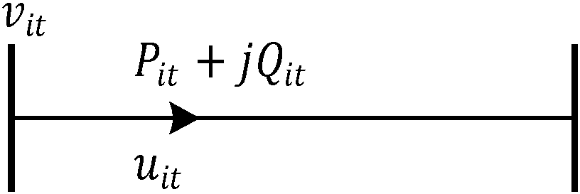
The net active power drawn from the grid at each bus is calculated in (33). The load flow (LF) constraints in the radial network are represented by (34)–(37), with the usual convex relaxation of the equality constraint in (37) adopted from [36], which is reported to be exact when the objective of the problem guarantees the minimization of branch currents, as in the considered model. The line model and the labels of the variables are shown in Figure 3.

(3)

Nodal voltage limits.

$${\left({\mathrm{V}}_{\mathrm{m}\mathrm{i}\mathrm{n}}\right)}^2 \le v_{it} \le {\left({\mathrm{V}}_{\mathrm{m}\mathrm{a}\mathrm{x}}\right)}^2$$

(38)

Constraint (38) bounds the voltage deviation.

(4)

Thermal limits on distribution lines.

$$u_{it} \le {\mathrm{u}}_i^{\mathrm{m}\mathrm{a}\mathrm{x}}, {\mathrm{u}}_i^{\mathrm{m}\mathrm{a}\mathrm{x}}={\mathrm{u}}_{i0}^{\mathrm{m}\mathrm{a}\mathrm{x}}+{\sum }_{l\in {\mathsf{\Theta }}^{\mathrm{l}}}{x}_{il}^{\mathrm{L}}\left({\mathrm{u}}_l^{\mathrm{m}\mathrm{a}\mathrm{x}}-{\mathrm{u}}_{i0}^{\mathrm{m}\mathrm{a}\mathrm{x}}\right)$$

(39)

The thermal limit (39) maintains the current in the transformer and lines below their maximum capacity.

(5)

DG operation constraints.

$${\mathrm{p}}_{i,\mathrm{m}\mathrm{i}\mathrm{n}}^{\mathrm{D}\mathrm{G}} \le p_{it}^{\mathrm{D}\mathrm{G}} \le {\mathrm{p}}_{i,\mathrm{m}\mathrm{a}\mathrm{x}}^{\mathrm{D}\mathrm{G}}$$

(40)

The output of DG units is subject to generation limits (40).

(6)

ESS operation constraints.

$${SoC}_{it}^{\mathrm{E}\mathrm{S}\mathrm{S}} \le \mathrm{M}{\sum }_{o\in {\mathsf{\Theta }}^{\mathrm{E}\mathrm{S}\mathrm{S}}}{x}_{io}^{\mathrm{E}\mathrm{S}\mathrm{S}}$$

(41)

$$\left\{\begin{array}{c}{\mathrm{S}\mathrm{o}\mathrm{C}}_{i,\mathrm{m}\mathrm{a}\mathrm{x}}^{\mathrm{E}\mathrm{S}\mathrm{S}}={\sum }_{o\in {\mathsf{\Theta }}^{\mathrm{E}\mathrm{S}\mathrm{S}}}{\overline{\mathrm{S}\mathrm{o}\mathrm{C}}}_o{x}_{io}^{\mathrm{E}\mathrm{S}\mathrm{S}}, {\mathrm{S}\mathrm{o}\mathrm{C}}_{i,\mathrm{m}\mathrm{i}\mathrm{n}}^{\mathrm{E}\mathrm{S}\mathrm{S}}={\sum }_{o\in {\mathsf{\Theta }}^{\mathrm{E}\mathrm{S}\mathrm{S}}}{\underset{\_}{\mathrm{S}\mathrm{o}\mathrm{C}}}_o{x}_{io}^{\mathrm{E}\mathrm{S}\mathrm{S}}\\ {\mathrm{p}\mathrm{c}}_{i,\mathrm{m}\mathrm{a}\mathrm{x}}^{\mathrm{E}\mathrm{S}\mathrm{S}}={\sum }_{o\in {\mathsf{\Theta }}^{\mathrm{E}\mathrm{S}\mathrm{S}}}\overline{{\mathrm{p}\mathrm{c}}_o}{x}_{io}^{\mathrm{E}\mathrm{S}\mathrm{S}}, {\mathrm{p}\mathrm{d}}_{i,\mathrm{m}\mathrm{a}\mathrm{x}}^{\mathrm{E}\mathrm{S}\mathrm{S}}={\sum }_{o\in {\mathsf{\Theta }}^{\mathrm{E}\mathrm{S}\mathrm{S}}}\overline{{\mathrm{p}\mathrm{d}}_o}{x}_{io}^{\mathrm{E}\mathrm{S}\mathrm{S}}\end{array}\right.$$

(42)

$${\mathrm{S}\mathrm{o}\mathrm{C}}_{i,\mathrm{m}\mathrm{i}\mathrm{n}}^{\mathrm{E}\mathrm{S}\mathrm{S}} \le {SoC}_{it}^{\mathrm{E}\mathrm{S}\mathrm{S}} \le {\mathrm{S}\mathrm{o}\mathrm{C}}_{i,\mathrm{m}\mathrm{a}\mathrm{x}}^{\mathrm{E}\mathrm{S}\mathrm{S}}$$

(43)

$${pc}_{it}^{\mathrm{E}\mathrm{S}\mathrm{S}} \le {\mathrm{p}\mathrm{c}}_{i,\mathrm{m}\mathrm{a}\mathrm{x}}^{\mathrm{E}\mathrm{S}\mathrm{S}}, {pd}_{it}^{\mathrm{E}\mathrm{S}\mathrm{S}}\le {\mathrm{p}\mathrm{d}}_{i,\mathrm{m}\mathrm{a}\mathrm{x}}^{\mathrm{E}\mathrm{S}\mathrm{S}}$$

(44)

$${SoC}_{it}^{\mathrm{E}\mathrm{S}\mathrm{S}}={SoC}_{i,t-1}^{\mathrm{E}\mathrm{S}\mathrm{S}}+{\mathsf{\eta }}_c{pc}_{it}^{\mathrm{E}\mathrm{S}\mathrm{S}}-{\displaystyle \frac{1}{{\mathsf{\eta }}_d}}{pd}_{it}^{\mathrm{E}\mathrm{S}\mathrm{S}}$$

(45)

$${pc}_{it}^{\mathrm{E}\mathrm{S}\mathrm{S}} \le \mathrm{M}{\alpha }_{it}^{\mathrm{E}\mathrm{S}\mathrm{S}}, {pd}_{it}^{\mathrm{E}\mathrm{S}\mathrm{S}} \le \mathrm{M}\left(1-{\alpha }_{it}^{\mathrm{E}\mathrm{S}\mathrm{S}}\right)$$

(46)

$${BDC}_i^{\mathrm{E}\mathrm{S}\mathrm{S}}={\mathrm{B}\mathrm{D}}_i^{\mathrm{E}\mathrm{S}\mathrm{S}}{\sum }_{t\in {\mathsf{\Theta }}^{\mathrm{t}}}\left({pc}_{it}^{\mathrm{E}\mathrm{S}\mathrm{S}}+{pd}_{it}^{\mathrm{E}\mathrm{S}\mathrm{S}}\right)$$

(47)

$${\mathsf{\eta }}_c{\sum }_{t\in {\mathsf{\Theta }}^{\mathrm{t}}}{pc}_{it}^{\mathrm{E}\mathrm{S}\mathrm{S}}={\displaystyle \frac{1}{{\mathsf{\eta }}_d}}{\sum }_{t\in {\mathsf{\Theta }}^{\mathrm{t}}}{pd}_{it}^{\mathrm{E}\mathrm{S}\mathrm{S}}$$

(48)

The operation of the ESSs is modeled in (41)–(48). The $SoC$ in the ESS is subject to its availability in (41). The upper and lower bounds for the $SoC$, as well as the maximum charging and discharging power of the ESS, are defined in (42). The SoC in the ESS is constrained by its capacity limits in (43). The charging and discharging power of the batteries are subject to the output limits in (44). The SoC in the ESS is obtained in (45). The charging or discharging mode of the ESS is determined in (46). The battery degradation cost is presented in (47). Finally, the net energy stored in the ESS over a day is forced to be zero in (48).

With a static design of NC, the utility sets a constant NC fee for all the network buses throughout the day, regardless of the different strain on the network infrastructure. In a dynamic NC design, NC can take different values to better represent the actual operational costs and grid needs. In a planning and operation model for the utility, $n{c}_{it}$ denotes the NC level at bus $\mathrm{i}$ during time interval $\mathrm{t}$. For example, in a 23-bus network, there are 23 × 24 = 552 NC variables for a day with 24 one-hour time intervals.

5. Methodology

The DN planning model that integrates end-user decisions is treated as a one-leader, n-follower SG, where the feasible strategy sets, and their objective functions are provided in (3) and (4), respectively. The utility acts as the leader and the users are treated as the followers. In this game, all the players are satisfied with the final solution, such that no player has an incentive to deviate from the solution of the SG model. Such a solution is referred to as the SE. To find the SE, the game is modeled as bilevel programming problem following the procedure presented in [37], which applies a column-and-constraint-based decomposition and converges to the optimal solution in a finite number of iterations. The adopted reformulation technique converts the original bilevel programming problem into an equivalent single-level problem, as proven in [37,38]. The reformulated problem is further decomposed using BD, which is guaranteed to converge to the global optimal solution when the subproblem is convex [39]. The final reformulated and decomposed problems are presented in (10), (11) and (12).

The bilevel model of the $\mathrm{S}\mathrm{G}1$ is presented in (50)–(57),

$$\mathrm{S}\mathrm{G}1:$$

$$\underset{X^{\mathrm{u}}, Y^{\mathrm{u}}, X^{\mathrm{c}0}, Y^{\mathrm{c}0}}{\min }{F}_u{\left[X^{\mathrm{u}}, Y^{\mathrm{u}}, X^{\mathrm{c}0}, Y^{\mathrm{c}0}\right]}^T$$

(49)

$$\mathrm{s}.\mathrm{t}. {\mathsf{\Psi }}_{\mathrm{u}}{\left[X^{\mathrm{u}}, Y^{\mathrm{u}}, X^{\mathrm{c}0}, Y^{\mathrm{c}0}\right]}^{\mathrm{T}} \le {{\mathsf{\Delta }}_{\mathrm{u}}}^{\mathrm{T}}$$

(50)

$${\mathsf{\Omega }}_{\mathrm{u}}{\left[X^{\mathrm{u}}, Y^{\mathrm{u}}, X^{\mathrm{c}0}, Y^{\mathrm{c}0}\right]}^{\mathrm{T}}={{\mathsf{\Lambda }}_{\mathrm{u}}}^{\mathrm{T}}$$

(51)

$${\mathsf{\Psi }}_{\mathrm{L}\mathrm{F}}\left(X^{\mathrm{u}}, Y^{\mathrm{u}}, X^{\mathrm{c}0}, Y^{\mathrm{c}0}\right) \le 0$$

(52)

$${\mathsf{\Omega }}_{\mathrm{L}\mathrm{F}}\left(X^{\mathrm{u}}, Y^{\mathrm{u}}, X^{\mathrm{c}0}, Y^{\mathrm{c}0}\right)=0$$

(53)

$$\left(X^{\mathrm{c}0}, Y^{\mathrm{c}0}\right)\in \mathit{arg}{\min }_{X^{\mathrm{c}}, Y^{\mathrm{c}}}{F}_{\mathrm{c}}{\left[X^{\mathrm{u}}, Y^{\mathrm{u}}, X^{\mathrm{c}}, Y^{\mathrm{c}}\right]}^{\mathrm{T}}$$

(54)

$$\mathrm{s}.\mathrm{t}. {\mathsf{\Psi }}_{\mathrm{c}}{\left[X^{\mathrm{u}}, Y^{\mathrm{u}}, X^{\mathrm{c}}, Y^{\mathrm{c}}\right]}^{\mathrm{T}} \le {{\mathsf{\Delta }}_{\mathrm{c}}}^{\mathrm{T}}$$

(55)

$${\mathsf{\Omega }}_{\mathrm{c}}{\left[X^{\mathrm{u}}, Y^{\mathrm{u}}, X^{\mathrm{c}}, Y^{\mathrm{c}}\right]}^{\mathrm{T}}={{\mathsf{\Lambda }}_{\mathrm{c}}}^{\mathrm{T}}$$

(56)

where $X^{\mathrm{u}}$, $Y^{\mathrm{u}}$, $X^{\mathrm{c}}$ and $Y^{\mathrm{c}}$ are the integer variables in (28)–(48), continuous variables in (28)–(48), integer variables in (25)–(27), and continuous variables in (25)–(27), respectively. $F_u$ and $F_c$ are the matrix of multipliers of the objective functions described in (29) and (26), respectively. In (50) and (51), all constraints in (32)–(48), except the load flow Equations (33)–(37), are included. The load flow Equations (33)–(37) are represented in (52) and (53). The constraints in (27) are duplicated in (55) and (56). It is worth noting that $F_{\mathrm{u}}$, ${\mathsf{\Psi }}_{\mathrm{u}}$, ${\mathsf{\Omega }}_{\mathrm{u}}$, $F_{\mathrm{c}}$, ${\mathsf{\Psi }}_{\mathrm{c}}$ and ${\mathsf{\Omega }}_{\mathrm{c}}$ are matrices and their corresponding equations are linear, whereas ${\mathsf{\Psi }}_{\mathrm{L}\mathrm{F}}$ and ${\mathsf{\Omega }}_{\mathrm{L}\mathrm{F}}$ are nonlinear functions.

Equation (54) is replaced by the corresponding KKT conditions, as presented in $\mathrm{S}\mathrm{G}2$ formulated in (57)–(69).

$$\mathrm{S}\mathrm{G}2:$$

$$\underset{X^{\mathrm{u}}, Y^{\mathrm{u}}, X^{\mathrm{c}0}, Y^{\mathrm{c}0}, Y^{\mathrm{cz}}, {\mu }^{\mathrm{cz}}, {\vartheta }^{\mathrm{cz}}}{\min }{F}_{\mathrm{u}}{\left[X^{\mathrm{u}}, Y^{\mathrm{u}}, X^{\mathrm{c}0}, Y^{\mathrm{c}0}\right]}^{\mathrm{T}}$$

(57)

$$\mathrm{s}.\mathrm{t}. {\mathsf{\Psi }}_{\mathrm{u}}{\left[X^{\mathrm{u}}, Y^{\mathrm{u}}, X^{\mathrm{c}0}, Y^{\mathrm{c}0}\right]}^{\mathrm{T}} \le {{\mathsf{\Delta }}_{\mathrm{u}}}^{\mathrm{T}}$$

(58)

$${\mathsf{\Omega }}_{\mathrm{u}}{\left[X^{\mathrm{u}}, Y^{\mathrm{u}}, X^{\mathrm{c}0}, Y^{\mathrm{c}0}\right]}^{\mathrm{T}}={{\mathsf{\Lambda }}_{\mathrm{u}}}^{\mathrm{T}}$$

(59)

$${\mathsf{\Psi }}_{\mathrm{L}\mathrm{F}}\left(X^{\mathrm{u}}, Y^{\mathrm{u}}, X^{\mathrm{c}0}, Y^{\mathrm{c}0}\right) \le 0$$

(60)

$${\mathsf{\Omega }}_{\mathrm{L}\mathrm{F}}\left(X^{\mathrm{u}}, Y^{\mathrm{u}}, X^{\mathrm{c}0}, Y^{\mathrm{c}0}\right)=0$$

(61)

$${\mathsf{\Psi }}_{\mathrm{c}}{\left[X^{\mathrm{u}}, Y^{\mathrm{u}}, X^{\mathrm{c}0}, Y^{\mathrm{c}0}\right]}^{\mathrm{T}} \le {{\mathsf{\Delta }}_{\mathrm{c}}}^{\mathrm{T}}$$

(62)

$${\mathsf{\Omega }}_{\mathrm{c}}{\left[X^{\mathrm{u}}, Y^{\mathrm{u}}, X^{\mathrm{c}0}, Y^{\mathrm{c}0}\right]}^{\mathrm{T}}={ {\mathsf{\Lambda }}_{\mathrm{c}}}^{\mathrm{T}}$$

(63)

$$F_{\mathrm{c}}{\left[X^{\mathrm{u}}, Y^{\mathrm{u}}, X^{\mathrm{c}0}, Y^{\mathrm{c}0}\right]}^{\mathrm{T}} \le F_{\mathrm{c}}{\left[X^{\mathrm{u}}, Y^{\mathrm{u}}, X^{\mathrm{c}\mathrm{z}}, Y^{\mathrm{c}\mathrm{z}}\right]}^{\mathrm{T}}$$

(64)

$${\mathsf{\Psi }}_{\mathrm{c}}{\left[X^{\mathrm{u}}, Y^{\mathrm{u}}, X^{\mathrm{c}\mathrm{z}}, Y^{\mathrm{c}\mathrm{z}}\right]}^{\mathrm{T}} \le {{\mathsf{\Delta }}_{\mathrm{c}}}^{\mathrm{T}}$$

(65)

$${\mathsf{\Omega }}_{\mathrm{c}}{\left[X^{\mathrm{u}}, Y^{\mathrm{u}}, X^{\mathrm{c}\mathrm{z}}, Y^{\mathrm{c}\mathrm{z}}\right]}^{\mathrm{T}}={{\mathsf{\Lambda }}_{\mathrm{c}}}^{\mathrm{T}}$$

(66)

$$-{F_{\mathrm{c}\mathrm{y}}}^{\mathrm{T}}+{{\mathsf{\Psi }}_{\mathrm{c}\mathrm{y}}}^{\mathrm{T}}{\mu }^{\mathrm{c}\mathrm{z}}+{{\mathsf{\Omega }}_{\mathrm{c}\mathrm{y}}}^{\mathrm{T}}{\vartheta }^{\mathrm{c}\mathrm{z}}=0$$

(67)

$${\mu }^{\mathrm{c}\mathrm{z}}\perp \left({{\mathsf{\Delta }}_{\mathrm{c}}}^{\mathrm{T}}-{\mathsf{\Psi }}_{\mathrm{c}}{\left[X^{\mathrm{u}}, Y^{\mathrm{u}}, X^{\mathrm{c}\mathrm{z}}, Y^{\mathrm{c}\mathrm{z}}\right]}^{\mathrm{T}}\right)$$

(68)

$${\mu }^{\mathrm{c}\mathrm{z}}\ge 0, X^{\mathrm{c}\mathrm{z}}\in {\mathsf{\Theta }}^{\mathrm{X}}$$

(69)

where $X^{\mathrm{c}0}$ and $Y^{\mathrm{c}0}$ are dummy variables used to duplicate the lower-level variables in the upper-level problem (ULP). Also, $X^{\mathrm{c}\mathrm{z}}$ is a given candidate solution for the integer variables of the lower-level problem, thus becoming a constant parameter for the ULP. Moreover, $Y^{\mathrm{c}\mathrm{z}}$ is introduced to find the optimal solution for the lower-level problem for any given set of $\left(X^{\mathrm{u}},Y^{\mathrm{u}},X^{\mathrm{c}\mathrm{z}}\right)$. The KKT conditions of the lower-level problem are given in (67)–(69). The model $\mathrm{S}\mathrm{G}2$ described in (57)–(69) is the ULP.

Formulation $\mathrm{S}\mathrm{G}2$ in (57)–(69) has a decomposable structure, where (57)–(63) can be treated as the master problem and (64)–(69) as the subproblem. However, due to the nonconvexity of the subproblem, BD cannot be applied directly. This nonconvexity arises from the bilinear constraint (68), which represents a KKT condition. Note that the subproblem contains no integer variables, as the integer variables in the original end-users’ formulation, $X^{\mathrm{c}\mathrm{z}}$, are enumerated and handled iteratively, resulting in a subproblem with only continuous variables. The nonconvexity due to (68) is addressed by relaxing the constraint (64) using the auxiliary variable ${\epsilon }_z$ and reformulating the subproblem, as follows:

$$\mathrm{S}\mathrm{G}3-\mathrm{M}\mathrm{P}:$$

$$\underset{X^{\mathrm{u}}, Y^{\mathrm{u}}, X^{\mathrm{c}0}, Y^{\mathrm{c}0}}{\min }{F}_{\mathrm{u}}{\left[X^{\mathrm{u}}, Y^{\mathrm{u}}, X^{\mathrm{c}0}, Y^{\mathrm{c}0}\right]}^{\mathrm{T}}$$

(70)

s.t. (58)–(63)

(71)

$$0\ge {{\epsilon }_z}^{*}+\mathsf{\Xi }\left({\left[X^{\mathrm{u}}, Y^{\mathrm{u}}\right]}^{\mathrm{T}}-{\left[X^{\mathrm{u}*}, Y^{\mathrm{u}*}\right]}^{\mathrm{T}}\right)$$

(72)

$$\mathrm{S}\mathrm{G}3-\mathrm{S}\mathrm{P}:$$

$$\underset{Y^{\mathrm{cz}}}{\min }{F}_{\mathrm{c}}{\left[X^{\mathrm{u}}, Y^{\mathrm{u}}, X^{\mathrm{c}\mathrm{z}}, Y^{\mathrm{c}\mathrm{z}}\right]}^{\mathrm{T}}+\varrho {\epsilon }_z$$

(73)

s.t. (65)–(66)

(74)

$$X^{\mathrm{u}}=X^{\mathrm{u}*}, Y^{\mathrm{u}}=Y^{\mathrm{u}*}, X^{\mathrm{c}\mathrm{z}}\in {\mathsf{\Theta }}^{\mathrm{X}}, {\epsilon }_z\ge 0$$

(75)

$${\epsilon }_z\ge F_{\mathrm{c}}{\left[X^{\mathrm{u}}, Y^{\mathrm{u}}, X^{\mathrm{c}0}, Y^{\mathrm{c}0}\right]}^{\mathrm{T}}-F_{\mathrm{c}}{\left[X^{\mathrm{u}}, Y^{\mathrm{u}}, X^{\mathrm{c}\mathrm{z}}, Y^{\mathrm{c}\mathrm{z}}\right]}^{\mathrm{T}}$$

(76)

where the original ULP in (57)–(69) is decomposed into a master problem ($\mathrm{S}\mathrm{G}3-\mathrm{M}\mathrm{P}$) in (70)–(72) and an LP subproblem ($\mathrm{S}\mathrm{G}3-\mathrm{S}\mathrm{P}$) in (73)–(76). A cut is added to $\mathrm{S}\mathrm{G}3-\mathrm{M}\mathrm{P}$ at each iteration, as presented in (72). Since the subproblem is an LP formulation, strong duality holds, and the Benders decomposition cuts generated at each iteration are valid, ensuring that the iterative procedure converges to the optimal solution of the decomposed problem.

To calculate $\mathsf{\Xi }$, let $\widehat{\mathsf{\Xi }}$ be the vector of Lagrangian multipliers associated with constraints $X^{\mathrm{u}}=X^{\mathrm{u}*}$ and $Y^{\mathrm{u}}=Y^{\mathrm{u}*}$ in $\mathrm{S}\mathrm{G}3-\mathrm{S}\mathrm{P}$ presented in (73)–(76). The multipliers in $\widehat{\varpi }$ can be interpreted as the impact of variation in $\left[X^{\mathrm{u}}, Y^{\mathrm{u}}\right]$ on the value of the optimal objective function, i.e., $F_{\mathrm{c}}{\left[X^{\mathrm{u}}, Y^{\mathrm{u}}, X^{\mathrm{c}\mathrm{z}}, Y^{\mathrm{c}\mathrm{z}}\right]}^{\mathrm{T}}+\varrho {\epsilon }_z$. We are only interested in their impact on ${\epsilon }_z$ to create the optimality cut (72). If (76) is not binding, then the impacts of $X^{\mathrm{u}}=X^{\mathrm{u}*}$ and $Y^{\mathrm{u}}=Y^{\mathrm{u}*}$ are zero; thus, no cut is added to $\mathrm{S}\mathrm{G}3-\mathrm{M}\mathrm{P}$. If (76) is binding, then $\widehat{\mathsf{\Xi }}=\varrho \mathsf{\Xi }$ for all variables except ${nc}_{itg}$, i.e., the level of NC. Note that those variables have no impact on the optimal solution of $F_{\mathrm{c}}{\left[X^{\mathrm{u}}, Y^{\mathrm{u}}, X^{\mathrm{c}\mathrm{z}}, Y^{\mathrm{c}\mathrm{z}}\right]}^{\mathrm{T}}$, which means that their associated Lagrangian multipliers only refer to their impact on $\varrho {\epsilon }_z$. Let the impact of ${nc}_{itg}$ on $F_{\mathrm{c}}{\left[X^{\mathrm{u}}, Y^{\mathrm{u}}, X^{\mathrm{c}\mathrm{z}}, Y^{\mathrm{c}\mathrm{z}}\right]}^{\mathrm{T}}$ and $F_{\mathrm{c}}{\left[X^{\mathrm{u}}, Y^{\mathrm{u}}, X^{\mathrm{c}0}, Y^{\mathrm{c}0}\right]}^{\mathrm{T}}$ be $x_1$ and $x_2$, respectively. Hence, we can write $\xi =x_1+\varrho \left(x_2-x_1\right)$. In addition, $x_2$ is the Lagrangian multiplier of constraint (83) in the following problem:

$${\min }_{e^{\mathrm{c}0}}{\sum }_{g=1}^{n_g}{2}^{g-1}{e}_{itg}^{\mathrm{c}0}$$

(77)

$$\mathrm{s}.\mathrm{t}. e_{itg}^{\mathrm{c}0}\le {\pi }_{it}^{\mathrm{c}0}$$

(78)

$$e_{itg}^{\mathrm{c}0}\le \mathrm{M}{nc}_{itg}$$

(79)

$$e_{itg}^{\mathrm{c}0}\ge {\pi }_{it}^{\mathrm{c}0}-\mathrm{M}\left(1-{nc}_{itg}\right)$$

(80)

$$e_{itg}^{\mathrm{c}0}\ge 0$$

(81)

$${\pi }_{it}^{\mathrm{c}0}={\pi }_{it}^{\mathrm{c}0*}$$

(82)

$${nc}_{itg}={{nc}_{itg}}^{*}:x_2$$

(83)

Having $x_2$ and $\xi$, $x_1$ can be found using $\xi =x_1+\varrho \left(x_2-x_1\right)$ and the impact of ${nc}_{itg} = {{nc}_{itg}}^{*}$ on ${\epsilon }_z$ is equal to $x_2 - x_1$.

Now, the upper-level problem $\mathrm{S}\mathrm{G}2$ in (57)–(69) is decomposed into a master problem ($\mathrm{M}\mathrm{P}$) and multiple sub-problems ($\mathrm{S}\mathrm{P}$) for any given candidate integer solution of the lower-level problem ($\mathrm{L}\mathrm{L}\mathrm{P}$), as presented in (84)–(85), (86)–(87) and (88), respectively.

$$\mathrm{M}\mathrm{P}:$$

$$\underset{X^{\mathrm{u}},Y^{\mathrm{u}},X^{\mathrm{c}0},Y^{\mathrm{c}0}}{\min }{F}_{\mathrm{u}}{\left[X^{\mathrm{u}}, Y^{\mathrm{u}}, X^{\mathrm{c}0}, Y^{\mathrm{c}0}\right]}^{\mathrm{T}}$$

(84)

s.t. (58)–(63) and (72)

(85)

$$\mathrm{S}\mathrm{P}:$$

$$\underset{Y^{\mathrm{cz}}}{\min }{F}_{\mathrm{c}}{\left[X^{\mathrm{u}}, Y^{\mathrm{u}}, X^{\mathrm{c}\mathrm{z}}, Y^{\mathrm{c}\mathrm{z}}\right]}^{\mathrm{T}}+\varrho {\epsilon }_z$$

(86)

s.t. (65)–(66) and (75)–(76)

(87)

$$\mathrm{L}\mathrm{L}\mathrm{P}:$$

Equations (25)–(27) ∀i ∈ Θ

(88)

Existence of the Stackelberg Equilibrium

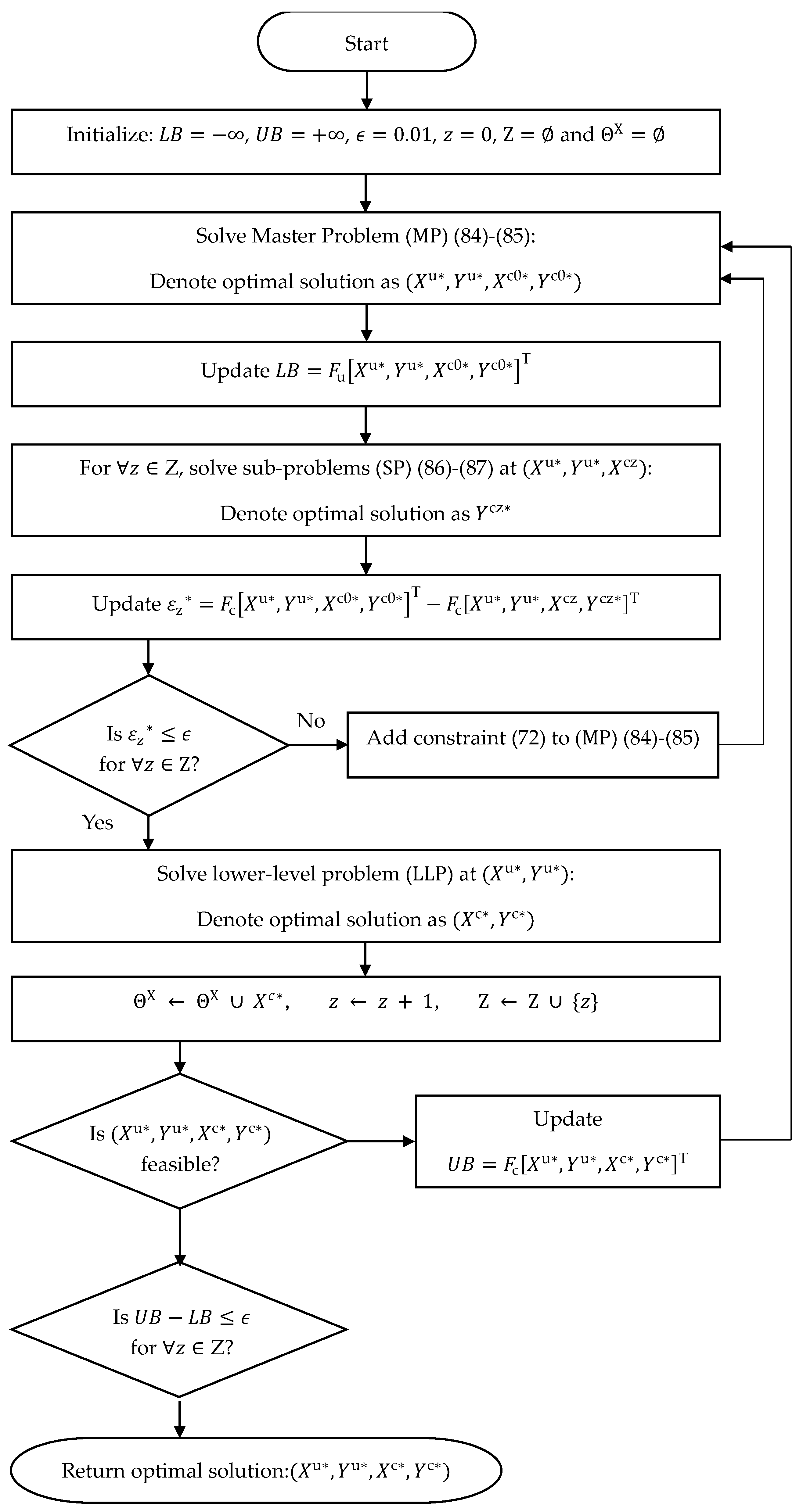
To solve the SPs in (86) and (87), it suffices to solve the $\mathrm{L}\mathrm{L}\mathrm{P}$ in (88) with fixed values for the integer variables. The solution strategy for the ULP and $\mathrm{L}\mathrm{L}\mathrm{P}$s is illustrated in Figure 4. The proposed strategy converts the original bilevel SG model (49)–(56) to an upper-level MISOCP model and a lower-level MILP problem, for which the available commercial solvers like Gurobi can guarantee finding the global optimal solution. The ULP is decomposed into the $\mathrm{M}\mathrm{P}$ (84) and (85) and multiple $\mathrm{S}\mathrm{P}$s (86) and (87). There are two iterative algorithms, i.e., ($\mathrm{M}\mathrm{P},\mathrm{S}\mathrm{P}$) and (ULP, $\mathrm{L}\mathrm{L}\mathrm{P}$). The convergence of the iterative algorithm ($\mathrm{M}\mathrm{P},\mathrm{S}\mathrm{P}$) is guaranteed because $\mathrm{S}\mathrm{P}$ is an LP problem, as reported in [39]. Regarding the convergence of (ULP, $\mathrm{L}\mathrm{L}\mathrm{P}$), if all possible combinations of integer variables in the $\mathrm{L}\mathrm{L}\mathrm{P}$s are known, the problem would be solved in one iteration, as reported in [38]. At any iteration, a new combination of integer variables is added to the model if the algorithm does not converge. As there are a finite number of combinations of integer variables, convergence is guaranteed. Since the reformulated and decomposed problem is equivalent to the original bilevel SG model ($\mathrm{S}\mathrm{G}1$), the proposed solution strategy will converge to the SE. Note that this study avoids full enumeration and instead employs an iterative enumeration technique adopted from [37], making it a practical solution for real-world DNs.

6. Simulations

To examine the proposed model in an LV network, where voltage problems are more likely to occur, a real 23-bus LV DN in Perth, Australia, is selected, which was already adopted as the test case in [40,41,42] (Figure 5). The real-world load data, measured by the meters, as well as the household PV generation profiles extracted from [43] and real-world wholesale market price data obtained from the Australian Energy Market Operator (AEMO) data dashboard [44] are collected and grouped into eight clusters, using a k-means clustering method. The load, PV generation and wholesale price are recorded every hour across one year. The recorded load data are per phase and have been aggregated to three-phase loads, as it is common to consider three-phase balanced systems when planning studies. The probability of each cluster is provided in

Table 1. Probability of clusters.

Cluster No.	1	2	3	4	5	6	7	8
Probability	0.33	0.11	0.02	0.03	0.11	0.16	0.20	0.02

. The simulation parameters are listed in

Table 2. Input parameters to the planning problem.

Parameter	Value
Rated power of candidate PV	3 × 5 kW
Investment cost of candidate PV	3 × $5000
Investment cost of candidate battery	$3000
Rated power of candidate battery	4.5 kW
Rated energy of candidate battery	6 kW
Max-min SoC of candidate battery	5–92%
Charging/discharging efficiency of candidate battery	0.95
Acceptable voltage range	0.90 p.u.–1.05 p.u.
Current capacity of lines	216 A, 251 A and 333 A for cables Mars, Moon, and the new cable
New line’s investment cost	$7500 per km
New transformer’s investment cost	$150 per kVA

. The set of candidate DGs and ESSs are represented in

Table 3. DGs’ characteristics.

DG No.	Rated Power (kW)	Cost Coefficient ($/kWh)	Inv. Cost ($)
1	50	0.375	25,000
2	20	0.500	20,000

and

Table 4. ESSs’ characteristics.

ESS No.	Rated Power (kW)	Rated Energy (kWh)	Inv. Cost ($)	Charge/Discharge Efficiency	Lifetime (Cycles)
1	14	30	10,000	0.95	6000
2	10	20	8500	0.95	6000

. Four cases are studied as follows:

(Case 1) Integrated planning with no NETS (base case).

(Case 2) Integrated planning with NETS and dynamic NC.

(Case 3) Integrated planning with NETS and static NC.

(Case 4) Integrated planning with no investment by end-users.

The total, investment, and operating costs incurred by the utility and end-users are listed in

Table 5. Comparison of results.

Case No.	Costs Incurred to the Utility			Costs Incurred to End-Users			Total Cost ($/yr)
	Total ($/yr)	Inv. ($/yr)	Opr. ($/yr)	Total ($/yr)	Inv. ($/yr)	Opr. ($/yr)
1	−8631	9364	−17,995	197,529	11,096	186,433	188,898
2	−14,600	2263	−16,863	196,511	11,461	185,050	181,911
3	−7655	9364	−17,019	196,553	11,096	185,457	188,898
4	−14,726	7101	−21,827	200,577	0	200,577	185,851

. While end-users’ total cost varies slightly among cases 1–3, the total cost of electrification was reduced by $6987 per year (3.7%) in case 2 compared to cases 1 and 3. This was mainly due to a $7101 saving per year in the utility’s investment cost in case 2 compared to cases 1 and 3. The saving represents the value of the proposed method (case 2) in avoiding unnecessary grid upgrades.

Although cases 1 and 3 resulted in different solutions, the investment plans for the utility and end-users were similar, as was the total cost of electrification. This highlights that a static NC (case 3) will not effectively encourage users to either adopt more DERs or to use them to assist the utility. Some differences in the total cost borne by the utility or users merely arose from the exchange of money between the utility and users. Essentially, the utility’s total cost in case 1 was $976 per year lower than in case 3, while the customers’ total cost in case 1 was $976 per year higher than in case 3.

In case 4, i.e., the conventional approach, no customer investments could take place, but the NET was active, and end-users who already owned DERs could trade energy with others. While the utility’s profit in case 4 is $126 higher than in case 2, it still had to spend an extra $4838 per year to replace the transformer and branch L7, which could have been avoided, as in case 2. Also, the users were $4066 per year better off if they could install DERs. Furthermore, the total cost of electrification increased by 2.1%, from $181,911 per year in case 2 to $185,851 per year in case 4, which reflects the cost of preventing end-users from installing DERs.

The benefit of selling energy to consumers is high enough to compensate for other utility costs, resulting in a negative total cost for the utility (Table 5). Also, the end-users in this LV network are mainly residential, and their consumption is dominant. Therefore, installing one PV unit does not change the fact that they have a much higher daily electricity consumption than generation. That is why they have a positive total cost.

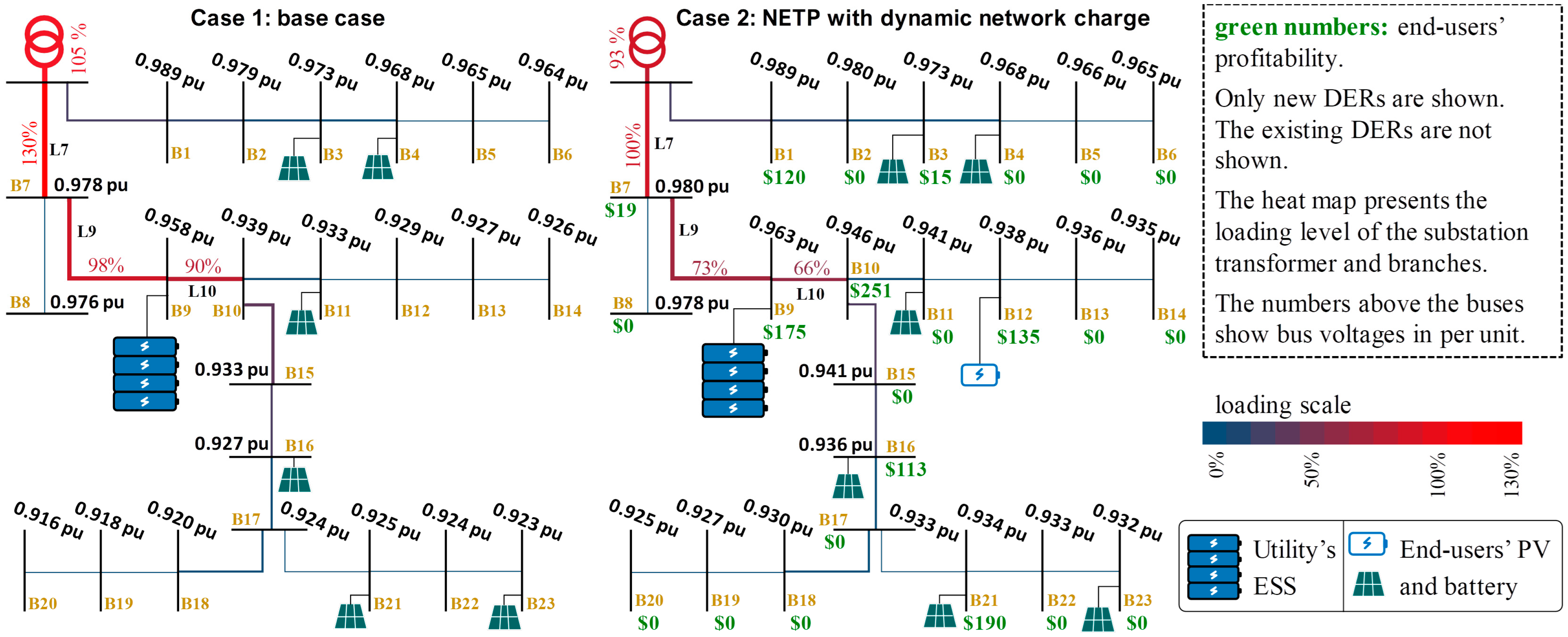
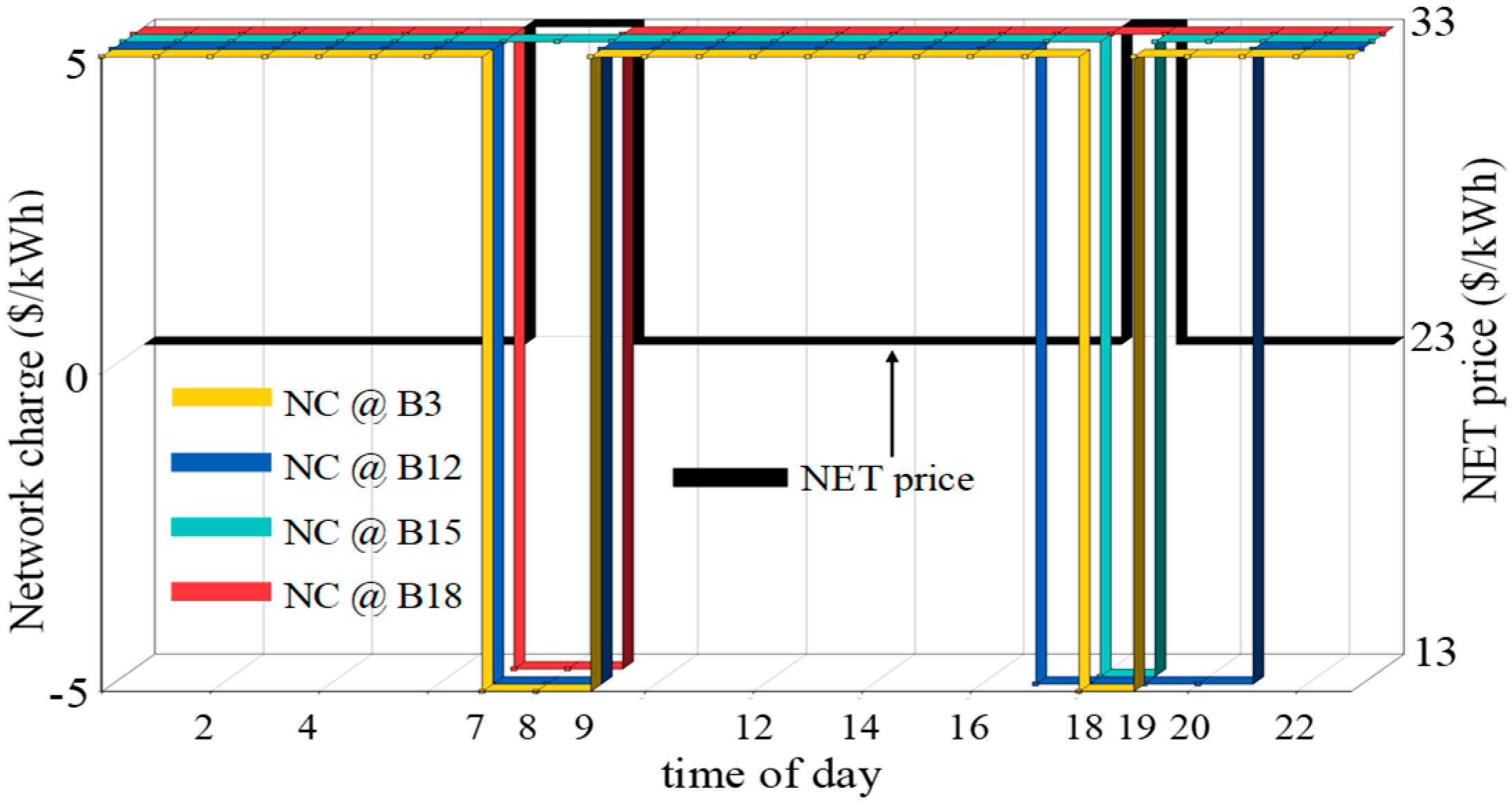
The implementation of the NET and dynamic NC had a pronounced impact on the investment plan of the utility and the end-users (Figure 5). The new battery installed at B12 discharges completely and provides 4.5 kWh of energy during the period 6 P.M.–7 P.M. in cluster 8, of which 4.1 kWh is sold in the NETS, and the remaining 0.4 kWh is self-consumed. The utility offered to pay $5 per kWh to the end-user located at B12 during this time slot for energy trading with others, making it profitable for the end-user to sell the energy stored in the battery in the NETS.

The overloading in the substation transformer and the branch L7 in case 1 is treated in case 2 by utilizing all the available assets in the network, including the DERs on users’ premises. Interestingly, the loading level of the substation transformer and branches L7, L9 and L10 are reduced by 12%, 30%, 25% and 24%, respectively. Analogously, the voltage levels in case 2 are improved when compared to case 1; in particular, all voltages are above 0.92 per unit (p.u.). By changing ${\mathrm{V}}_{\mathrm{m}\mathrm{i}\mathrm{n}}$ to 0.92 p.u., a 50 kW diesel generator (Table 3) was installed at B17 to improve the voltage profile and reduce congestion in the network. This increases the utility’s cost by $840 per year.

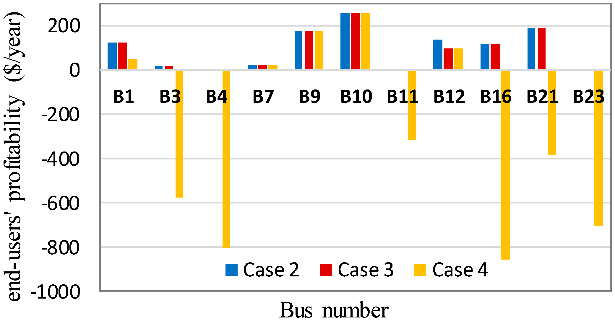
The end-users at B10, B21, B9, B12 and B1 had the highest profitability when comparing case 2 with case 1, in descending order (Figure 6 and Figure 7). No end-user was worse off. Also, the positive profitability at B12 reveals that the revenue earned by the battery at B12 covered the investment cost. The simulations showed that users with more energy available (excess generation from DERs) to sell gained the most from the NETS. Also, the end-users at B3 and B7 had positive profitability of $15 and $19 per year, respectively.

Dynamic NC had a significant impact on energy trades in the NET (Figure 6). Offering negative NC to users at B12 and B15 enabled the NET price to reach $33 per kWh. Given the NC value at B12 during the period from 6 P.M. to 7 P.M. in cluster 8, the end-user at B12 sold the stored energy in his battery for $38 per kWh. Compared to the retail energy price of $28 per kWh, this shows a 36% increase in the value of energy in the NET during that period.

Figure 7 presents the profitability of end-users in cases 2–4 compared to case 1. End-users without changes in their total cost among all cases are not shown. This figure shows that the end-users who acted as sellers in the NETS made the most profit, while those who always acted as buyers saw no profit. This is expected, as the total demand is always greater than the total generation in this network, which drives the cost of buying electricity from the NET (sum of NET price and NC) up to the retail price. In other words, it is profitable for sellers but makes no difference for buyers, which align well with [20]. Moreover, every end-user with a newly installed PV unit in case 1 (Figure 5) incurred higher costs in case 4, due to not investing in PV units when compared to case 1. This applies to end-users at B3, B4, B11, B16, B21 and B23. Also, case 4 is more profitable than case 1 for end-users that had excess generation from existing DERs to sell in the NETS (i.e., the end-users at B1, B7, B9, B10 and B12).

7. Conclusions

The paper aims to provide an improved planning framework that could be exploited by power utilities to achieve a more efficient and affordable development of modern power distribution networks.

The proposed approach includes the effects of the expected optimal decisions by end-users in the utility’s decision-making process. Moreover, the procedure provides an indication of the NC levels that should be applied to end-users participating in neighborhood energy trading schemes. The advantages of the proposed approach are: (1) it enables the utility to rationalize the appropriate use of the network by designing the NC, thus avoiding unnecessary and costly investments; (2) it allows end-users to trade energy and make full use of their DER facilities; and (3) it provides a framework to exploit the flexibilities of end-users to address grid needs. Benders decomposition is adopted, providing a fast and accurate solution algorithm for the proposed planning procedure. This study assumes fixed user preferences; therefore, the results represent an upper bound of achievable benefits. Some aspects need further consideration and improved representation in the model, including all sources of uncertainty, such as uncertainty in end-users’ decision-making, reliability costs, and the effects of adopting smart grid technologies.

References

1. Mohtashami, S.; Pudjianto, D.; Strbac, G. Strategic Distribution Network Planning with Smart Grid Technologies. IEEE Trans. Smart Grid 2017, 8, 2656–2664. [Google Scholar] [CrossRef]
2. Shen, X.; Shahidehpour, M.; Han, Y.; Zhu, S.; Zheng, J. Expansion Planning of Active Distribution Networks with Centralized and Distributed Energy Storage Systems. IEEE Trans. Sustain. Energy 2017, 8, 126–134. [Google Scholar] [CrossRef]
3. Asensio, M.; de Quevedo, P.M.; Munoz-Delgado, G.; Contreras, J. Joint Distribution Network and Renewable Energy Expansion Planning Considering Demand Response and Energy Storage—Part I: Stochastic Programming Model. IEEE Trans. Smart Grid 2018, 9, 655–666. [Google Scholar] [CrossRef]
4. Arefi, A.; Abeygunawardana, A.; Ledwich, G. A New Risk-Managed Planning of Electric Distribution Network Incorporating Customer Engagement and Temporary Solutions. IEEE Trans. Sustain. Energy 2016, 7, 1646–1661. [Google Scholar] [CrossRef]
5. Martins, V.F.; Borges, C.L.T. Active Distribution Network Integrated Planning Incorporating Distributed Generation and Load Response Uncertainties. IEEE Trans. Power Syst. 2011, 26, 2164–2172. [Google Scholar] [CrossRef]
6. Amjady, N.; Attarha, A.; Dehghan, S.; Conejo, A.J. Adaptive Robust Expansion Planning for a Distribution Network with DERs. IEEE Trans. Power Syst. 2018, 33, 1698–1715. [Google Scholar] [CrossRef]
7. Ganguly, S.; Samajpati, D. Distributed Generation Allocation on Radial Distribution Networks Under Uncertainties of Load and Generation Using Genetic Algorithm. IEEE Trans. Sustain. Energy 2015, 6, 688–697. [Google Scholar] [CrossRef]
8. Ehsan, A.; Yang, Q. Coordinated Investment Planning of Distributed Multi-Type Stochastic Generation and Battery Storage in Active Distribution Networks. IEEE Trans. Sustain. Energy 2019, 10, 1813–1822. [Google Scholar] [CrossRef]
9. Zhang, C.; Li, J.; Zhang, Y.-J.A.; Xu, Z. Data-Driven Sizing Planning of Renewable Distributed Generation in Distribution Networks with Optimality Guarantee. IEEE Trans. Sustain. Energy 2020, 11, 2003–2014. [Google Scholar] [CrossRef]
10. Melgar-Dominguez, O.D.; Pourakbari-Kasmaei, M.; Mantovani, J.R.S. Adaptive Robust Short-Term Planning of Electrical Distribution Systems Considering Siting and Sizing of Renewable Energy Based DG Units. IEEE Trans. Sustain. Energy 2019, 10, 158–169. [Google Scholar] [CrossRef]
11. Li, Q.; Ayyanar, R.; Vittal, V. Convex Optimization for DES Planning and Operation in Radial Distribution Systems with High Penetration of Photovoltaic Resources. IEEE Trans. Sustain. Energy 2016, 7, 985–995. [Google Scholar] [CrossRef]
12. Tavares, B.; Soares, F.J. An innovative approach for distribution network reinforcement planning: Using DER flexibility to minimize investment under uncertainty. Electr. Power Syst. Res. 2020, 183, 106272. [Google Scholar] [CrossRef]
13. Canizes, B.; Soares, J.; Lezama, F.; Silva, C.; Vale, Z.; Corchado, J.M. Optimal expansion planning considering storage investment and seasonal effect of demand and renewable generation. Renew. Energy 2019, 138, 937–954. [Google Scholar] [CrossRef]
14. Xiao, X.; Wang, F.; Shahidehpour, M.; Li, Z.; Yan, M. Coordination of Distribution Network Reinforcement and DER Planning in Competitive Market. IEEE Trans. Smart Grid 2020, 12, 2261–2271. [Google Scholar] [CrossRef]
15. Mozaffari, M.; Abyaneh, H.A.; Jooshaki, M.; Moeini-Aghtaie, M. Joint Expansion Planning Studies of EV Parking Lots Placement and Distribution Network. IEEE Trans. Ind. Inform. 2020, 16, 6455–6465. [Google Scholar] [CrossRef]
16. Jooshaki, M.; Farzin, H.; Abbaspour, A.; Fotuhi-Firuzabad, M.; Lehtonen, M. A Model for Stochastic Planning of Distribution Network and Autonomous DG Units. IEEE Trans. Ind. Inform. 2020, 16, 3685–3696. [Google Scholar] [CrossRef]
17. Wang, J.; Hu, Z.; Xie, S. Expansion planning model of multi-energy system with the integration of active distribution network. Appl. Energy 2019, 253, 113517. [Google Scholar] [CrossRef]
18. Li, R.; Wang, W.; Wu, X.; Tang, F.; Chen, Z. Cooperative planning model of renewable energy sources and energy storage units in active distribution systems: A bi-level model and Pareto analysis. Energy 2019, 168, 30–42. [Google Scholar] [CrossRef]
19. Ding, T.; Qu, M.; Huang, C.; Wang, Z.; Du, P.; Shahidehpour, M. Multi-Period Active Distribution Network Planning Using Multi-Stage Stochastic Programming and Nested Decomposition by SDDIP. IEEE Trans. Power Syst. 2021, 36, 2281–2292. [Google Scholar] [CrossRef]
20. Kalathil, D.; Wu, C.; Poolla, K.; Varaiya, P. The Sharing Economy for the Electricity Storage. IEEE Trans. Smart Grid 2019, 10, 556–567. [Google Scholar] [CrossRef]
21. Maharjan, S.; Zhu, Q.; Zhang, Y.; Gjessing, S.; Basar, T. Dependable Demand Response Management in the Smart Grid: A Stackelberg Game Approach. IEEE Trans. Smart Grid 2013, 4, 120–132. [Google Scholar] [CrossRef]
22. Kang, J.; Yu, R.; Huang, X.; Maharjan, S.; Zhang, Y.; Hossain, E. Enabling Localized Peer-to-Peer Electricity Trading Among Plug-in Hybrid Electric Vehicles Using Consortium Blockchains. IEEE Trans. Ind. Inform. 2017, 13, 3154–3164. [Google Scholar] [CrossRef]
23. Pamshetti, V.B.; Singh, S.; Thakur, A.K.; Singh, S.P.; Babu, T.S.; Patnaik, N.; Krishna, G.H. Cooperative Operational Planning Model for Distributed Energy Resources with Soft Open Point in Active Distribution Network. IEEE Trans. Ind. Appl. 2023, 59, 2140–2151. [Google Scholar] [CrossRef]
24. Chen, W.; Hao, P.; Wei, Z.; Chen, L. Study on the optimization allocation method of distributed energy storage in an active distribution network taking into account transmission betweenness and source-network-load synergy. Electr. Power Syst. Res. 2025, 247, 111787. [Google Scholar] [CrossRef]
25. Liao, J.; Lin, J.; Wu, G.; Lai, S. Collaborative Optimization Planning Method for Distribution Network Considering “Hydropower, Photovoltaic, Storage, and Charging”. IEEE Access 2024, 12, 172115–172124. [Google Scholar] [CrossRef]
26. Allahvirdizadeh, Y.; Shayanfar, H.; Moghaddam, M.P. A tri-level approach for coordinated transmission and distribution system expansion planning considering deployment of energy hubs. IET Gener. Transm. Distrib. 2022, 16, 3966–4006. [Google Scholar] [CrossRef]
27. Zhang, Y.; Yang, Y.; Zhang, X.; Pu, W.; Song, H. Planning Strategies for Distributed PV-Storage Using a Distribution Network Based on Load Time Sequence Characteristics Partitioning. Processes 2023, 11, 540. [Google Scholar] [CrossRef]
28. Yang, X.; Zhu, L.; Wang, X.; Zhou, F.; Shi, T.; Jiao, F.; Xu, J. MILP-Based Multistage Co-Planning of Generation–Network–Storage in Rural Distribution Systems. Processes 2025, 13, 3859. [Google Scholar] [CrossRef]
29. Messias, R.; Carvalho, P.M.; Sousa, J. Hybrid distribution network planning to incorporate virtual capacity from distributed flexibility resources. Util. Policy 2025, 93, 101892. [Google Scholar] [CrossRef]
30. Mu, C.; Ding, T.; Huang, Y.; Zhu, S.; Siano, P.; Shahidehpour, M.; Shen, X. Distributed Collaboration Method for Peer-to-Peer Transactions in Reconfigurable Distribution Network. IEEE Trans. Power Syst. 2025, 40, 3029–3042. [Google Scholar] [CrossRef]
31. Oliveira, C.; Simões, M.; Bitencourt, L.; Soares, T.; Matos, M.A. Distributed Network-Constrained P2P Community-Based Market for Distribution Networks. Energies 2023, 16, 1520. [Google Scholar] [CrossRef]
32. Yu, M.; Hong, S.H. A Real-Time Demand-Response Algorithm for Smart Grids: A Stackelberg Game Approach. IEEE Trans. Smart Grid 2015, 7, 879–888. [Google Scholar] [CrossRef]
33. Liu, N.; Yu, X.; Wang, C.; Wang, J. Energy Sharing Management for Microgrids with PV Prosumers: A Stackelberg Game Approach. IEEE Trans. Ind. Inform. 2017, 13, 1088–1098. [Google Scholar] [CrossRef]
34. Chen, J.; Zhu, Q. A Stackelberg Game Approach for Two-Level Distributed Energy Management in Smart Grids. IEEE Trans. Smart Grid 2018, 9, 6554–6565. [Google Scholar] [CrossRef]
35. Maleki Delarestaghi, J. Planning of Power Distribution Networks in Local Energy Communities. Ph.D. Thesis, Murdoch University, Murdoch, Australia, 2021. Available online: https://researchportal.murdoch.edu.au/esploro/outputs/doctoral/Planning-of-power-distribution-networks-in/991005542753507891#file-0 (accessed on 23 January 2021).
36. Farivar, M.; Low, S.H. Branch Flow Model: Relaxations and Convexification—Part I. IEEE Trans. Power Syst. 2013, 28, 2554–2564. [Google Scholar] [CrossRef]
37. Yue, D.; Gao, J.; Zeng, B.; You, F. A projection-based reformulation and decomposition algorithm for global optimization of a class of mixed integer bilevel linear programs. J. Glob. Optim. 2019, 73, 27–57. [Google Scholar] [CrossRef]
38. Yue, D.; You, F. Stackelberg-game-based modeling and optimization for supply chain design and operations: A mixed integer bilevel programming framework. Comput. Chem. Eng. 2017, 102, 81–95. [Google Scholar] [CrossRef]
39. Conejo, A.J.; Castillo, E.; Minguez, R.; Garcia-Bertrand, R. Decomposition Techniques in Mathematical Programming: Engineering and Science Applications; Springer: Berlin/Heidelberg, Germany, 2006. [Google Scholar]
40. Pezeshki, H.; Arefi, A.; Ledwich, G.; Wolfs, P.J. Probabilistic Voltage Management Using OLTC and dSTATCOM in Distribution Networks. IEEE Trans. Power Deliv. 2018, 33, 570–580. [Google Scholar] [CrossRef]
41. Su, X.; Masoum, M.A.S.; Wolfs, P.J. Optimal PV Inverter Reactive Power Control and Real Power Curtailment to Improve Performance of Unbalanced Four-Wire LV Distribution Networks. IEEE Trans. Sustain. Energy 2014, 5, 967–977. [Google Scholar] [CrossRef]
42. Pezeshki, H.; Wolfs, P.J.; Johnson, M. Multi-agent systems for modeling high penetration photovoltaic system impacts in distribution networks. In Proceedings of the 2011 IEEE PES Innovative Smart Grid Technologies, Perth, WA, Australia, 13–16 November 2011; pp. 1–8. [Google Scholar] [CrossRef]
43. Ausgrid. Solar Home Electricity Data. Available online: https://near.csiro.au/assets/42966a8f-bc3c-4bde-91d6-91bc5826aa21 (accessed on 23 January 2021).
44. AEMO. Available online: http://data.wa.aemo.com.au/#balancing-summary (accessed on 23 January 2021).
Figure 1. Illustration of the proposed neighborhood energy trading scheme.
Energies 19 01662 g001
Figure 2. Bilevel Stackelberg game model of the distribution network planning.
Energies 19 01662 g002
Figure 3. Illustration of load flow equations.
Energies 19 01662 g003
Figure 4. Solution strategy.
Energies 19 01662 g004
Figure 5. Loading level in branches in a typical day of cluster 8 from 6 P.M. to 7 P.M.
Energies 19 01662 g005
Figure 6. Network charge and the price of electricity in the NETS in cluster 8.
Energies 19 01662 g006
Figure 7. Profitability of end-users compared to case 1 (base case).
Energies 19 01662 g007